HAL Id: hal-02005386
https://hal.archives-ouvertes.fr/hal-02005386
Submitted on 4 Feb 2019
HAL is a multi-disciplinary open access
archive for the deposit and dissemination of
sci-entific research documents, whether they are
pub-lished or not. The documents may come from
teaching and research institutions in France or
abroad, or from public or private research centers.
L’archive ouverte pluridisciplinaire HAL, est
destinée au dépôt et à la diffusion de documents
scientifiques de niveau recherche, publiés ou non,
émanant des établissements d’enseignement et de
recherche français ou étrangers, des laboratoires
publics ou privés.
Joint estimation of tiltmeters drift and volume variation
during reservoir monitoring
Severine Furst, J. Chery, Bijan Mohammadi, M. Peyret
To cite this version:
Severine Furst, J. Chery, Bijan Mohammadi, M. Peyret. Joint estimation of tiltmeters drift and volume
variation during reservoir monitoring. Journal of Geodesy, Springer Verlag, 2019,
�10.1007/s00190-019-01231-3�. �hal-02005386�
Joint estimation of tiltmeters drift and volume variation during
reservoir monitoring
S. Furst
1, J. Chéry
1, B. Mohammadi
2, and M. Peyret
11GM, Univ Montpellier, CNRS, Univ Antilles, Montpellier, France
2IMAG, Univ Montpellier, CNRS, Montpellier, France.
Correspondence to: Severine Furst (severine.furst@gm.univ-montp2.fr)
Abstract. Borehole tiltmeters are widely used to continuously record small surface deformation of reservoirs and
volcanoes. Because these instruments display unknown long-term drift, only short-term tilt signal can be used for monitoring purpose. We propose a method to invert long-term time series of tilt data induced by strain variations at depth. The assumption that tiltmeter drift is linear over time is on its own insufficient to remove the drift and uniquely determine the deformation source parameters. To overcome this problem, we first invert the data with no constrain on the drift to obtain one particular solution among all admissible. Then, using the linearity of the forward model, we use the statistical properties of the drift distributions to restore the uniqueness of the solution. We illustrate our approach with four synthetic cases simulating volume changes of a reservoir. We demonstrate the efficiency of our method and show that the accuracy of estimated volume variation dramatically improves if low drift tiltmeters are used.
Keywords: Modeling, Tiltmeters, Long-term drift, Volcano geodesy, Reservoirs monitoring
1 Introduction
The deformation of the Earth’s surface reflects anthropogenic, tectonic and volcanic processes at depth (e.g., fault slip and/or mass transport) transmitted to the surface through the mechanical properties of the crust. To capture this ground deformation different geodetic instruments and techniques can be used. For instance, Global Navigation Satellite System (GNSS), Interferometric synthetic-aperture radar (InSAR) and levelling surveys commonly monitor millimetric motions of the ground. Complementary to these, tiltmeters locally measure the horizontal derivative of the vertical motion (hereafter denoted as tilt measurement) in one or two directions. These sensitive instruments are suitable for recording small deformations (Goulty, 1976; Agnew, 1986) that would be
beyond the resolution limit of other techniques. Unfortunately, these instruments are drifting with time, with drift rate amplitudes depending on instrument type, making these instruments often unusable for revealing slow deformation processes.
Among the different kind of tiltmeters that have been developed (Agnew, 1986), long-base tiltmeters such as water-tube devices are sensitive to the rotation of a horizontal line with respect to the geoid and therefore measure the horizontal derivative of the vertical motion. Instead, vertical tiltmeters (pendulums) detect the rotation of a vertical line, therefore measuring the vertical derivatives of the horizontal component of motion. Near the free surface of the Earth, these two instruments essentially record the same signal. Nevertheless, due to shear deformation at depth, these signals may be different (Harrison, 1976). Vertical tiltmeters are generally installed close to the free surface in boreholes between 10 and 50 m depth (Jahr et al., 2006) which is relatively shallow compared to the depths of the usual strain sources for volcanoes, geological and geothermal reservoirs, which are usually larger than 1000 m. In such a case, a free surface condition can be assumed and the long-base and short-base tiltmeters should measure the same rotation. Water-tube tiltmeters (10-500 m) are intrinsically stable due to the length of the sensor. To minimize subsurface effects, they are usually installed in deep tunnels therefore displaying residual drifts as low as 0. 1 µrad/yr (e.g. Boudin et al., 2008). By contrast, short-base tiltmeters are usually installed in boreholes and display higher drift rates of 1-100 µrad/y (Jahr et al., 2006, Chawah et al., 2015). Despite borehole tiltmeters are deployed as networks in volcanoes and geological reservoirs (e.g. Gambino et al. 2014), their potential is far from being fully exploited partly because such tiltmeters are drifting in a completely unconstrained way, intrinsically to each instrument. In addition to drift, tiltmeters also display a time dependent noise that can be of various nature, such as environmental (e.g. Goulty, 1976; Gambino et al., 2014) or instrumental (Wu et al., 2015). The environmental noise is mostly induced by hydraulic loading, temperature effect or pressure gradient. These unwanted signals can be lowered when tiltmeters are installed in deep boreholes, to attenuate the amplitude of the noise.
Although the resolution of borehole tiltmeters is as high as 1-5 nrad, tilt data are generally considered only during a short period of time due to the long-term drift and the noise. Indeed, to monitor long-term reservoir extraction or magmatic chamber inflation/deflation, tilt time series with low drift and signal-to-noise ratio are essential (Kohl & Levine, 1993; Wyatt et al., 1982). Previous studies (Ishii et al., 2001; Jahr et al., 2006) applied linear regression in tilt time series to remove the effect of linear trend that can be attributed undiscriminatingly to the sum of instrumental drift and physical processes. In this study, we propose to automatically separate the instrumental drift from the source signal through the solution of an inverse problem. To overcome the non-uniqueness of the solution, we developed a methodology to simultaneously estimate tiltmeters drift as well as strain source parameters from
tilt series. We illustrate our approach with synthetic cases simulating ground deformation induced by a Mogi-type source (Mogi, 1958) whose volume varies over 11 months.
2. Tilt data parametrization
We consider a ground deformation signal recorded by N tiltmeters in both x and y directions directions. For each instrument, the observed tilt 𝑑⃗⃗⃗⃗ (𝑡) is the sum of the signal produced by the source 𝑑𝑜 ⃗⃗⃗⃗ (𝑡), an instrumental drift 𝑠
𝑑𝑑
⃗⃗⃗⃗ (𝑡) and a cumulative noise 𝑐𝑛⃗⃗⃗⃗ (𝑡) as defined by Eq. (1): 𝑑𝑜
⃗⃗⃗⃗ (𝑡) = 𝑑⃗⃗⃗⃗ (𝑡) + 𝑑𝑠 ⃗⃗⃗⃗ (𝑡) + 𝑐𝑛𝑑 ⃗⃗⃗⃗ (𝑡) , (1)
Similarly to gravimeters, the tilt drift can be due to numerous external and internal factors, making its estimation challenging. For spring-based gravimeters, this drift is usually found linear over a few days (Merlet et al., 2008) while an exponential models better the drift associated to supraconducting gravimeters for records longer than 10 years (Van Camp & Francis, 2007). The determination of tiltmeters drift is much more difficult because of the lack of reference instrument or absolute system measurement, but some experiments report linear long term drift over several months of recordings (Sakata & Sato, 1986). Thus, we assume for each instrument that the drift is linear in time such as 𝑑⃗⃗⃗⃗ (𝑡) = 𝑎 ∙ 𝑡 where 𝑎 is a constant drift rate vector (𝑎𝑑 𝑥, 𝑎𝑦) representing the slope of the
drift and 𝑡 is the time elapsed since the beginning of recording. Because the tilt measurement is relative, we assume that the drift is zero at the beginning of observation. The number of unknown drift parameters associated to the problem is therefore 2N.
In the following, we consider that the source strain 𝑑⃗⃗⃗⃗ (𝑡) depends linearly of the source parameter at depth. Strictly 𝑠
speaking, this is obviously not valid in most cases. Nevertheless, such an approximation is considered as reasonable and is widely used in many geophysical domains. For instance, the use of Green functions is widespread for modeling ground deformation induced by dislocation at depth (Okada’s model) or volume changes of a deep reservoir (Mogi or McTigue models). For one source, the time varying deformation captured by the tiltmeters can be written as a product of a known coefficient vector 𝛼 and a continuous time function corresponding to a strain source parameter 𝑝(𝑡) defined by Eq. (2):
𝑑𝑠
⃗⃗⃗⃗ (𝑡) = 𝛼 ∙ 𝑝(𝑡) , (2)
where 𝛼 is called the deformation model parameter and represent the contribution of a unit source parameter to the signal recorded by each tiltmeter. Therefore, larger components in 𝛼 hold for instruments close to the source
indicating a higher sensitivity with respect to the source. Combining Eqs.1 and 2, it becomes obvious that an infinite number of pairs involving 𝑝(𝑡) and N drift rate vectors 𝑎 produce the same signal 𝑑⃗⃗⃗⃗ (𝑡). Therefore, 𝑜
inverting the tilt data yields to a non-unique solution. Instead of converging towards a single global minimum with one set of parameters, the inversion process tends to a family of admissible combinations of parameters, all explaining the data equally well. Eventually, Eq. (3) provides an admissible solution :
𝑑𝑎
⃗⃗⃗⃗ (𝑡) = 𝛼 𝑝𝑎(𝑡) + 𝑎⃗⃗⃗⃗ 𝑡 = 𝛼 𝑝𝑎 ∗(𝑡) + 𝑎⃗⃗⃗⃗ 𝑡 , ∗ (3)
where the subscript a expresses any of all admissible scenarios provided by the optimization, one of them being
the desired scenario denoted by the exponent *. We use the statistical properties of the tilt parameters to recover
the desired scenario, that is the closest admissible solution to the target.
3. Optimization problem 3.1 Global optimization
We discretized the strain source parameter function 𝑝(𝑡) over M time steps, leading to a vector of length M. The total number of unknowns is therefore 2N + M, while the number of observations is 2N ∙ M . We follow a classical scheme of optimization to invert our tilt data to find an admissible set of both 𝑝𝑎 and 𝑎⃗⃗⃗⃗ . The free parameters are 𝑎
set to an admissible initial guess with no other a-priori knowledge. This initial set of parameters provides a first model 𝑑⃗⃗⃗⃗⃗ using the constitutive Eqs. 1 and 2. Then, they are compared to the observations 𝑑𝑚 ⃗⃗⃗⃗ through a functional 𝑜
denoted 𝐽. The stopping criteria is based on a target minimum value for the functional to be reached within given maximum number of iterations. Global optimization is necessary since we have no information on the convexity of the cost function and several local minima may be present.We apply a multi-criteria global optimization algorithm (Ivorra et al., 2013) which aims at improving the initial condition for classical gradient-based methods (Mohammadi & Pironneau, 2009).
To build the global functional, we first compare for the N tiltmeters the model prediction 𝑑⃗⃗⃗⃗⃗ to the observations 𝑚
𝑑𝑜
⃗⃗⃗⃗ at a given time 𝑡𝑖 . We use a weighted Euclidian norm as defined by Eq. (4):
𝐹𝑖= 𝐷⃗⃗⃗ 𝑖 𝑡
Σ𝑖−1𝐷⃗⃗⃗ , 𝑖 (4)
where Σ𝑖 is the covariance error matrix of each measurement and 𝐷⃗⃗⃗ = 𝑑𝑖 ⃗⃗⃗⃗ (𝑡𝑜 𝑖) − 𝑑⃗⃗⃗⃗⃗ (𝑡𝑚 𝑖). In order to construct a
𝑡𝑖 and 𝑡𝑖+1. Therefore, the global functional gathering all observations and the corresponding models can be written as Eq. (5): 𝐽 = 1 𝑡𝑀+1−𝑡1∑ 1 2 [𝐹𝑖+ 𝐹𝑖+1][𝑡𝑖+1− 𝑡𝑖] 𝑀−1 𝑖=1 , (5)
The optimization is assumed to be successful whenever this functional is lower than the data uncertainties or while reaching the target minimum value, providing one optimal set (among an inifinite number of others) of 𝑝 and 𝑎 fitting at best the measurements.
3.2 The non-uniqueness problem
At the end of the optimization, we obtain one set of admissible parameters 𝑝𝑎 and 𝑎⃗⃗⃗⃗ that predicts tilt 𝑎
measurements 𝑑⃗⃗⃗⃗ close to our observations 𝑑𝑎 ⃗⃗⃗⃗ . The residual tilt is defined by the difference between the 𝑜
admissible dataset and the observations over the M time steps:
𝑅𝑀𝑆𝑡𝑖𝑙𝑡 = ( ∑𝑀𝑖=1‖𝐷⃗⃗ 𝑖‖2
𝑀 )
1/2
, (6)
This residual can be due to the noise 𝑐𝑛⃗⃗⃗⃗ embedded in the observations but also to some lack of convergence of the minimization process. Due to non-uniqueness, this admissible set of parameters provides a strain source history and a set of drift rates that can greatly differ from the target solution. Starting from the admissible solution (𝑝𝑎 ;
𝑎𝑎
⃗⃗⃗⃗ ) and Eq. 3, the desired solution ( 𝑝∗; 𝑎⃗⃗⃗⃗ ) must satisfy: ∗
𝑎∗
⃗⃗⃗⃗ = 𝑎⃗⃗⃗⃗ − 𝑅 𝛼 , 𝑎 (7a)
𝑝∗= 𝑝
𝑎+ 𝑅∗ 𝑡 , (7b)
where 𝑅 = 𝑝∗−𝑝𝑎
𝑡 is a correction coefficient to be estimated. When varying 𝑅, we get admissible distributions of
𝑎 and 𝑝 . Having no indication on the strain source history 𝑝(𝑡) , we cannot use Eq. 7b to infer a suitable value for 𝑅. By constrast, Eq. 7a contains a-priori information concerning the source model (N components of 𝛼 ) and the drift parameters (N values of 𝑎 ). Because 𝛼 and 𝑎 datasets represent respectively the source effect (dependent to the instrument position with respect to source position) and the instrument properties, they must be statistically independent. Therefore, the value of 𝑅 in Eq. 7b must be chosen to provide a desired solution 𝑎⃗⃗⃗⃗ displaying a lack ∗
𝑅 = 𝑐𝑜𝑣(𝑎⃗⃗⃗⃗⃗ ,𝛼𝑎⃗⃗ )
𝑣𝑎𝑟(𝛼⃗⃗ ) , (8)
meaning that 𝑅 is the coefficient of the linear regression adusting 𝑎⃗⃗⃗⃗ as a function of 𝛼 . Using an example of the 𝑎
time inflation of a buried volumetric source at depth, we show how our methodology leads to recover both the actual drift rates and volumetric source history.
4. Application to reservoir modeling 4.1 Forward model
The above optimization problem requires a linear relation between the source parameters and the observation. Therefore, this class of problem covers numerous elastic solutions (either analytical or numerical) used for reservoir modeling (Segall, 2010). Among them, the so-called Mogi model is the simplest and probably the most widely used analytical solution for a pressurized point source in a homogeneous elastic half-space (Mogi, 1958). The Mogi source is defined by its radius 𝑅, centered at a depth 𝑧𝑠 beneath the free surface at 𝑧 = 0, 𝑧 being
counted positive upwards. A uniform internal pressure 𝑃 is applied to the boundary of the spherical source. The volumetric change associated with the deformation is given by ∆𝑉 =𝜋
𝜇 𝑃𝑅
3 with 𝜇 being the shear modulus. The
system is described by four variables, including the cartesian coordinates of the point source 𝑥⃗⃗⃗ = (𝑥𝑠 𝑠, 𝑦𝑠, 𝑧𝑠) and
the volumetric change (∆𝑉) that plays the role of the parameter 𝑝 in the optimization problem (section 3 above). The Mogi model predicts 3-D surface deformation 𝑢⃗ = (𝑢𝑥, 𝑢𝑦, 𝑢𝑧) at a given observation point 𝑥 = (𝑥, 𝑦, 0). The
ground tilt vector is given by the horizontal derivatives of the vertical displacement 𝑢𝑧= (𝑥, 𝑦). The tilt 𝑑⃗⃗⃗⃗ is 𝑠
therefore the slope of 𝑢𝑧, considering that tilt vectors are pointing in direction of decreasing vertical displacements.
Therefore, 𝑑⃗⃗⃗⃗ = −∇𝑈⃗⃗ 𝑠 𝑧 (𝑈⃗⃗ 𝑧 being the vector made of the uz of all the tiltmeters at the time considered) and the tilt
vector associated to a source is expressed by the following expressions:
𝑑 𝑠= 𝛼 ∆𝑉 , (9a)
𝛼 =3(1−𝜈)
𝜋
−𝑧𝑠 ∙ 𝑟
(𝑧𝑠2+𝑟2)3/2 𝑛⃗ , (9b)
where 𝜈 is the Poisson ratio (chosen to be 0.25), 𝑟 the horizontal distance √(𝑥𝑠− 𝑥)2+ (𝑦𝑠− 𝑦)2 between the
source point and the observation point and 𝑛⃗ the unit vector pointing from the source to the observation point. Even if all four variables (𝑥𝑠, 𝑦𝑠, 𝑧𝑠, ∆𝑉) can be considered as optimization parameters, we choose to fix the position
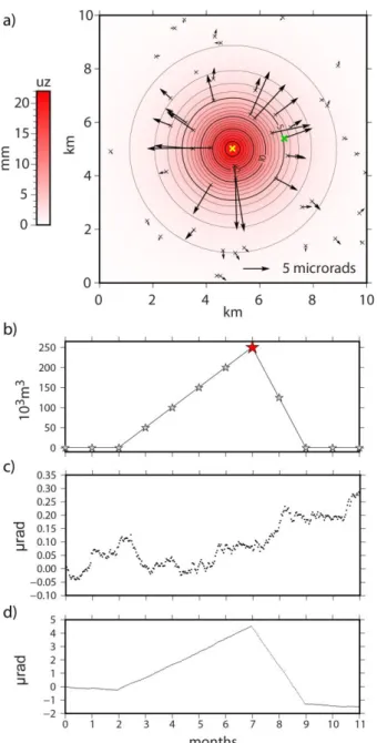
Fig. 1 Synthetic tilt produced by volumetric changes of a spherical source with an added drift of 2.4 µrad/yr and a Brownian noise, during 11 months of the experiment. a) Screenshot of the vertical displacement 𝑢𝑧 (color scale) and tilt signal (black
arrows) induced by a volumetric variation at 𝑡=7 (∆𝑉 = 250 000 m3, red star on b) of a spherical source (yellow cross). b)
Evolution of the targeted volumetric changes over one year c) Typical random walk noise associated to the tilt over 11 months d) Synthetic tilt signal with drift and noise in x-direction for one tiltmeter (green cross on Fig. 1a)
4.2 Synthetic data
In addition to the tilt component induced by the source (Eq. 9a-b), we add to the synthetic signal some random tiltmeter drift and tiltmeter noise to generate 11 months of observations. We present hereafter the results of four different synthetic configurations involving different levels of drift and noise. Each tiltmeter is assumed to have a randomly chosen drift rate for both components using a uniform probability density function. In order to choose the range of probability for drift rates, we use values of available instruments: commercial borehole tiltmeters from Halliburton display a drift of 20-60 µrad/yr (Eric Davis, Pinnacle, personnal communication). According to this information, we use a distribution bounded by ±48 µrad/yr. Chawah et al. (2015) presented the prototype of a low drifting borehole tiltmeter displaying an apparent drift of 0.25 µrad over 2 months (±2.4 µrad/yr) and we use this value to define low drift distribution. Using these two values of drift rates, we aim at studying the behaviour of the optimization scheme to retrieve the instrumental and source parameters. Besides drift, we either consider no noise in the data (Cases 1a and 2a, see table 1) or, to be more realistic, we introduce Brownian noise in tilt data (Cases 1b and 2b). We assign a standard deviation of the short term tilt measurements of 𝜎𝑠ℎ𝑜𝑟𝑡= 5 nrads and assume
that a Brownian noise is leading to a maximum standard deviation 𝜎𝑚𝑎𝑥 at the end of the experiment. Given the
lack of knowledge about noise for the borehole tiltmeters cited above, we arbitrarily set the maximum standard deviation to 180 nrads after one year of experiment. The tilt covariance matrix is therefore built using the maximum standard deviation for both components of each tiltmeter (Kasdin, 1995):
𝜎 = 𝜎𝑠ℎ𝑜𝑟𝑡𝑇𝐴/4 , (10)
where 𝑇 is the number of iterations for each data sample required to reach 𝜎𝑚𝑎𝑥 after 11 months and 𝐴 is the type
of noise (i.e. 𝐴 = 0 for White noise and 𝐴 = 2 for Brownian noise). We estimate 𝑇 to 1440 using Eq. (10) for the specified values of 𝜎𝑠ℎ𝑜𝑟𝑡 and 𝜎𝑚𝑎𝑥. The deformation is produced by a spherical source embedded in an elastic
medium at 1500 m deep and centered in a 10x10 km observation domain. The induced deformation is recorded by 50 tiltmeters randomly distributed (Fig. 1a). Synthetic data are monthly down-sampled to decrease the time size of the problem (M=12), corresponding to monthly time-intervals volume variations (Fig. 1b). The volume change is set to zero during the first 2 months, then increases linearly to 250 000 m3 the next 5 months and finally goes
back to zero after 2 months. The vertical deformation induced by the volume variation of the source is therefore maximum at 𝑡 = 7 months. The corresponding synthetic ground deformation signal at this time is shown for case 1b (low drift instrument and noise of 180 nrad, Fig. 1c). An example of daily time series for x-component of the tilt is shown Fig. 1d for the instrument marked with a green cross on Fig. 1a.
4.3 Results
The configurations and results of the four experiments previously described are summarized in Table 1. After the optimization process, we converge towards an admissible solution with a set of parameters, ∆𝑉𝑎 and 𝑎⃗⃗⃗⃗ giving the 𝑎
lowest residual between synthetic and modelled data, as provided by the RMS value that integrates time series over the whole time period. Table 1 shows a coherent relation between instrumental properties (drift and level of noise) and 𝑅𝑀𝑆𝑡𝑖𝑙𝑡. Indeed, the tilt residual only increases when adding noise to the data (cases 1b and 2b) but not
when the level of drift increases (cases 2a and 2b). The standard deviation associated to the drift values from the optimization (𝑆𝐷𝑜) is significantly higher than the target one (𝑆𝐷𝑡) for cases 1a and b while for cases 2a and b, the
standard deviations are scarcely different. This latter result is due to the initial large value of 𝑆𝐷𝑡. This standard
deviation is directly linked to the uniform distribution chosen to create drift associated to the synthetic tilt data. The inversion process provides a fairly homogeneous tilt residual over time for the whole set of tiltmeters (Fig. 2a). Also, the spatial distribution of the residual values between synthetic and modelled tilt vectors shows a lack of spatial trend for both amplitude and azimuth (Fig. 2b).
Test 1a 1b 2a 2b Configuration Drift (µrad/yr) ±2.4 ±2.4 ±48 ±48 𝑆𝐷𝑡 (µrad/yr) 1.92 1.92 38.61 38.61 Noise (µrad/yr) 0 0.18 0 0.18 Optimization 𝑅𝑀𝑆𝑡𝑖𝑙𝑡 (nrad) 0.59 46.7 3.05 48.2 𝑆𝐷𝑜 (µrad/yr) 9.40 5.60 38.75 38.58
Flow rate trend 𝑉0̇
(103 m3/yr) 2.14 2.03 -181 -182
𝑆𝐷𝑟 (µrad/yr) 1.92 1.94 38.37 38.41
Flow rate uncertainty
𝛿𝑉̇ (103 m3/yr) 14.1 14.2 280 281
Volume resolution 𝛿𝑉 (m3) 6 490 32 506
Table 1 Configurations and results of the combination of global optimization and flow correction for four synthetic cases
(1a-b and 2a-(1a-b). The standard deviation associated to drift rate 𝑆𝐷𝑡 is given for the synthetic values of drift for cases 1 and 2. The
𝑅𝑀𝑆𝑡𝑖𝑙𝑡 describes the mean residual in tilt measurements for all instruments over time. After the inversion, the standard
deviation 𝑆𝐷𝑜associated tothe admissible values of drift rate is calculated for each case. The flow rate trend 𝑉0̇ represents the
is estimated after the flow correction. The flow rate uncertainty 𝛿𝑉̇ and the volume resolution 𝛿𝑉 are provided according Eqs. (11a-b)
Fig. 2 Residual tilt provided by optimization for case 1b. a) Time evolution of the norm of the residual tilt vectors for all
instruments. Red crosses correspond to residual shown in b. b) Tilt residual pattern at t=7 month (black arrows) superimposed to the uplift model (solid isovalues). The position of the spherical source is represented by a yellow cross.
This admissible optimal solution is only one particular solution of the family associated to Eq. 3. Because no constrain is applied at this stage on the relation between 𝛼 (which expresses the dependency of ground measurements on their relative spatial distribution with respect to source location) and drift parameters 𝑎⃗⃗⃗⃗ , a clear 𝑎
correlation pattern occurs between these two quantities (Fig. 3). At the end of the inversion process, this correlation results in a volume variation history reflecting part of the instrumental drift (green dashed line in Fig. 4a). In order to cancel this trend which is caused by the non-uniqueness of the inverse problem, we enforce the lack of correlation between the deformation model parameters 𝛼 and the desired drift parameters 𝑎⃗⃗⃗⃗ by inserting the result ∗
of Eq. (8) in Eq. (7a). As a result, the components of 𝑎⃗⃗⃗⃗ display a variance similar to the one associated to the ∗
target drift coefficients (Fig. 3). In addition, there is an excellent agreement between the desired and target drift values with a residual value of 0.04 µrad/yr for case 1a (Figure 3a), 0.19 µrad/yr for case 1b (Figure 3b) and 4.19
µrad/yr for cases 2a and b (Figure 3c-d). Because this value is slightly smaller than the trend of the synthetic Brownian noise for cases 1a and b (that is in average equal to 0.2 µrad/yr, see Eq. (10) and Fig. 1c), we can conclude that the optimization process retrieves the sum of both deterministic and stochastic linear trends. Once the correction factor 𝑅 is determined, it can be used in Eq. (7b) to obtain the desired volume change ∆𝑉∗. However,
for cases 2a and b, the linear trend introduced by the instrumental drift is largely greater than the linear trend of the synthetic Brownian noise resulting in a lower precision of drift determination. In such configuration, we do not fully retrieve the linear trend of the instrumental drift due to the higher variance associated to the target drift values. For cases 1a and b, sets of drift values obtained after the flow correction have standard deviation (𝑆𝐷𝑟)
markedly equal to the target variance, while for case 2a and b, they slightly differ but remain closed to the expected standard deviation.
Fig. 3 Relation between all components (x-y) of drift rate 𝑎⃗⃗⃗⃗ and model coefficients 𝛼 for all 4 cases of Table 1: a) case 1a, b) 𝑎
case 1b, c) case 2a and d) case 2b. Note the change in vertical scale between a-b and c-d. Black dots refer to the components of 𝑎⃗⃗⃗⃗ that display a clear correlation with 𝛼 components. After a linear correction using the value of 𝑅 provided by Eq. 8, the 𝑎
components of 𝑎⃗⃗⃗⃗ are decorrelated with 𝛼 components. Target coefficients (blue crosses) are retrieved with a precision of 0.04 ∗
µrad/yr fo case 1a, 0.19 µrad/yr.for 1b and 4.19 µrad/yr for cases 2a and b
Because the target volume change after 11 months is zero, the flow trend rate 𝑉0̇ between initial and final values
of ∆𝑉∗ should be zero. Therefore, the modelled value of 𝑉
0̇ in Table 1 provides some insight about the precision
of instrumental drift determination. Unsurprisingly, low drift tiltmeters retrieve precisely the final target volume (Table 1 and Fig. 4a). Similar values of 𝑉0̇ provided by experiments 1a and b (respectively 2a and b) are due to
identical set of the drift coefficients used for these experiments. Beyond these particular solutions, one needs to provide a statistical bound of the solution uncertainty. Two kinds of estimates are needed (1) the volumetric flow rate resolution 𝛿𝑉̇ (i.e. the accuracy of the linear component of the solution along time) (2) the instantaneous volume resolution 𝛿𝑉. The former quantity is associated to the Eq. 7a and to the precision of determination of 𝑅. The latter term 𝛿𝑉is linked to Eq. 9a and to the precision of the determination of 𝑑⃗⃗⃗⃗ that depends in turn from 𝑠
𝑅𝑀𝑆𝑡𝑖𝑙𝑡. Because of the linear character of these equations, uncertainties on 𝛿𝑉̇ and 𝛿𝑉 associated respectively to
𝑅 and ∆𝑉 are given by the following relations:
𝛿𝑉̇ = 𝑅𝑀𝑆𝑎∗⁄(𝛼𝑚𝑎𝑥− 𝛼𝑚𝑖𝑛) , (11a)
𝛿𝑉 = 𝑅𝑀𝑆𝑡𝑖𝑙𝑡⁄(𝛼𝑚𝑎𝑥− 𝛼𝑚𝑖𝑛) , (11b)
where 𝑅𝑀𝑆𝑎∗ is the residual drift rate computed over all components of 𝑎⃗⃗⃗⃗ , 𝛼∗ 𝑚𝑖𝑛 and 𝛼𝑚𝑎𝑥 being the minimum
and maximum values over all components of 𝛼 . The computation of these values in Table 1 indicates that the target volume solution is adequately covered by this a-posteriori uncertainty computation of 𝛿𝑅. Finally, we check by removing the trend associated to targeted and modelled evolutions that the residual volume of the solution over time is bounded by a-posteriori uncertainty 𝛿𝑉, that is of 490 m3 for case 1b (Fig. 4b).
Fig. 4 Evolution of volume variation ∆𝑉 along time for case 1b a) comparison of target volume variation (grey dotted line), modeled volume variation before and after flow correction (green dashed and black solid line), upper and lower modeled volume variation at 2- uncertainties (blue and red dashed lines); b) residual volume equal to the difference between target and modeled volume with the linear trend removed for both solutions
5. Discussion
This two-step optimization approach allows for estimating the strain source change in a reservoir monitored by subsurface tiltmeters displaying a compound of linear drift but also coloured noise. First, the resolution of the inverse problem with no constrain imposed on the drift rate leads to a family of solutions displaying an even
adjustment to the data. The quality of the adjustment is directly linked to the amount of non-linear noise generated (or recorded) by the tiltmeters and does not involve the drift rate. Afterwards, the uniqueness of the solution (volume change and drift rate) is enforced by minimizing the correlation between deformation model parameters 𝛼 (that represents the sensitivity of the tiltmeters to volumetric change at depth) and drift parameters 𝑎 (that should be independent from source parameters). For this second step, the precision of volumetric change retrieval is directly linked to the average magnitude of drift. For the amount of deformation considered here (a maximum tilt of 15 µrad) over a 11-months duration, low drift tiltmeters (2.4 µrad/yr) allow for precise recovery of the trend of the volumetric solution with an uncertainty rate of 14 000 m3/yr for a depth source of 1500 m. By contrast, the
target solution is poorly retrieved if moderate drift tiltmeters are considered. This experiment shows the interest for installing low drifting instruments if small amplitude signals are recorded and long term deformation is sought. On the contrary, a signal significantly larger than the drift signal (e.g. for large volcanic events) will be detected by moderately drifting tiltmeters. We also show that the instantaneous volume uncertainty is linked to the amplitude of Brownian noise associated to the tiltmeters but does not depend on average drift rate amplitude. Therefore, our approach provides a relation between the quality of the tiltmeters (in term of linear drift and noise) and the precision of strain source retrieval for a given network configuration. As far as long-term monitoring is concerned, the value of the short-term standard deviation of the tiltmeter (𝜎𝑠ℎ𝑜𝑟𝑡 in Eq. 10) presents little interest
and must be completed by a quantification about the linear drift rate of the sensor as well as the magnitude of its time-dependent noise.
To our knowledge, no method was previously available to mathematically separate tiltmeters drift from the surface deformation associated to a deep strain source over a monitoring time ranging from months to years. We overcome two difficulties: (1) the relatively large number of free parameters associated to both tiltmeters drift rates and a long strain source history and (2) the lack of a-priori knowledge on drift rates parameters distribution. At this stage, we found that splitting the minimisation step in the inversion problem and the retrieval of the drift parameters enforcing uniqueness makes the problem easy to adapt to different optimization strategies. We noticed however that this two-step method could be replaced by a global formulation. Indeed, removing the correlation between source and drift parameters inside the minimization algorithm can also be achieved by looking for drift parameters having the lowest variance. This multi-criteria problem can be solved introducing, for instance, a weighted functional linear combination of the model-data misfit and the drift parameters variance.
6. Conclusion
In the study, we present a methodology to automatically determine the instrumental drift component of tilt data in order to address the challenge of long-term reservoir monitoring. The following generic key features can be retained:
1. The approach is usable for any forward model involving a linear relation between source parameter (typically volume change) and surface deformation (tilt or strain). Therefore, all small strain elastic formulations involving non-spherical sources (Segall, 2010), opening dislocations (Okada, 1992), or even inhomogeneous distributions of the medium properties (Masterlark et al., 2016) are suitable.
2. Our methodology relies on the assumption of the independence between source parameters and drift parameters. The enforcement of this statistical property provides a way for determining confidence intervals of parameters. This first study suggests that only low drift tiltmeters (ie, lower than a few µrad/yr) are useful for long term geodetic monitoring without additional geodetic measurements like GNSS or InSAR.
3. Instrumental drift and noise can be extracted from the residual signal of a network of tiltmeters. Although we have chosen a low level of noise compared to instrumental drift, this study demonstrates that tilt residual critically depends on the non-linear instrumental behaviour. In addition, the analysis of tilt network residual using approaches developed for GNSS time analysis (Williams, 2003) may bring insight on long-term correlated noise of borehole tiltmeters that is poorly known so far.
4. The methodology could be extended to account for other geodetic measurements like GNSS times series, InSAR and leveling in order to perform a model-data fusion to characterize deep reservoir deformation (e.g. Xu et al., 2009; Wang et al., 2002). In this case, a multi-criteria functional would combine all geodetic measurements with their relative weights and error covariance as well as an estimation of the correlation between drift and source parameters.
Our inverse methodology combined with the low drifting tiltmeters should pave the way for long-term tilt monitoring of concentrated or distributed sources of strain at depth, notably for geothermal areas, oil & gas reservoirs and volcanoes. Widely used in volcanic monitoring (e.g. Anderson et al., 2010; Anderson et al., 2015; Ferro et al., 2011; Gambino et al., 2014; Narváez Medina et al., 2017; Peltier et al., 2009; Poland et al., 2014; Ricco et al., 2018), borehole tiltmeters are commonly used to determine the source location and its associated volume variation. Yet, considering long-term time series of tiltmeters could improve other geodetic studies (e.g. GNSS or InSAR) that are usually conducted to follow the slow strain processes occurring on volcanoes (e.g. gravitational collapse of Mount Etna’s flank, Urlaub et al., 2018). Additionally, tilt networks are valuable to monitor hydraulic fracturing performed to increase permeability of non-conventional reservoir (Astakhov et al.,
2012; Fisher & Warpinski, 2011; Warpinski, 2014; Wright et al., 1998; Wright et al., 1997). In particular, Warpinski (2014) described the current and future uses that tiltmeters network can provide when used in unconventional operating conditions. This includes: 1) mapping fracture’s network (Wright et al., 1998; Wright et al., 1997; Zhou et al., 2015), 2) orthogonal and horizontal fractures identification, 3) refracturation processes and 4) fracture’s network evolution during fracking processes. Because the ground deformation induced by a single frack is so small (tens of nanometers, Astakhov et al., 2012), only tiltmeters and strainmeters can measure it. The exploitation of a reservoir involves several stages of hydraulic fracturation before resource extraction, inducing a long-term evolution of volume variations (up to 2-3 years). Therefore, it is mandatory to extract the instrumental drift from the data to monitor this deformation. Combined to InSAR studies, this would also permit to properly identify volumes that are stimulated and drained. Finally, geodetic studies have highlighted significant surface
deformations for various geothermal reservoirs principally measured by InSAR (e.g. Ali et al., 2016; Eneva et al., 2012; Falorni et al., 2011; Heimlich et al., 2015; Vasco et al., 2002; Vasco et al., 2013) but also using tiltmeters (Vasco et al., 2002a). Modelling experiments of Im et al. (2017) show that observed surface subsidence may largely result from thermal contraction but also from slow slip reactivation. Because of its long-term stability and its low cost, InSAR data are commonly used to monitor geothermal fields. To the contrary, tilt observations provide a dense temporal sampling associated to a high sensitivity. A key issue is therefore to remove instrumental drift from long term tilt series to overcome the issue of long term stability of tiltmeter. Therefore, coupling InSAR and tilt data in the inversion would lead to a reservoir evolution including small transient events only detectable by high resolution tiltmeters.
Acknowledgments
The PhD of S. Furst is supported by the Total Company and the LabEx NUMEV project (n° ANR-10-LABX-20) funded by the “Investissements d'Avenir” French Government program, managed by the French National Research Agency(ANR).
References
Agnew, D. C. Strainmeters and tiltmeters. Reviews of Geophysics, 24(3), 579-624, 1986.
Ali, S. T., Akerley, J., Baluyut, E. C., Cardiff, M., Davatzes, N. C., Feigl, K. L., … Zemach, E. (2016). Time-series analysis of surface deformation at Brady Hot Springs geothermal field (Nevada) using interferometric
synthetic aperture radar. Geothermics, 61, 114–120. https://doi.org/10.1016/j.geothermics.2016.01.008 Anderson, K. R., Poland, M. P., Johnson, J. H., & Miklius, A. (2015). Episodic Deflation-Inflation Events at
Kilauea Volcano and Implications for the Shallow Magma System. In R. Carey, V. Cayol, M. Poland, & D. Weis (Eds.), Hawaiian Volcanoes: From Source to Surface (First, pp. 229–250). John Wiley & Sons, Inc. https://doi.org/10.1002/9781118872079.ch11
Anderson, K., Lisowski, M., & Segall, P. (2010). Cyclic ground tilt associated with the 2004-2008 eruption of Mount St. Helens. Journal of Geophysical Research: Solid Earth, 115(11), 1–29. https://doi.org/10.1029/2009JB007102
Astakhov, D. K., Roadarmel, W. H., Nanayakkara, a S., & Service, H. (2012). SPE 151017 A New Method of Characterizing the Stimulated Reservoir Volume Using Tiltmeter-Based Surface Microdeformation Measurements. In SPE Hydraulic Fracturing Technology Conference (pp. 1–15). The Woodlands, Texas. Boudin, F., Bernard, P., Longuevergne, L., Florsch, N., Larmat, C., Courteille, C., … Kammentaler, M. (2008). A
silica long base tiltmeter with high stability and resolution. Review of Scientific Instruments, 79(3), 1–11. https://doi.org/10.1063/1.2829989
Van Camp, M., & Francis, O. (2007). Is the instrumental drift of superconducting gravimeters a linear or exponential function of time? Journal of Geodesy, 81(5), 337–344. https://doi.org/10.1007/s00190-006-0110-4
Chawah, P., Chéry, J., Boudin, F., Cattoen, M., Seat, H. C., Plantier, G., … Gaffet, S. (2015). A simple pendulum borehole tiltmeter based on a triaxial optical-fibre displacement sensor. Geophysical Journal International,
203(2), 1026–1038. https://doi.org/10.1093/gji/ggv358
Eneva, M., Adams, D., Falorni, G., & Morgan, J. (2012). Surface deformation in Imperial Valley, CA, from satellite radar interferometry. GRC Transactions, 36, 1339–1344. Retrieved from http://pubs.geothermal-library.org/lib/grc/1030405.pdf
Falorni, G., Morgan, J., & Eneva, M. (2011). Advanced InSAR Techniques for Geothermal Exploration and Production. GRC Transactions, 35.
Ferro, A., Gambino, S., & Panepinto, S. (2011). High precision tilt observation at Mt. Etna Volcano, Italy. Acta
Geophysica, (39), 1–21. Retrieved from http://link.springer.com/article/10.2478/s11600-011-0003-7
Fisher, K., & Warpinski, N. (2011). Hydraulic Fracture-Height Growth: Real Data (SPE 145949). In SPE Annual
Technical Conference and Exhibition. https://doi.org/10.2118/145949-PA
Gambino, S., Falzone, G., Ferro, A., & Laudani, G. (2014). Volcanic processes detected by tiltmeters: A review of experience on Sicilian volcanoes. Journal of Volcanology and Geothermal Research, 271, 43–54.
https://doi.org/10.1016/j.jvolgeores.2013.11.007
Goulty, N. R. (1976). Strainmeters and tiltmeters in geophysics. Tectonophysics, 34(2687), 245–256.
Harrison, J. C. (1976). Cavity and Topographic Effects in Tilt and Strain Measurement. Journal of Geophysical
Research, 81(2).
Heimlich, C., Gourmelen, N., Masson, F., Schmittbuhl, J., Kim, S. W., & Azzola, J. (2015). Uplift around the geothermal power plant of Landau (Germany) as observed by InSAR monitoring. Geothermal Energy, 3(1), 1–12. https://doi.org/10.1186/s40517-014-0024-y
Im, K., Elsworth, D., Guglielmi, Y., & Mattioli, G. S. (2017). Geodetic imaging of thermal deformation in geothermal reservoirs - production, depletion and fault reactivation. Journal of Volcanology and Geothermal
Research, 338, 79–91. https://doi.org/10.1016/j.jvolgeores.2017.03.021
Ishii, H., Jentzsch, G., Graupner, S., Nakao, S., Ramatschi, M., & Weise, A. (2001). Observatory Nokogiriyama / Japan : Comparison of Different Tiltmeters. Journal of the Geodetic Society of Japan, 47(1), 155–160. Ivorra, B., Mohammadi, B., & Ramos, A. M. (2013). Design of code division multiple access filters based on
sampled fiber Bragg grating by using global optimization algorithms. Optimization and Engineering, 1–19. https://doi.org/10.1007/s11081-013-9212-z
Jahr, T., Letz, H., & Jentzsch, G. (2006). Monitoring fluid induced deformation of the earth’s crust: A large scale experiment at the KTB location/Germany. Journal of Geodynamics, 41(1–3), 190–197. https://doi.org/10.1016/j.jog.2005.08.003
Kasdin, N. J. (1995). Discrete Simulation of Colored Noise and Stochastic Processes and 1/fα Power Law Noise Generation. Proceedings of the IEEE, 83(5), 802–827. https://doi.org/10.1109/5.381848
Kohl, M. L., & Levine, J. (1993). Measuring low frequency tilts. Journal of Research of the National Institute of
Standards and Technology, 98(2), 191. https://doi.org/10.6028/jres.098.014
Masterlark, T., Donovan, T., Feigl, K. L., Haney, M., Thurber, C. H., & Tung, S. (2016). Volcano deformation source parameters estimated from InSAR: Sensitivities to uncertainties in seismic tomography. Journal of
Geophysical Research: Solid Earth, 121(4), 3002–3016. https://doi.org/10.1002/2015JB012656
Merlet, S., Kopaev, A., Diament, M., Geneves, G., Landragin, A., & Pereira Dos Santos, F. (2008). Micro-gravity investigations for the LNE watt balance project. Metrologia, 45(3), 265–274. https://doi.org/10.1088/0026-1394/45/3/002
Mogi, K. (1958). Relations between the eruptions of various volcanoes and the deformations of the ground surfaces around them. Bulletin of the Earthquake Research Institute. https://doi.org/10.1016/j.epsl.2004.04.016 Mohammadi, B., & Pironneau, O. (2009). Applied Shape Optimization for fluids (2nd Editio). Oxford: Oxford
University Press.
Narváez Medina, L., Arcos, D. F., & Battaglia, M. (2017). Twenty years (1990-2010) of geodetic monitoring of Galeras volcano (Colombia) from continuous tilt measurements. Journal of Volcanology and Geothermal
Research, 344, 232–245. https://doi.org/10.1016/j.jvolgeores.2017.03.026
Okada, Y. (1992). Internal deformation due to shear and tensile faults in a half-space. Bulletin of the Seismological
Society of America, 82(2), 1018–1040.
Peltier, A., Staudacher, T., Bachèlery, P., & Cayol, V. (2009). Formation of the April 2007 caldera collapse at Piton de La Fournaise volcano: Insights from GPS data. Journal of Volcanology and Geothermal Research,
184(1–2), 152–163. https://doi.org/10.1016/j.jvolgeores.2008.09.009
Poland, M. P., Miklius, A., & Montgomery-Brown, E. K. (2014). Magma Supply, Storage, and Transport at Shield-Stage Hawaiian Volcanoes. U.S. Geological Survey Professional Paper 1801, 2010, 1–52. https://doi.org/10.3133/pp1801
Ricco, C., Aquino, I., Augusti, V., D’Auria, L., Del Gaudio, C., & Scarpato, G. (2018). Improvement and development of the tiltmetric monitoring networks of Neapolitan volcanoes. Annals of Geophysics, 61(1). https://doi.org/10.4401/ag-7465
Sakata, S., & Sato, H. (1986). Borehole-Type Tiltmeter and Three-Component Strainmeter for Earthquake
Prediction. Journal of Physics of the Earth, 34(Supplement), S129–S140.
https://doi.org/10.4294/jpe1952.34.Supplement_S129
Segall, P. (2010). Earthquake and Volcano deformation. (P. U. Press, Ed.). Princeton & Oxford: Princeton University Press. https://doi.org/10.1002/0471743984.vse7429
Tolstoy, M., Constable, S., Orcutt, J., Staudigel, H., Wyatt, F. K., & Anderson, G. (1998). Short and long baseline tiltmeter measurements on axial seamont, Juan de Fuca Ridge. Physic of the Earth and Planetary Interiors, (108), 129–141.
Urlaub, M., Petersen, F., Gross, F., Bonforte, A., Puglisi, G., Guglielmino, F., … Kopp, H. (2018). Gravitational collapse of Mount Etna’s southeastern flank. Science Advances, 4(10), 1–8. https://doi.org/10.1126/sciadv.aat9700
Vasco, D., Wicks, C., & Karasaki, K. (2002). Geodetic Imaging: High Resolution Reservoir Monitoring Using Satellite Interferometry. Geophysical Journal International, in press, 555–571.
Vasco, D. W., Rutqvist, J., Ferretti, A., Rucci, A., Bellotti, F., Dobson, P., … Hartline, C. (2013). Monitoring deformation at the Geysers geothermal field, California using C-band and X-band interferometric synthetic aperture radar. Geophysical Research Letters, 40(11), 2567–2572. https://doi.org/10.1002/grl.50314
Vasco, D. W., Karasaki, K., & Nakagome, O. (2002a). Monitoring production using surface deformation: The Hijiori test site and the Okuaizu geothermal field, Japan. Geothermics, 31(3), 303–342. https://doi.org/10.1016/S0375-6505(01)00036-0
Wang, H., Hsu, H. T., & Zhu, Y. Z. (2002). Prediction of surface horizontal displacements, and gravity and tilt changes caused by filling the Three Gorges Reservoir. Journal of Geodesy, 76(2), 105–114. https://doi.org/10.1007/s00190-001-0228-3
Warpinski, N. (2014). Surface Tiltmeters : A Proven Tool for New Answers in Unconventional Reservoir
Stimulations, Pinnacle-Halliburton White Paper.
Williams, S. D. P. (2003). The effect of coloured noise on the uncertainties of rates estimated from geodetic time series. Journal of Geodesy, 76(9–10), 483–494. https://doi.org/10.1007/s00190-002-0283-4
Wright, C. A., Davis, E., Weijers, L., Minner, W. a., Hennigan, C. M., & Golich, G. M. (1997). Horizontal Hydraulic Fractures: Oddball Occurrences or Practical Engineering Concern? Proceedings of SPE Western
Regional Meeting. https://doi.org/10.2118/38324-MS
Wright, C. A., Davis, E. J., Minner, W. A., Ward, J. F., Weijers, L., Technologies, P., … Laboratories, N. (1998). Surface Tiltmeter Fracture Mapping Reaches New Depths -10,000, and Beyond? SPE Rocky Mountain
Regional Meeting, April, SPE 39919.
Wu, L., Li, T., Chen, Z., & Li, H. (2015). A new capacitive borehole tiltmeter for crustal deformation measurement and its performance analysis. International Journal of Mining Science and Technology, 25(2), 285–290. https://doi.org/10.1016/j.ijmst.2015.02.018
Wyatt, F., Cabaniss, G., & Agnew, D. C. (1982). A comparison of tiltmeters at tidal frequencies. Geophysical
Research Letters, 9(7), 743–746. https://doi.org/10.1029/GL009i007p00743
Xu, C., Ding, K., Cai, J., & Grafarend, E. W. (2009). Methods of determining weight scaling factors for
geodetic-geophysical joint inversion. Journal of Geodynamics, 47(1), 39–46.
https://doi.org/10.1016/j.jog.2008.06.005
Zhou, J., Zeng, Y., Jiang, T., Zhang, B., & Zhang, X. (2015). Tiltmeter Hydraulic Fracturing Mapping on a Cluster of Horizontal Wells in a Tight Gas Reservoir. In SPE/IATMI Asia Pacific Oil & Gas Conference and