Two different approaches for matching nonconforming grids: the mortar element method and the FETI method.

(1)

HAL Id: hal-00369517

https://hal.archives-ouvertes.fr/hal-00369517

Submitted on 20 Mar 2009

HAL is a multi-disciplinary open access

archive for the deposit and dissemination of

sci-entific research documents, whether they are

pub-lished or not. The documents may come from

teaching and research institutions in France or

abroad, or from public or private research centers.

L’archive ouverte pluridisciplinaire HAL, est

destinée au dépôt et à la diffusion de documents

scientifiques de niveau recherche, publiés ou non,

émanant des établissements d’enseignement et de

recherche français ou étrangers, des laboratoires

publics ou privés.

Two different approaches for matching nonconforming

grids: the mortar element method and the FETI

method.

Catherine Lacour, Yvon Maday

To cite this version:

Catherine Lacour, Yvon Maday. Two different approaches for matching nonconforming grids: the

mortar element method and the FETI method.. BIT Numerical Mathematics, Springer Verlag, 1997,

37 (3), pp.720 – 738. �10.1007/BF02510249�. �hal-00369517�

(2)

BIT 37:3 (1997), 720-738.

T W O D I F F E R E N T A P P R O A C H E S F O R M A T C H I N G

N O N C O N F O R M I N G GRIDS: T H E M O R T A R

E L E M E N T M E T H O D A N D T H E FETI M E T H O D *

C . L A C O U R I a n d Y . M A D A Y 1'2

10NERA, DI, 29, Avenue de la Division Leclerc F-92322, Chatillon Cedex, France. email: lacour@onera.fr

2ASCI, Batiment 506, Universitd Paris Sud, F-91405 Orsay Cedex France. email: maday@ann.jussieu.fr

A b s t r a c t .

When using domain decomposition in a finite element framework for the approximation of second order elliptic or parabolic type problems, it has become appealing to tune the mesh of each subdomain to the local behaviour of the solution. The resulting discretization being then nonconforming, different approaches have been advocated to match the admissible discrete functions. We recall here the basics of two of them, the Mortar Element method and the Finite Element Tearing and Interconnecting (FETI) method, and aim at comparing them. The conclusion, both from the theoretical and numerical point of view, is in favor of the mortar element method.

A M S subject classification: 65F30, 65M60, 65Y05.

Key words: Domain decomposition, mortar finite element method, nonmatching grids, saddle-point problem, hybrid methods.

1 I n t r o d u c t i o n .

Domain decomposition method has become an important tool for solving large scale problems. One main reason for this is the ease of conception of the algorithms in a framework of parallel implementations. The literature in this field is so large that it is quite impossible to present an overview. The proceedings of the conferences on domain decomposition methods [11, 151 are, maybe, best suited for this.

In addition to the previous reasons it seems interesting to take benefit of the potential of the domain decomposition algorithms to gain even more in flexibil- ity of the discretization. In this direction the ability of using local discretization parameters best fitted to the local characteristic of the solution to be approx- imated seems natural. The idea of building independently the meshes on each subdomain with no constraint on the interface between the subdomains comes also rapidly into mind. This is particularly appealing when finite element methods are used since it allows then to adapt the mesh locally with no propagation of the refinement from one subdomain to an adjacent one. When the problem to

(3)

M A T C H I N G N O N C O N F O R M I N G G R I D S 721

be solved is of elliptic or parabolic type, in particular, this leads to nonconforming approximations since the meshes are generally nonmatching implying that the discrete spaces cannot be included in the corresponding continuous spaces. The question that has to be addressed is then the gain in CPU (thanks to the non-propagation of refinement in region where it is not necessary) with respect to the actual accuracy (that could be polluted from the nonconformity of the approximation). Another frame of application is related to the treatment of non-constant coefficient since depending on the values of these coefficients, some problems can become stiffer requiring a finer mesh. The nonconforming methods allow again to use the proper discretization parameters best suited to the local characteristic of the problem.

In this paper we recall two basic approaches to deal with nonconformity. These are the Mortar Element method [6, 5] and the Finite Element Tearing and Inter- connecting (FETI) method [9, 10]. The framework we use for the presentation of the methods is the primal hybrid formulation see [16] and [18]. The parallel between the two methods is given and for both methods, results of numerical analysis and of numerical simulations are given that prove the optimality and the accuracy of the mortar element method.

As is often the case, we shall present the two methods on a simple but generic problem. We shall assume that the domain of computation is a two dimensional polygon, 12 C ~ 2 , and that we want to solve the Poisson problem:

Find u such that

- A u = f, in

(1.1) u = 0, o v e r 0 i t

where f is given in L2(~). For both methods many extensions such as to Navier- Stokes equations, e.g., [1, 8], elasticity problems, e.g., [10, 13], have been made that attest that they are not restricted to such a simple problem.

The variational statement of problem (1.1) is the starting point of the discretization that consists in rewriting the problem as follows:

Find u E Hi(it ) such that

(1.2) Vv e Hl(gt),

s163

This formulation is very handy for introducing nonoverlapping domain decom- positions. Indeed, assume that 12 is partitioned into nonoverlapping (Lipshitz) subdomains

K

(1.3)

~ = U~k' ~t knit~=0ifkCg

k = l

problem (1.2) can be rewritten as follows:

Find u E H] (it) such that

K K

fa

=

~ flakvlak dx

Vv e Hi(it), E

V(Ul~k)V(Vl ~k)dx

Z

k

(4)

722 C. LACOUR AND Y. MADAY

Instead of searching an element u defined globally over ft, it is more convenient, especially when local discretizations are to be used, to search for a K-uple u* = ( U l , . . . , u g ) . The space V* spanned by these restrictions

V* = {v* = ( v l , . . . , v g ) , 3v 9 H~(ft),Yk, 1 < k < K , Vk = Vlnk}

can be conveniently rewritten as an aggregate of the local spaces

X k = {vk E H l ( f t k ) , vk = O over Of~ k fq cof~}

as follows

V * = { v * = ( v l , . . . , v g ) 9 Vk, e, l < k,e <_ K,

vk = v~ over Of~ k N Ofte}.

This leads naturally to introduce the notation Fk,e = 012 k fq Oft e.

The constraint across the interface Fk,e can be relaxed by inducing the definition of a Lagrange multiplier in the Euler equation. The Lagrange multiplier belongs to a closed subspace M of HI<k<e<KH-1/2(Fk,e). We refer to [18] and

[16] for the exact definition of M. Let us simply denote by X* the product of spaces Xk, the problem (1.2) is then equivalent to the following one:

Find u* 9 V* such that

K

(1.4)

Vv* E V*, k=lEfd~k

VukVvkdX : k~.. :l/~ k

and also to the one in primal hybrid formulation over the space X* = IIa= 1 K Xk

Find (u*,)~) 9 X * x M such that

(1.5) Vv* E X*,

V#

E M, K = k

l<_k<g<K Fk,~

k=l k

l(kK~.~_K JFk,l

The Mortar Element m e t h o d and the F E T I m e t h o d are two methods t h a t allow for designing a discrete version of this problem when different variational approximations are used on each domain f~k. As a result of possibly nonmatching grids, the equality of the traces of the discrete functions across the interfaces has to be relaxed. Starting from the hybrid formulation, it is natural to discretize not only the space X* but also the space of Lagrange multipliers M. Since we face a mixed formulation, a standard requirement is t h a t the space of discrete Lagrange multipliers is not too rich with respect to the space of approximate

(5)

functions of X*. The two methods t h a t we shall recall differ from the choice of the discrete space for M.

REMARK 1.1. There are two other recent methods, at least, that generalize the m o r t a r element method: the three fields formulation introduced in [7] and the hybrid approach of [2]. We refer to [3] for a presentation of these methods together with a discussion of these different approaches.

REMARK 1.2. In order to have a unified framework, we have chosen to present b o t h methods in a hybrid formulation even though it appears t h a t it is not the best suited for the more general m o r t a r method (e.g., coupling with spectral element m e t h o d [3]).

2 D i s c r e t i z a t i o n .

We discretize the problem (1.5) by the Galerkin method. Let us consider a p a r a m e t e r h standing for a discretization parameter. For any value of h, for any k, 1 < k < K , we introduce a finite dimensional subspace Yh k of H 1 (~k) M C O (~k) and denote by Xh k the space Yh k M Zk. For any k, 1 < k < K, F k'j, 1 <_ j < j(k)

stand for the (eventually curved) segments which coincide with the edges of i2 k,

(j(k) denote the number of edges of f~k). We then define the skeleton S as the

g ] ]j(k) F k , J Finally, we choose a union of all edges of all subdomains: S = Uk=l ~j=l

finite set A/[ of pairs m = (k, j ) such t h a t the F k,j are disjoint from each other. We denote by .ym, and we call mortars, these F k'j.

To describe the discrete space, we begin by defining trace spaces. 9 First, for any k, 1 < k < K and for any j, 1 < j < j(k), we set W~ 'j

'j = y : }

9 Next, for any m* -- ( k , j ) not in A4, we choose a space VVj m of discrete functions on the non-mortar sides, the different choices for the definition of this space lead to different methods in particular the two methods that are presented here: the Mortar Element m e t h o d and the F E T I method. The product of all these spaces provides a global discretization IIdh of the functions on the skeleton S by

For any m e A/t, we denote by W ~ the space W : (m)'j(m). The m o r t a r space is defined by Wh = {~; ~l-~-~ 6 W ~ , m 6 f14}. The discrete space Vh is the space of functions Vh on f~ such t h a t :

9 For any k, 1 < k < K, Vh, k ---- Vhi~k E X k. 9 There exists a function ~ 6 Wh such that:

If F k'j is a mortar, Vh,klrk.j ---- ~.

If F k'j is not a m o r t a r

(6)

724 C. L A C O U R A N D Y. M A D A Y

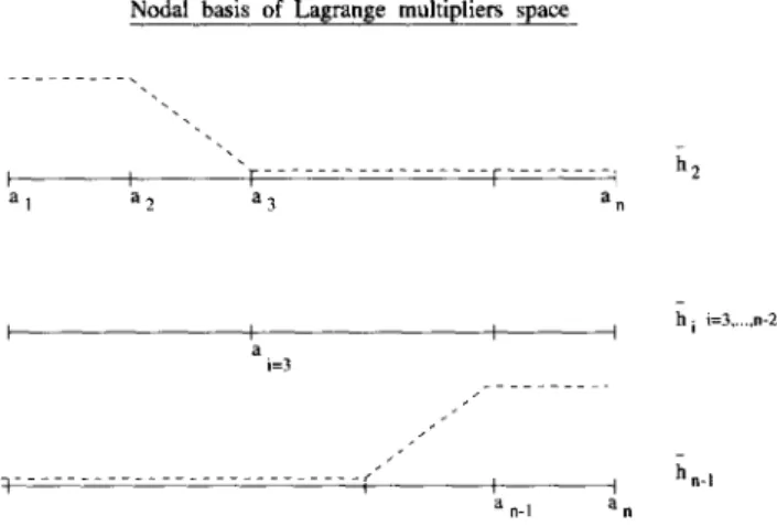
Nodal basis of Lagrange multipliers space

I I "~- . . . [- . . . I a I a 2 a 3 a n

h2

I t I a i = 3 . . . ( i i an_ I a n ~1 i i=3,...,n-2

Figure 2.1: Nodal basis of Lagrange multipliers space; the points ai are the vertices of the triangulation of ~k on F k'j

T h e discretized variational formulation of (1.5) is: F i n d u h E Y h

such that

K

(2.1)

~/vh E Yh' k~l

k ~ U h ' k ' ~ V h ' k

K

dx=k~l

~ = k fVh,kdx.

T h e problem (2.1) can be reformulated into a saddle point problem. Let

ah

be the s y m m e t r i c bilinear form on

Xh • Xh:

K

ah(Uh,Vh) = ~ f

VUh,k.VVh,k dx,

J ~ k

k~-I

and bh the bilinear form on

Xh • 17Vh:

(2.2)

bh(Vh,#h) =

~

fr

(Vh,k -- Vh,~),h. l < k < ~ < K k,t

We can associate to

ah

the linear o p e r a t o r

Ah

and to

bh

the linear o p e r a t o r

Bh

such t h a t

ah(Uh, Vh) -= (AhUh, Vh)

and

bh(Vh,Ph) = (BhVh,#h).

Therefore, the problem (2.1) a d m i t s a following saddle-point formulation:

Find the pair (Uh,)~h) in Xh X 17Vh such that

Ahuh + B~Ah = fh

(7)

3 T h e m o r t a r m e t h o d .

The m o r t a r m e t h o d corresponds to a particular choice for the gluing functions r over the non-mortar sides. We define each I ~ as a proper subspace of codimension 2 in W k'j. In case of first order approximation, it is the subspace

of all functions with zero slope on the elements including the end points. It is then an easy m a t t e r to make the following choice of basis

DEFINITION 3.1. In case of first order finite element spaces Xkh the basis functions -h of CV k'j are chosen as piecewise linear functions with zero slopes at the end points of interfaces, that vanish at any inner point of the discretization

ofrk,J except one (see Fig.

( 2 . 1 ) ) .

3.1 The interface matrix.

In this section, we will explain how to build the interface matrix Bh which

makes the correspondence between the degrees of freedom on interface and the degrees of freedom of the Lagrange multipliers. In all what follows, we consider the case of piecewise linear finite elements. We focus our attention on an interface

~/= Xox]y = ~ , y --/3[ between two subdomains ~t 1 and ~2 and we assume that

the side of ~2 is the m o r t a r one. We have to glue two subdomains with nonmatching grids on their common interface. Therefore, we have to solve:

ff

(ul - = 0

1

which can equivalently be written as

U 1 = O.

1

B1 ~32

We consider the shape functions of ui piecewise linear and the shape functions of r as already introduced in definition 3.1. Since the non-mortar side corresponds to domain 1, the gluing function r is defined on the grid of ~t 1

3.1.1 Computing

B1.

We denote by n the number of vertices of the triangulation of fll that belong to the interface. Basis functions corresponding to r are hk with k from 2 to n - 1 and basis functions corresponding to ul are hi.

9 I f k = 2 = : ~ h 2 = h l + h 2 .

9 I f k = 3 , . . . , n - 2 ~ - h k = h k . 9 I f k = n - l ~ h k = h n - l + h n .

(8)

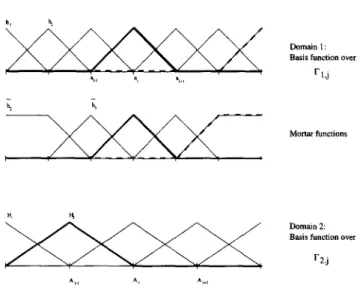
D o m a i n 1 :

Basis function over

F 1 j Mortar functions A H Ai Ai.~ D o m a i n 2: Basis f u n c t i o n over r2.j

Figure 3.1: Lagrange multipliers space.

T h e e v a l u a t i o n of B1 consists in c o m p u t i n g :

ia,, ~ ul(ai)hi-hk

,&

w i t h k from 2 t o n - 1 .

1 i = 1

W e r e m a r k t h a t B1 is a r e c t a n g u l a r m a t r i x w i t h n - 2 lines a n d n c o l u m n s , so t h a t t h e i n n e r values

ul(ai)i=2

. . . 2 are e n t i r e l y d e t e r m i n e d from t h e values of u z ( a l ) ,

ul(an)

a n d t h e c o m p l e t e set u2(y), y E (A1, ..., Am).

H o w to

i m p l e m e n t B I ? 9 E n d p o i n t s . 1. F o r i--- 1 = 0 i f j > 2 , = h i = _ _ a 2 - a l = _ _ a 2 - a l

1

2

2. Similarly, for i = n

i l ~ h~hj

: 0 i f j < n - 1 , = h n - - a n - a n - 1 n--1 2

(9)

MATCHING NONCONFORMING GRIDS

727 9 F o r i = 2 o r i = n - 1 1. F o r i = 2 ~a a'+ l h2-h2 i - - 1

f~i '~ h2-f~

fa a2

fa a3

=

h2

+ h22 = a2 - a :

a3 -- a2

, 2 2

+ ~

:

a3 -- a~

= h~h3 1 2

/_~ ( 1 _ ~ ) ( ~ _ x ) a 3 - - a 2

a a - - a 2 2 6 0 i f j > 3. 2. S i m i l a r l y for i = n - 1. 9 In n e r p o i n t s . ~ h & fo. ai + l hi-hi a i - 1 = 0 i f j r i, i + 1 3 3 3

~al

~-:

_hi-hi+l-~

/_11

( ~ - - ~ ) ( ~ " ~ - ) a i + 1 2 - - a i

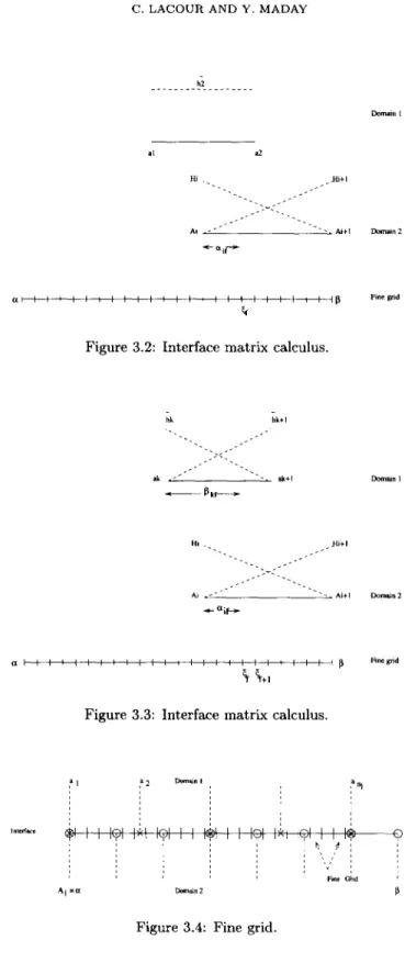
, _ 0 1 ~ 2 ai - ai-1 ai+l - ai 1 2 1 2 a i -- a i - 1 a i + l -- a i a i + l -- a i - 1 a i + l -- a i 3.1.2 Computing 132.

Basis f u n c t i o n s c o r r e s p o n d i n g t o r are t h e s a m e as before hk for k = 2 , . . . , n - 1 a n d p r o l o n g a t e d b y 0 over F 2,m for some m in case F 1,n does not coincide w i t h F 2,m. W e set F 2,m = ] a , ~I- Basis f u n c t i o n s c o r r e s p o n d i n g t o u2 a r e Hi as is i l l u s t r a t e d in Fig. 3.2.

T h e t e c h n i q u e now consists in i n t r o d u c i n g a finer grid of p o i n t s (~/)t=l ... F on t h e interface as shown in Fig. 3.4.

~ U2~k(X) dx

m

f <'+'

= H,(x)-hk(x) dx

f i=1

"]~f

(10)

728 c . LACOUR AND Y. MADAY

al a2

Hi . . ~ ~li+ I

< - a i f - ~

Figure 3.2: Interface matrix calculus.

Fine grid hk hk+l ak ak+l Dom~n 1 Hi . . - ~ l i + l Ai - ~ " - Ai+l a l l l ~ l t l l l l l l i q i l l l l l I I 1 1 ~

Figure 3.3: Interface matrix calculus.

Fine grid ,a I a 2 D~u~in I a nl ; [ '

li

, ~, ,4 , i V i ' Fine Ghd A I = ~ Domain 2 -Q Figure 3.4: F i n e grid.

(11)

MATCHING NONCONFORMING GRIDS 729 where k goes from 2 to n - 1 and where

9 n is the n u m b e r of points of the t r i a n g u l a t i o n of [21 and the interface. 9 m is the n u m b e r of points of the t r i a n g u l a t i o n of ~2 and the interface. 9 :f is the n u m b e r of points on the fine grid.

T h e integration over ]

~f~f+l[

is a p p r o x i m a t e d by a trapezoidal rule, we obtain:

u 2 e ( x )

dx -- ~ _ , ~ _ u 2 ( A , )

:I+l__ :.f

[H, h k ( : I ) - } - H i h k ( : f + l ) ]

f i=1

with k from 2 to n - 1.

H o w to i m p l e m e n t B2?

Hi-fk(~f) r 0 ~

~f E

[ A i - l , A i + l ] n [ a k - l , a k + l ] .

9 If k = 2 and ~I E [al,a2], the h2 is equal to 1 over [al,a2], and since ~i C [ A i - l , A i + l ] , ~ i f = I A i - ~II.

1 - (~iy if ~I E [Ai-1, Ai]

Hi-h2(~f) = 1 Ai - A i - 1 1 - ceil if { f E [Ai, A i + I ] . = 1 Ai+I -

Ai

9 I f k = 2 a n d ~ f E [a2,a3] or if k = n - 1 and ( f e [a~-2, a n - l ] or if 3 < k < n - 2 t h e n we set /3k f =

g~-~k(~f ) =

lak -- ~II

and

(1

if

~f C [ak-1, ak] n [Ai-1, A~]

and similar relations in other cases.

4 T h e F E T I m e t h o d .

T h e F E T I m e t h o d differs from the previous m o r t a r m e t h o d from the choice of the L a g r a n g e multipliers. Here the skeleton S is further d e c o m p o s e d since we consider the p a r t i t i o n

S -~- (,.Jl~_k<e<N~k~,

where we recall t h a t Fk~ is the segment such t h a t

Fke = ~k n - ~ .

Over each entity Fke a space of local polynomials is introduced with degree _<

nk,e.

(12)

7 3 0 C . L A C O U R A N D Y . M A D A Y

As for the mortar approach for the Lagrange multipliers, we have to glue two subdomains with non-matching grids on their interface. So, we have to satisfy the condition

~a an

(4.1) ( ~ - ~ : ) r : 0

1

where ul and u2 are the traces of finite element functions on S21 and D 2 and r are polynomials over the non-mortar Fie =

xo•

= c~, y = f~[, see Fig. 4.1:

i n t e r f a c e

m

- - (

r

c o a r s e mesh fine mesh m D m m X \ x : | " - . Trace of (p polynomial

Figure 4.1: Polynomial Lagrange multipliers.

(4.2) r

anY--aA-

al

1 ) .

Computation: The integral can equivalently be written as:

r - u 2 r = 0.

1

y _Y 9

B1 B2

The evaluation of each term is decomposed over each element

]ai,

ai+l[ of the interface

l(zo_

r

g l = ~ +

i = 2 ~ - 1 ,i a i

(4.3) = ~ ( / _ 1 1 1 - F x I x + l ,

] ai-ai_ldx

i=2

~ r L---~--(ai - ai-1) + ai-1

2 + f_: 1-

x_V r [--V

- ai) +ailai+12-aidx

) - -

and the integrals over each element are computed exactly by using a Gauss-type quadrature formula. A similar treatment is done for •2 based on the points

Ak.

The basis functions that are used to span the space of polynomials are the set of Legendre polynomials Ln.

(13)

MATCHING NONCONFORMING GRIDS 731 5 N u m e r i c a l e x p e r i m e n t s .

5.1 Generalities.

For mixed formulations, as the ones that are encountered in this type of method, it is well known that a crucial argument is related to the compatibility between the discrete space of Lagrange multipliers and the space of discrete subdomain solutions. In order to have a unique solution, it is important that the space of Lagrange multipliers is not too rich. This is expressed by the standard inf-sup condition recalled in the following hypothesis.

HYPOTHESIS 5.1 (LADYZHENSKAYA, BABUSKA AND BREZZI). Let us denote by Fk,~ any non-mortar edge of the subdomain ~k, we have:

inf sup ' >/3~ II#hl[ 2 89 ,

~hEWh vhCXh IJvhI[* -- (Hoo(Fk,D)

where the constant/3~ is > 0 but may depend on the discretization parameters.

Of course, in order to have an optimal approximation, this dependency of the inf-sup constant has to be as low as possible, the best being that /3~ is independent of the discretization parameter. For the Mortar method, it is proven that it is the case: the inf-sup condition is independent of the discretization parameter [4] and the optimality of the discrete method results. Actually, it is proven in [4] that the inf-sup condition holds on a smaller space for the v. Let us denote by Zh the subspace of Xh of elements that vanish on the mortars (and not on the nonmortars), then the following inf-sup condition is satisfied

(5.1) i n f s u p ~-~(k'~)fr~'~vkh#hds _>/3~ ((k~,~) :_~_ ) 1 / 2

REMARK 5.1. Any choice of space for the Lagrange multiplier as being a subspace of the original proposed space results also in a constant inf-sup condition. This is nevertheless at the price of a degradation of the approximation of the Lagrange multiplier s that actually pollutes the global solution.

For the FETI method, no theory is yet available but it is noticeable from the numerical point of view that the inf-sup constant is not independant of the discretization parameter, i.e the degree of the local Lagrange multipliers as is presented in the next section.

5.2 Numerical evaluation of the inf-sup condition.

This part deals with the relation between the eigenvalues of the algebraic system resulting from the implementation of the Shur dual method in the case of nonconforming grids and the inf-sup constant arising in the verification of the inf-sup condition.

(14)

732 C LACOUR AND Y. MADAY

Let us first consider the m o r t a r element method. Let ]/h be given in W h with

'/. ),I2

I ~ = 1 .

It is immediate to deduce from (5.1) t h a t another inf-sup condition then holds

inf sup }-~(k,e) Jr~,e h --

.hew,, .,,,~x,, IIv,,ll. ->/~ I1~"11~ _(Hoo(Pk,e))89 '

As already noticed in [14], the elements v~ E X h t h a t realize the s u p r e m u m in this inf-sup condition, i.e.,

V*t " h

sup ----

~.~x~

Ilvhll,

Ilvs

are collinear to the element ~ of X a solution of the problem

s

f

k k (k,~) JFk,e

where the solutions are locally chosen to be zero average over the flotting subdomains in order to ensure the uniqueness of the solution ~ . It follows t h a t

sup ' = ( ~ k _ h Jt~h ds

(k,t) Fk,~

If P denotes the vector in ] ~ M of nodal values of #h in the basis h, then it is immediate, from the previous definitions to note t h a t

E (BtkA-~'BkP'P) E

= f

((:;k

- Vh )#h ds. -.e

k (k,~) J Fk,t

Let us denote by

II~hll- 89 = /Y~s II~hll ~

89 ,

V

(k,e) (Hoo (Fk'e))

This provides the relation

r (v k - V~h)#h ds E ( k , f ) JFk,~ h inf sup .h~Wh

v,,~x,,

Ilvhll,ll,~hll- 89

= , / inf Y ~ ' k ( B t k A k l B k P ' P ) V P e ~ - II,uh(p)ll_}

(15)

MATCHING NONCONFORMING GRIDS 733

where #h (P) denotes the element of

Wh

the nodal values of which, by definition, are equal to P. Recalling that the matrix

BtkA-~lBk

is symmetric, it follows that

inf

E(BtkA;1BkQ,

Q ) : O/mi n

QC~tM'IIQIIe~(~M)=I k

where amin is the smallest eigenvalue of

~'~k BkAk Bk.

t -1 It is well known also from the equivalence of the norms over

Wh

given by the condensation of the mass matrix that, for any vector Q in ~ M ,

"Q"e2(~M) ~-- i~k, hk"Ph(O)l'2L2(rk,~ )

moreover, the standard imbeddings and the inverse inequalities over the finite element functions give

(5.2)

[I,h(Q)ll(Ho 89

<

II,h(Q)llL~(r~.~) _<

h;U211,h(Q)ll(Hoto(r~.m .

Finally, summing up the previous relations, we derive on the one hand that

c aX/r~min < inf sup

-

.~cw~ ~ x ~

Ilvhll,(E(k,~)h;lll~ll " ~.

.)u~

(Ho~o(rk,l)) ' and on the other hand

C ~ > inf sup #hEWh vhCXh hence "X 1/2 / Ilvhll. {E(k, )h; ll hlF , k

(H~(rk,e))']

~5 ~ O~min

where hmin stands for the smallest hk.

t --1

Similarly, we derive that the largest eigenvalue C~max of

BkA k Bk

satisfies cV hmax < sup sup

~ t h E W h ?2hEXh

/

\ :/a

(Hoo(rk,~)) /

and the expression on the right is upper bounded by a constant by using the standard trace theorems. This leads to the fact that ~max is upper bounded by a constant times h. These two expressions clearly yield that if ~ denotes the condition number of

BtkAklBk

then

Chm~x < - - .

(16)

0.8:

0.6

0., !

0.2

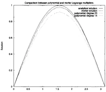
Comparison between polynomial and mortar Lagrenge multipliers

' ' ~ : : ~ ' analytical solution ~ ' / , : ( "%~ mortar solution ...

/..": '~',~ polynomial degree 23 ....

0.5 1 1.5 2 2.5 3

Figure 5.1: Solution with the Mortar method and the FETI method.

REMARK 5.2. Actually it is reasonable to think that for elements that realize the infimum in the inf-sup constant, the inverse inequality (5.2) scales like h -1/2,

meaning that (in case, for simplification, where hrnin and hm~x are comparable)

fq m__in

(5.3) t3~ ~_,JV h-2 "

It is also reasonable to think that C~ma x scales exactly as a constant times h (indeed it is lower bounded by the value of frk.~ Vh#h ds/(]lVh[[.[[phl[) obtained

for ~h being an approximation of a sin wave and Vh being an approximation of

an harmonic extension of the sin wave).

These two heuristic statements come in accordance with the numerical exper- iments reported in Figs. 5.3, 5.4, where amin is proven to scale like h 2 and ~ as

c/h.

Let us now consider the polynomial F E T I approach. If the Legendre basis is chosen to represent the Lagrange multiplier, the only difference with respect to the previous analysis is in the relation between the H - 1 / 2 - n o r m of #N and the ~2-norm of its coefficients. Since this g2-norm is equivalent to the L2-norm of # g , the only element comes from the inverse inequality (5.2) yielding

g 2

_<c--

The numerical experiment reported in Fig. 5.2 shows that the condition number a grows exponentially fast with the degree N of the polynomial Lagrange multiplier so that the inf-sup constant has a very bad behaviour.

(17)

MATCHING

NONCONFORMING

GRIDS

735

o .J

8

4.5 Condition number of the dual matrix

polynomial Lagrsnge multipliers - - Mortar Lagrsnge multipliers 4 3.53 2.5

I

2 1.51 ~

0.5

0

₅ ₁₀ ₁₅ ₂₀ Degree of polynomial

Figure 5.2: Behaviour of the Dual matrix' condition number versus the degree of polynomial, same mesh as in Fig. 5.1, the horizontal line corresponds to the mortar Lagrange multipliers.

250

200

Beheviour of condition number versus the mesh size

.~ 150

o IO0

50

1H 22 H 3 44 H 5 6 7 ~H

H

Figure 5.3: Mortar Lagrange multipliers: behaviour of the Dual matrix' condition number versus the mesh size, same mesh as in figure 5.1

(18)

736 C. L A C O U R A N D Y. M A D A Y

Behaviour of beta versus the mesh size

0.1 0.09 0.08 0.07 0.06 i 0.05 0.04 0.03 0.02 0.01 0 1 H 0,8 0.6 H/2 0.4 H/4 0.2 H/8 H

Figure 5.4: Mortar Lagrange multipliers: behaviour of f~ versus the mesh size, same mesh as in figure 5.1

REMARK 5.3. The influence of this bad inf-sup condition is not only noticeable on the approximation result but yields also a degradation of the performance of the algorithms for solving the problem. In order to circumvent this drawback it has been proposed in [10] to use "piecewise (relatively) low order polynomial" instead of full polynomials. The F E T I method then gets closer to the m o r t a r method.

In addition, the verification of the inf-sup condition is not certified and is a prerequisite of the method. To verify this condition, the Lagrange multiplier space should not be too rich. But, the less rich the space is, the less accurately the relation B i u i - B 2 u 2 = 0 is verified. In practice, it is difficult to check whether this condition is satisfied or not. Therefore, it is recommended to start with low order approximations of ~ and refine them. The rule of t h u m b consists in increasing the degree of polynomial N until N - 1 is less t h a n the number of inner degrees of freedom.

We compare now the Mortar Element method with the F E T I m e t h o d with polynomial Lagrange multipliers. We study the problem given in (1.1) on a square with f = 2 sin(x) sin(y). The analytical solution is then u = sin(x) sin(y). In Fig. 5.1 we have plotted a section of the numerical solution obtained with the same finite element methods over each subdomain and with different Lagrange functions. The domain is a square, decomposed into 4 (2 x 2) squares. Each square is provided with a quadrangulation: the two upper with 24 x 24 elements, the two lower with 32 x 32 elements. The m o r t a r results are obtained by using the choice advocated in section 3 (the gluing functions are on the coarser mesh, i.e., with 24 elements) and the polynomial results are obtained by using local polynomials with degree 23 so t h a t the dimension of the Lagrange space

(19)

M A T C H I N G N O N C O N F O R M I N G G R I D S 737

is the same. (As an illustration of the rule of thumb, we increase the degree of polynomial until N = 23 and for N = 24 we remark that the system is not invertible.)

We do not pretend t h a t this simple numerical example is a definitive statement on the compared qualities of the F E T I and the Mortar approaches. Nevertheless, it is in concordance with the evaluation of the inf-sup condition. W h a t we claim overall is t h a t the numerical results presented in this section constitute a definitive answer as regards the evaluation of the inf-sup condition and the bad condition number of the resulting algebraic system.

6

Conclusions.

In this paper, we have compared two different approaches for the matching of nonconforming finite element methods: the Mortar m e t h o d and the polynomial F E T I method. We have presented t h e m in a unified version and focussed on the differences t h a t reduce to be only on the choice of the Lagrange multiplier space t h a t allow to glue together the different meshes. We have pointed out that the choice of m o r t a r method is more appropriate as it allows to

9 certify t h a t the compatibility condition between the discrete spaces is satisfied

9 provide an inf-sup condition t h a t is independent of the discretization parameter

9 lead to an algebraic system with well-conditioned matrices.

This is the reason why we have preferred this choice for the generalization to more complex situations. The already good condition number of the matrix is improved by developing preconditioners in the same spirit as the one proposed in [17]. Note t h a t a hierarchical basis for the m o r t a r space has also been introduced t h a t improved even more the convergence of the iterative resolution of the problem. We refer to [19] and [12] for the presentation of these techniques.

Acknowledgement.

The authors want to express their thanks to C. Farhat and F. X. Roux for advice and helpful discussions.

R E F E R E N C E S

1. G. S. Abdoulaev, Y. Achdou, Yu. A. Kuznetsov, and O. Pironneau, The numerical implementation of the domain decomposition method with mortar finite elements for a 3D problem, preprint.

2. A. Agouzal and J. M. Thomas, Une mdthode d'dldments finis hybrides en ddcom- position de domaines, M2AN, 29:6 (1996), pp. 749-764.

3. Y. Achdou and Y. Maday, review article in preparation.

4. F. Ben Belgacem, The mortar finite element method with Lagrange multipliers,

(20)

5. F. Ben Belgacem and Y. Maday, Coupling spectral and finite element discretizations for second order elliptic three dimensional equations, preprint.

6. C. Bernardi, Y. Maday, and A. T. Patera, A new nonconforming approach to do- main decomposition: the mortar element method, in Coll~ge de France Seminar, H. Brezis, and J.-L. Lions, eds., Pitman, 1990.

7. F. Brezzi and D. Marini, A three fields domain decomposition method, in Contempo- rary Mathematics, A. Quarteroni, J. Periaux, Y. A. Kuznetsov, and O. B. Widlund, eds., Vol 157, 1994, pp. 27-34.

8. L. Cazabeau, Mdthodes multi-domaines pour la rdsolution des dquations de Navier- Stokes en simulation numdrique directe, PhD. thesis in preparation.

9. C. Farhat and M. Geradin, Using a reduced number of Lagrange multipliers for as- sembling parallel incomplete field finite element approximations, Comput. Methods Appl. Mech. Engrg., 97 (1992), pp. 333-354.

10. C. Farhat and F. X. Roux, A method of finite element tearing and interconnecting and its parallel solution algorithm, Internat. J. Numer. Meth. Engrg., 32 (1991), pp. 1205-1227.

11. D. E. Keyes and J. Xu, Domain decomposition methods in scientific and engineer- ing computing, in Proceedings of the Seventh International Conference on Domain Decomposition, The Pennsylvania State University, October 27-30, 1993. Contem- porary Mathematics, Vol 180, 1994.

12. C. Lacour, Iterative substructuring preconditioners for the mortar finite element method, in Proceedings of the Ninth International Conference on Domain Decom- position, Bergen, 1996, John Wiley & Sons, to appear.

13. P. Le Tallec, T. Sassi, and M. Vidrascu, Three-dimensional domain decomposition methods with nonmatching grids and unstructured coarse solvers, in Proceedings of the Seventh International Conference on Domain Decomposition, The Pennsylvania State University, October 27-30, 1993. Contemporary Mathematics, Vol 180, 1994, pp. 61-74.

14. Y. Maday, D. Meiron, A. T. Patera, and E. M. Rcnquist, Analysis of iterative methods for the steady and unsteady Stokes problem: Application to spectral element discretizations, SIAM J. Sci. Comput., 14:2 (1993), pp. 310-337.

15. Proceedings of the Eighth and Ninth International Conference on Domain Decom- position, John Wiley &: Sons, to appear.

16. P. A. Raviart and J. M. Thomas, Primal hybrid finite element methods for second order elliptic equations, Math. Comp., 31 (1977), pp. 391-413.

17. F. X. Roux, M~thode de dgcomposition de domaine it l'aide de multiplicateurs de Lagrange et application it la rdsolution en parall~le des dquations de l'dlasticitd lindaire, Ph.D. thesis, 1989, Universite Pierre et Marie Curie, Paris.

18. J. M. Thomas, Formulation mixte des dquations aux ddrivdes partielles du second ordre elliptiques, Ph.D. thesis, 1977, University Paris VI.

19. H. Yserentant, On the multi-level splitting of finite element spaces, Numer. Math., 49 (1986), pp. 379-412.