A GenEO Domain Decomposition method for Saddle Point problems

(1)

HAL Id: hal-02343808

https://hal.archives-ouvertes.fr/hal-02343808v4

Preprint submitted on 26 Apr 2021

HAL is a multi-disciplinary open access

archive for the deposit and dissemination of sci-entific research documents, whether they are pub-lished or not. The documents may come from teaching and research institutions in France or abroad, or from public or private research centers.

L’archive ouverte pluridisciplinaire HAL, est destinée au dépôt et à la diffusion de documents scientifiques de niveau recherche, publiés ou non, émanant des établissements d’enseignement et de recherche français ou étrangers, des laboratoires publics ou privés.

A GenEO Domain Decomposition method for Saddle

Point problems

Frédéric Nataf, Pierre-Henri Tournier

To cite this version:

Frédéric Nataf, Pierre-Henri Tournier. A GenEO Domain Decomposition method for Saddle Point problems. 2021. �hal-02343808v4�

(2)

A GenEO Domain Decomposition method

for Saddle Point problems

F. Nataf ∗1 _{and P.H. Tournier} †2 1,2

Sorbonne Université, CNRS, Université de Paris, Inria Equipe Alpines, Laboratoire Jacques-Louis Lions, F-75005 Paris, France,

April 26, 2021

We introduce an adaptive element-based domain decomposition (DD) method for solving saddle point problems defined as a block two by two matrix. The algorithm does not require any knowledge of the constrained space. We assume that all sub matrices are sparse and that the diagonal blocks are spectrally equivalent to a sum of positive semi definite matrices. The latter assumption enables the design of adaptive coarse space for DD methods that extends the GenEO theory [32] to saddle point problems. Numerical results on three dimensional elasticity problems for steel-rubber structures discretized by a finite element with continuous pressure are shown for up to one billion degrees of freedom.

1 Introduction

Solving saddle point problems with parallel algorithms is very important for many branches of scientific computing: fluid and solid mechanics, computational electromagnetism, inverse problems and optimization.

We are interested in domain decomposition (DD) methods since they are naturally well-fitted to modern parallel architectures. For specific systems of partial differential equations with a saddle point formulation, efficient DD methods have been designed, see e.g., [28, 23, 29] and [34] references therein. Also in [16], a GenEO coarse space is introduced for the P.L. Lions’ algorithm and its efficiency is mathematically proved for symmetric definite positive problems. In the above article, numerical experiments are conducted on three dimensional elasticity problems for steel-rubber structures discretized by a finite element with continuous pressure. Although the method works well in practice, the method lacks theoretical convergence guarantees and also demands the design of specific absorbing conditions as interface conditions. The method we propose in our article has a provable efficiency and bypasses the need for absorbing boundary conditions.

Here as in [26, 4, 9, 30], we consider the problem in the form of a two by two block matrix. Let m and n be two integers with m ă n. Let A n ˆ n SPD matrix and B be a sparse m ˆ n full rank matrix of constraints and C a m ˆ m non negative matrix (in particular, C “ 0 is allowed), we consider the following saddle point matrix:

A :“ ˆ A BT B ´C ˙ . (1)

When the kernel of matrix B is known, very efficient multigrid methods have been de-signed in the context of finite element methods, see e.g., [7, 19, 18, 2, 31, 14]. Without this knowledge, it is nevertheless also possible to design efficient geometric multigrid methods as in [11] where the fine mesh is obtained by several uniform mesh refinements.

Here we do not assume any knowledge on the kernel of matrix B and we work with arbitrary meshes. The following three factor factorization, see e.g., [5]:

ˆ A BT B ´C ˙ “ ˆ I 0 BA´1 _I ˙ ˆ A 0 0 ´pC ` BA´1BTq ˙ ˆ I A´1_BT 0 I ˙ , shows that solving the linear system with A can be performed by solving sequentially linear systems with A and one with the Schur complement C ` BA´1_BT_{. In order to build a} scalable method, we assume that all three matrices A, B and C are sparse and that A and C are the sum of positive semi definite matrices. This is easily achieved in finite element or finite volume contexts for partial differential equations. The latter assumption enables the design of adaptive coarse space for DD methods, see [10].

(4)

More precisely, in § 2, we recall the two-level additive Schwarz method denoted MA used to precondition the matrix A (the primal-primal block of the saddle point problem). Then in § 3, we introduce the operator PS :“ C ` BMA´1BT which is spectrally equivalent to the Schur complement S. Its preconditioning is studied in § 3.2. In § 4, we combine these different components to define in a compact way the parallel saddle point preconditioner. In § 5, we present weak and strong scaling experiments on large scale elasticity problems for steel-rubber structures discretized by a finite element with continuous pressure. These problems are highly heterogeneous since the Lamé-Poisson coefficients of the rubber are pE1, ν1q “ p1 ˆ 107, 0.4999qand those of the steel are pE2, ν2q “ p2 ˆ 109, 0.35q.

2 Preconditioning of matrix A

The sparse nˆn SPD matrix A is preconditioned by a two-level Schwarz type DD method: M´1 A :“ R T 0 pR0ART0q´1R0` N ÿ i“1 RT_i pRiARTi q´1Ri, (2) where R0 is full rank dimpV0q ˆ n where V0 denotes the space spanned by the columns of RT

0. The following assumptions are crucial to ensure the final method is scalable: Assumption 2.1 (dimension and structure of the coarse space)

• The coarse space dimension, dimpV0q, is OpN q typically 10-20 times N . • The coarse space is made of extensions by zero of local vectors.

Using the GenEO method [32], it is possible to fix in advance two constants 0 ă λmă 1 ă λM and then build a coarse space V0 such that M_A´1 is spectrally equivalent to A´1:

1 λM M´1 A ď A ´1 ď 1 λm M´1 A , (3)

The dimension of the coarse space V0 is typically proportional to the number of subdo-mains. This corresponds to Assumption 2.1. More precisely, for each subdomain 1 ď i ď N, let Di be a non negative diagonal matrix that defines a discrete partition of unity, i.e.:

N ÿ

i“1

RT_i DiRi“ I , and AN eu

i be a symmetric semi-definite positive matrix such that for the maximum multi-plicity of the intersection of subdomains denoted k1, we have:

N ÿ

i“1

RT_i AN eu_i Ri ď k1A . (4)

Then, the GenEO eigenvalue problem is local to each subdomain and reads: Find pλik, Vikq P R ˆ RrankpRiq such that:

pDiRiARTi Diq Vik “ λikAN eui Vik. (5) Let τ ą 0 be a positive threshold, the coarse space is the vector space spanned by the vectors RT

i DiVik for all λik ą τ. Then inequality (3) holds with λm :“ p1 ` k1τ q´1 and λM :“ k0 where k0 is the maximal number of neighbours of a subdomain including itself.

Our aim in the next section is to precondition the Schur complement ´S of matrix A (eq. (1)) where

(5)

This is achieved by a series of spectrally equivalent matrices or preconditioners, the first one being PS defined as follows:

PS :“ C ` B MA´1B

T ₍₇₎

and the final one being N´1

S introduced in § 3.3, see eq. (25). Finally in § 4.2 we will introduce the preconditioner of the saddle point matrix A.

3 Schur complement preconditioning

3.1 First spectrally equivalent preconditioner

Note that PS is by definition a sum of N ` 2 positive semi definite matrices PS :“ B RT0 pR0ART0q´1R0BT ` C `

N ÿ

i“1

BRT_i pRiARiTq´1RiBT . (8)

Since B is a sparse matrix, it is interesting to introduce, for all 0 ď i ď N, ˜Rithe restriction operator on the support of =pB RT

i q so that ˜

R_iTR˜iBRTi “ BRTi . (9)

Then by defining for 0 ď i ď N, ˜

Bi :“ ˜RiB RiT, the operator PS is rewritten as

PS :“ ˜RT0B˜0pR0ART0q´1B˜T0R˜0 ` C ` N ÿ i“1 ˜ RT_i B˜ipRiARTi q´1B˜iTR˜i. (10)

We consider a partition of unity on H :“ Rm_{defined with local diagonal matrices p ˜}_D

iq1ďiďN P RdimpImpB RTiqqˆdimpImpB RTiqq: N ÿ i“1 ˜ RT_i D˜iR˜i “ IH.

Remark 3.1 This partition of unity exists since

B “ N ÿ i“1 BRT_i DiRi“ N ÿ i“1 ˜ RT_i R˜ipB RTi DiRiq is full rank.

We make the following assumption

Assumption 3.1 There exist symmetric positive semidefinite matrices p ˜Ciq1ďiďN such that for some constant ˜k1

C ď N ÿ i“1 ˜ RT_i C˜iR˜iď ˜k1C . (11) This assumption is not so restrictive. Indeed, for a minimization problem with constraints enforced exactly without penalization nor relaxation, we have C “ 0 and the assumption is automatically satisfied. Moreover, we have:

(6)

Proof If C is a diagonal matrix, it suffices to take ˜

Ci:“ ˜RiC ˜RTi D˜i,

which is a diagonal non negative matrix. Indeed, we then have for all P P Rm_: C P “ N ÿ i“1 C ˜R_iTD˜iR˜iP “ N ÿ i“1 ˜ RT_i p ˜RiC ˜RTi D˜iq ˜RiP .

Remark 3.2 Note also that in the finite element case it suffices to restrict to the sub-domains the variational form that defines C. In this case ˜k1 is the multiplicity of the intersections of the subdomains used to define the ˜Ci’s.

Let us define the operator MS as the sum of a non local but low rank matrix S0: S0:“ ˜R0TB˜0pR0ART0q´1B˜0TR˜0,

and of S1 which is a sum of N local positive semi definite matrices: S1 :“ N ÿ i“1 ˜ RT_i p ˜Ci` ˜BipRiARTi q´1B˜iTq ˜Ri, that is MS :“ S0` S1.

By Assumption 3.1, the operator MS is spectrally equivalent to PS which is also spectrally equivalent to S. Note that we may assume that S1 is invertible whereas it does not make sense for S0. Note that if it is not the case, since we build a preconditioner, S1 can be regularized by a small diagonal term with little effect on the efficiency of the preconditioner.

We consider next the construction of a preconditioner M´1

S1 to S1 leveraging the fact

that S1is a sum of symmetric semidefinite positive matrices. Let us stress that this property stems from the domain decomposition structure of the preconditioner for matrix A which apart from the coarse level is block diagonal.

3.2 Preconditioning of S1

It is well known that one level domain decomposition methods are in most cases not scal-able. Nevertheless, the study of a one-level method in § 3.2.1 enables the identification of a suitable coarse space that will be efficiently embedded in a scalable two-level domain decomposition method in § 3.2.2.

Our studies of the spectrum of the DD preconditioners are based on the Fictitious Space lemma which is recalled here, see [27] for the original paper and [15] for a modern presentation.

Lemma 3.2 (Fictitious Space Lemma, Nepomnyaschikh 1991) Let H and H_D be two Hilbert spaces, with the scalar products denoted by p¨, ¨q and p¨, ¨qD. Let the symmetric positive bilinear forms a : H ˆ H Ñ R and b : HD ˆ HD Ñ R, generated by the s.p.d. operators A : H Ñ H and B : HD Ñ HD, respectively (i.e. pAu, vq “ apu, vq for all u, v P H and pBuD, vDqD “ bpuD, vDq for all uD, vD P HD). Suppose that there exists a linear operator R : HD Ñ H that satisfies the following three assumptions:

(7)

(ii) Continuity of R: there exists a positive constant cR such that

apRuD, RuDq ď cR¨ bpuD, uDq @uD P HD. (12) (iii) Stable decomposition: there exists a positive constant cT such that for all u P H there

exists u_D P HD with RuD “ u and

cT ¨ bpuD, uDq ď apRuD, RuDq “ apu, uq . (13) We introduce the adjoint operator R˚ _{: H Ñ H}

D by pRuD, uq “ puD, R˚uqD for all uD P HD and u P H.

Then, we have the following spectral estimate cT ¨ apu, uq ď a`RB´1R˚Au, u

˘

ď cR¨ apu, uq , @u P H (14) which proves that the eigenvalues of operator RB´1_R˚_{A are bounded from below by c}

T and from above by cR.

The Fictitious Space Lemma (FSL) can also conveniently be related to the book [34]: the first assumption corresponds to equation (2.3), page 36 where the global Hilbert space is assumed to satisfy a decomposition into subspaces, the second assumption is related to Assumptions 2.3 and 2.4, page 40 and the third assumption corresponds to the Stable de-composition Assumption 2.2 page 40.

3.2.1 One-level DD for S₁

As in [10] chapter 7, we begin with a one-level Neumann-Neumann type DD method defined in terms of the Fictitious Space Lemma (FSL). This study will be the basis for constructing the two-level preconditioner in § 3.2.2. Recall the formula for the one-level preconditioner M_S´1 1,1 for S1: M´1 S1,1:“ N ÿ i“1 ˜ R_iTD˜ip ˜Ci` ˜BipRiARiTq´1B˜iTq:D˜iR˜i, (15) where the superscript : denotes a pseudo inverse in case the operator in brackets is not invertible. For sake of simplicity, we assume that they are invertible so that the following framework enables the study of MS1,1 with the fictitious space lemma. Let

H :“ Rm and let a be the following bilinear form:

a : H ˆ H Ñ R apP, Qq :“ pS1P, Qq . Let

HD :“ ΠNi“1Rrankp ˜Biq, and b be the following bilinear form:

b : HDˆ HD Ñ R bppPiq1ďiďN, pQiq1ďiďNq :“ N ÿ i“1 p p ˜Ci` ˜BipRiARTi q´1B˜Ti q Pi, Qiq . (16) We define R: R : HD Ñ H pPiq1ďiďN ÞÑ řN i“1R˜Ti D˜iPi. We now check the three assumptions of the FSL.

(8)

Surjectivity of R For any P P H, we have: P “ N ÿ i“1 ˜ RT_i D˜iR˜iP , so that P “ Rpp ˜RiPq1ďiďNq . (17)

Continuity of R On one hand, we have using k₀ the number of neighbours of a subdo-main (including itself), k0 :“ max1ďiďN#Opiqwhere Opiq :“ t1 ď j ď N | ˜RiD˜iS1D˜jR˜Tj ‰ 0u: apRpPq , RpPqq “ }přN_i“1R˜T_i D˜iPiq}2aď k0 řN i“1} ˜RTi D˜iPi}2a “ k0p ´ ř jPOpiqR˜Tjp ˜Cj` ˜BjpRjARTjq´1B˜Tjq ˜Rj ¯ ˜ RT_i D˜iPi, ˜RiTD˜iPiq . On the other hand, we have by definition:

bpP , Pq “ N ÿ i“1 p p ˜Ci` ˜BipRiARTi q´1B˜iTq Pi, Piq . We can take: cR:“ max 1ďiďN_P max iPRrankp ˜Biq př_jPOpiqR˜iR˜jTp ˜Cj ` ˜BjpRjARTjq´1B˜jTq ˜RjR˜Ti D˜iPi, ˜DiPiq p p ˜Ci` ˜BipRiARTi q´1B˜iTq Pi, Piq , (18) but we have no control on cR which may be large. This motivates the introduction of a spectral coarse space in § 3.2.2 with the generalized eigenvalue problem (19) .

Stable decomposition Let P P H, we start from its decomposition (17) and estimate its b-norm

bpP , Pq “ řN_i“1p p ˜Ci` ˜BipRiAR_iTq´1B˜T_i q ˜RiP , ˜RiPq “ apP , Pq , so that we can take cT “ 1which is an optimal value.

3.2.2 Two-level DD for S₁

In order to control the value of cRdefined above, we introduce two two-level preconditioners. The first one is similar to what is done for Schur complement methods in [10, § 7.8.3, page 197] or in [33]. The second one is a cheaper lightweight version of the former but then not with a full control of its spectrum. In practice, in our numerical experiments both methods perform similarly in terms of iterations counts and thus with an advantage in terms of elapsed time for the second preconditioner. For both two-level methods, the generalized eigenvalue value problem in each subdomain 1 ď i ď N to be solved to build the coarse space is inferred from the definition of the constant cR in eq. (18):

˜ DiR˜i ´ ř jPOpiqR˜jTp ˜Cj` ˜BjpRjARTjq´1B˜jTq ˜Rj ¯ ˜ RT_i D˜i Pi k “ λi kp ˜Ci` ˜BipRiARTi q´1B˜iTq Pi k. (19) It can be solved in Op1q communications. The coarse space is defined as follows. Let τS1 be a user-defined threshold; for each subdomain 1 ď i ď N, we introduce a subspace

˜

Wi Ă Rrankp ˜Biq:

˜

(9)

Then the coarse space ˜W0 is defined (with some abuse of notation) ˜ W0 :“ à 1ďiďN ˜ RT_i D˜iW˜i.

Let ZS1 be a rectangular matrix whose columns span the coarse space ˜W0. Let ˜P0 be the

S1 orthogonal projection from Rm on ˜W0 whose formula is ˜ P0 “ ZS1pZ T S1S1ZS1q ´1_ZT S1S1. (21)

In order to avoid a too cumbersome analysis, we make the following assumption:

Assumption 3.2 We assume that for all subdomains 1 ď i ď N , ˜Ci` ˜BipRiARTi q´1B˜iT is invertible.

Finally, the first preconditioner for S1 reads M_S´1 1 :“ ZS1pZ T S1S1ZS1q ´1_ZT S1 ` pI ´ ˜P0q ˆ ´ řN i“1R˜Ti D˜ip ˜Ci` ˜BipRiARTi q´1B˜iTq:D˜iR˜i ¯ pI ´ ˜PT 0 q . (22) If Assumption 22 is not satisfied for some subdomain i, we should incorporate the kernel of ˜Ci ` ˜BipRiARTi q´1B˜iT in the coarse space and make use of a pseudoinverse in the definition of the preconditioner as it is done for the FETI method, see [13] or [10] § 7.8.2 and references therein.

Recall that from [10] chapter 7, we have for α :“ maxp1, k0

τ_S1q: 1 αM ´1 S1 ď S ´1 ď M_S´1₁ .

A careful implementation of (22) requires two coarse solves. In order to simplify the application of M´1

S1 , we can save one coarse solve by proposing an alternative definition of

preconditioner M´1

S1 without the global projection ˜P0. We directly define it using the FSL

framework. We keep definitions for H and a from the beginning of § 3.2.1. But now the space HD is defined as:

HD :“ RrankpZS1qˆ ΠNi“1Rrankp ˜Biq,

the operator R is defined using for 1 ď i ď N the p ˜Ci ` ˜BipRiARTi q´1B˜iTq orthogonal projections ξi on ˜Wi and parallel to SpantPi k | λi k ď τS1u :

R : HD Ñ H

pPiq0ďiďN ÞÑ ZS1P0`

řN

i“1R˜Ti D˜ipI ´ ξiqPi, and b is the following bilinear form:

b : HDˆHD Ñ R , bppPiq0ďiďN, pQiq0ďiďNq :“ pS1ZS1P0, ZS1Q0q`

N ÿ

i“1

p p ˜Ci` ˜BipRiARTi q´1B˜iTq Pi, Qiq . We now check the three assumptions of the FSL.

Surjectivity of R For any P P H, we have:

P “ N ÿ i“1 ˜ RT_i D˜iξiR˜iP ` N ÿ i“1 ˜ RT_i D˜ipI ´ ξiq ˜RiP .

Note that since the first sum belongs to ˜W0, there exists P0 such that řN_i“1R˜iTD˜iξiR˜iP “ ZS1P0. Then, we have:

(10)

Continuity of R For P P HD we have: apRpPq , RpPqq “ pS1RpPq , RpPqq ď 2 ppS1ZS1P0, ZS1P0qq ` pS1 řN i“1pI ´ ξiq ˜RiTD˜iPi, řN i“1pI ´ ξiq ˜RiTD˜iPiqq ď 2 ppS1ZS1P0, ZS1P0qq ` k0 řN i“1pS1pI ´ ξiq ˜RTi D˜iPi, pI ´ ξiq ˜RTi D˜iPiqq ď 2 ppS1ZS1P0, ZS1P0qq ` k0τS1 řN i“1pp ˜Ci` ˜BipRiARiTq´1B˜iTqPi, Piqq ď 2 maxp1, k0τS1q bpP , Pq ,

so that we can take cR“ 2 maxp1, k0τS1qand we lose only a factor of 2 compared to eq. (22).

Stable decomposition Let P P H, we start from its decomposition (23) and estimate its b-norm bpP , Pq “ pS1 řN i“1R˜Ti D˜iξiR˜iP, řN i“1R˜Ti D˜iξiR˜iPq `řN_i“1p p ˜Ci` ˜BipRiAR_iTq´1B˜iTq ˜RiP , ˜RiPq “ pS1 řN i“1R˜Ti D˜iξiR˜iP, řN i“1R˜Ti D˜iξiR˜iPq ` apP , Pq ď pγ ` 1q apP , Pq , where γ :“ max P pS1 řN i“1R˜Ti D˜iξiR˜iP, řN i“1R˜Ti D˜iξiR˜iPq pS1P , Pq . We can take cT :“ 1{p1 ` γq but we have no estimate on γ.

Finally, the explicit form of this alternative preconditioner reads: M´1 S1 :“ ZS1pZ T S1S1ZS1q ´1_ZT S1 ` ´ řN i“1R˜Ti D˜ipI ´ ξiqp ˜Ci` ˜BipRiARTi q´1B˜iTq:pI ´ ξTi q ˜DiR˜i ¯ . (24)

Note that the application of M´1

S1 can be done using only sparse solvers since solving a

linear system with a local Schur complement

p ˜Ci` ˜BipRiARTi q´1B˜iTqPi “ Gi,

amounts to solving an augmented sparse system which has the form of a local saddle point system: ´ ˆ RiARTi B˜iT ˜ Bi ´ ˜Ci ˙ ˆ Ui Pi ˙ “ ˆ 0 Gi ˙ .

3.3 Final Preconditioner for the Schur complement

From the spectrally equivalent preconditioner MS1 to S1, we define NS a spectrally

equiv-alent preconditioner to MS and thus to S as well:

NS :“ S0` MS1. (25)

We now consider the application of the preconditioner NS, that is for some right hand side G P Rm, the solving in P of the following system:

NSP “ G , (26)

by a Krylov solver with M´1

(11)

4 Recap

4.1 Setup for the Schur complement preconditioner

We have a setup phase which is composed of: 1. Build the two-level preconditioner M´1

A for A, see eq. (2), 2. Build the two-level preconditioner M´1

S1 for S1, see eq. (22).

Once the setup is complete, applying preconditioner N´1

S can be performed following Algorithm 1

Algorithm 1 N_S´1 matvec product INPUT: G P Rm _{OUTPUT: P “ N}´1

S G

1. Solve eq. (26) in P by a Krylov method with M´1

S as preconditioner.

4.2 DD solver for the saddle point system

We now consider the solving of the saddle point problem: ˆ A BT B ´C ˙ ˆ U P ˙ “ ˆ FU FP ˙ (27) by Algorithm 2 whose Step 3 demands the matrix-vector product with matrix C `BA´1_BT which is done by an iterative solve for matrix A´1. In order to avoid such nested loops, Algorithm 2DD saddle point solver

INPUT: ˆ FU FP ˙ P Rn`m OUTPUT: ˆ U P ˙ the solution to (27). 1. Solve AGU “ FU by a PCG with MA´1 as a preconditioner

2. Compute GP :“ FP ´ B GU 3. Solve pC ` BA´1_BT

qP “ ´GP by a PCG with N_S´1 as a preconditioner, see Algo-rithm 1

4. Compute GU :“ FU´ BTP

5. Solve AU “ GU by a PCG with M_A´1 as a preconditioner

block solvers have been developed, see [26, 4, 9, 36]. Following [36], nested loops are not needed when preconditioning the original system (1) by P´1 _{where P is an inexact block} factorization: P :“ ˆ MA B ´NS ˙ ˆ I M´1 A BT I ˙ (28) or a slightly different but symmetric variant of it introduced in eq. (2.5) of [36]:

P :“ ˆ I BM´1 A I ˙ ˆ MAp2 MA´1´ Aq´1MA ´NS ˙ ˆ I M_A´1BT I ˙ . (29) Note that in both cases, the inverses of P are computable easily in our framework.

5 Numerical experiments

In this section, we perform 3D experiments to illustrate the theory and the performance of the method. We are interested in a heterogeneous elasticity problem with nearly incom-pressible material typically rubber-steel structures. First, we recall the definition of the coefficients and the corresponding variational formulation.

(12)

The mechanical properties of a solid are characterized by its Young modulus E and Poisson ratio ν, or alternatively by its Lamé coefficients λ and µ. They verify the following relations:

λ “ Eν

p1 ` νqp1 ´ 2νq and µ “ E

2p1 ` νq. (30)

For the discretization, we choose a continuous pressure space and take the lowest order Taylor-Hood finite element C0P 2 ´ C0P 1 whose stability is proved, see e.g., [6]. The domain Ω is a beam and the variational problem consists in finding puh, phq P Vh :“ P32X pH01pΩqq3ˆ P1 with Dirichlet boundary conditions on the four lateral faces and Neumann boundary conditions on the other two faces such that for all pvh, qhq P Vh

$ ’ & ’ % ş Ω2µεpuhq : εpvhqdx ´ ş Ωphdiv pvhqdx “ ş Ωf vhdx ´ş_Ωdiv puhqqhdx ´ ş Ω 1 λphqh “ 0. (31) Letting u denote the degrees of freedom of uh and p that of ph, the problem can be written in matrix form as:

ˆ A BT B ´C ˙ ˆ u p ˙ “ ˆ f 0 ˙ . (32)

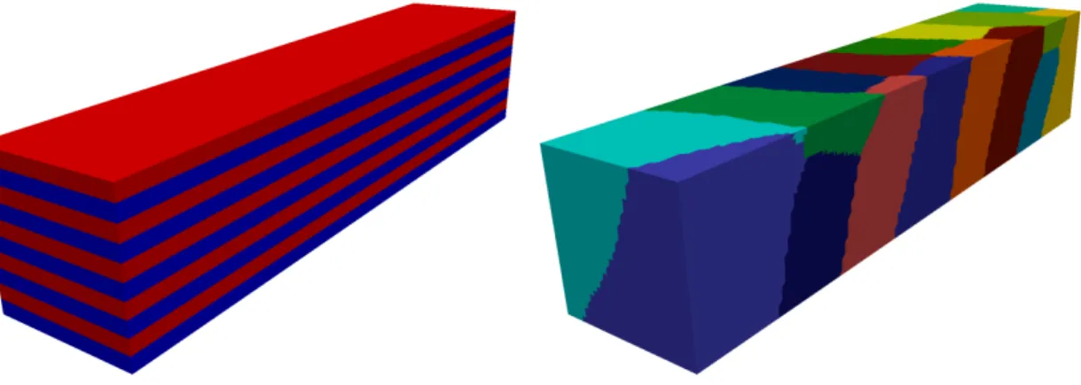
In the following numerical experiments, we consider a heterogeneous beam composed of 10 alternating layers of rubber material pE1, ν1q “ p1 ˆ 107, 0.4999q and steel material pE2, ν2q “ p2 ˆ 109, 0.35q, see Fig. 1.

5.1 Software, hardware, implementation details

In the following numerical experiments, the iteration counts assess the control of the con-dition number via the adaptive coarse spaces. We also report timings along with iteration counts. We also showcase the fact that the size of the GenEO coarse space adapts automat-ically to the difficulty of the problem at hand, for example when going from a homogeneous to a heterogeneous problem. We illustrate the efficiency of the method by performing weak and strong scalability tests, using the automatic graph partitioner Metis [22] for the sub-domain partitioning.

The problem is discretized and solved with the open-source parallel finite element soft-ware FreeFEM [17]. FreeFEM is domain specific language (DSL) where the problem to be solved is defined in terms of its variational formulation. Then the local matrices pAN eui q1ďiďN (see eq. (4)) and p ˜Ciq1ďiďN (see eq. (11)) are easily obtained by restricting the corresponding variational formulations to adequate local subdomains. Note that these matrices are different from the restriction of the global matrices A and C to the local degrees of freedom. The domain decomposition algorithm presented in this paper is implemented on top of the ffddm framework, a set of parallel FreeFEM scripts implementing Schwarz domain decomposition methods. ffddm already implements the GenEO method [32] for SPD problems, and its building blocks are designed to simplify the implementation and prototyping of new domain decomposition methods such as the saddle point solver pre-sented in this paper. The ffddm documentation is available on the FreeFem.org web page, see [35].

Numerical results are obtained on the french GENCI supercomputer Occigen, on the Haswell partition composed of 50544 cores of Intel Xeon E5-2690V3 processors clocked at 2.6 GHz. The interconnect is an InfiniBand FDR 14 pruned fat tree. We use Intel compilers, the Intel Math Kernel Library and Intel MPI.

(13)

As is usually done in domain decomposition methods, we assign one subdomain per MPI process. Our implementation is pure MPI and no multithreading is done ; we assign one MPI process per computing core. The mesh of the computational domain is partitioned using the automatic graph partitioner Metis [22] (see Figure 1). Local subdomain matrices are factorized by the sparse direct solver MUMPS [1]. Local eigenvalue problems are solved with Arpack [24] ; both libraries are interfaced with FreeFEM. GenEO coarse space matrices R0ART0 in (2) and ZST1S1ZS1 in (21) are assembled and factorized in a distributed manner

on a few cores (24 in most of the experiments) using the parallel solver MUMPS.

Figure 1: Heterogeneous beam composed of 10 alternating layers of rubber and steel. Coefficient distribution (left) and mesh partitioning into 16 subdomains by the automatic graph partitioner Metis (right).

For illustration purposes, we represent in Figure 2 (top) the eigenvalues of the local GenEO eigenvalue problems for both coarse spaces, V0 for A and ˜W0 for S1 (the former corresponding to eq. (5) and the latter to eq. (19)), for the heterogeneous beam problem with 16 million degrees of freedom, corresponding to the first row of Table 1. The figures show the inverse of the first 40 largest eigenvalues for 10 of the subdomains for the ex-periment corresponding to the first row of Table 1, so that the eigenvectors corresponding to the smallest values on the graphs (below the dashed line) will be selected to enter the coarse space. For comparison, we also solve the constant coefficient problem corresponding to an homogeneous steel (and compressible) beam and show the eigenvalues in Figure 2 (bottom).

We can see the effect of heterogeneities on the spread of eigenvalues for different sub-domains compared to the homogeneous case. In addition, we retrieve the 6 eigenvalues corresponding to the rigid body modes for A in the homogeneous case, and we see that we need a larger set of eigenvectors in order to build a robust coarse space in the heterogeneous case. Figure 2 also shows that there is no need for a coarse space for S1 in the compressible homogeneous case. A strong feature of the GenEO method is that relevant eigenvectors to enter the coarse space are selected automatically, adapting to the problem at hand and its spatial heterogeneity. Moreover, the robustness of the model does not rely on a specific partitioning, which allows the use of automatic graph partitioners such as Metis [22] or Scotch [8].

5.2 Parameters of the method

The method has a few parameters in play:

• The number of layers of mesh elements in the overlap region between subdomains is 2 for the velocity blocks (corresponding to Ri in (2)) and 4 for the pressure blocks (corresponding to ˜Ri in (10)). This corresponds to the minimum overlap that satisfies relation (9) for a symmetric construction of the overlap between subdomains.

(14)

0 0.1 0.2 0.3 0.4 0.5 0 5 10 15 20 25 30 35 40 1 / λ

steel/rubber - eigenvalues for A

0 0.2 0.4 0.6 0.8 1 0 5 10 15 20 25 30 35 40 1 / λ

steel/rubber - eigenvalues for S1

0 0.1 0.2 0.3 0.4 0.5 0 5 10 15 20 25 30 35 40 1 / λ

steel - eigenvalues for A

0 0.2 0.4 0.6 0.8 1 0 5 10 15 20 25 30 35 40 1 / λ

steel - eigenvalues for S1

Figure 2: Top: Heterogeneous steel and rubber beam. Bottom: Homogeneous steel beam. Inverse of the eigenvalues of the local GenEO eigenvalue problems for both coarse spaces, V0 for A (left) and ˜W0 for S1 (right), for 10 of the subdomains.

• For the heterogeneous beam problem, we set the threshold τA for selecting the local eigenvectors entering the coarse space V0 to 10 (corresponding to 0.1 on Figure 2, left). The threshold τS1 for selecting the local eigenvectors entering the coarse space

˜

W0 is set to 3.33 (corresponding to 0.3 on Figure 2, right).

5.3 Weak scalability test for heterogeneous steel and rubber beam

Here we present weak scalability results for the heterogeneous beam composed of 10 al-ternating layers of rubber pE1, ν1q “ p1 ˆ 107, 0.4999qand steel pE2, ν2q “ p2 ˆ 109, 0.35q. Local problem size is kept roughly constant as N grows, and the total number of dofs n goes from 16 million on 262 cores to 1 billion on 16800 cores. We use the original definition of M´1

S1 (22).

We report in Table 1 the iteration counts and computing times for the DD saddle point solver Algorithm 2. Note that in Algorithm 2 we replace PCG by right-preconditioned GMRES for step 3. The stopping criterion is a tolerance smaller than 10´5. Moreover, we use flexible GMRES, as we solve (26) inexactly using GMRES with a tolerance of 10´2 in order to apply N´1

S .

In order, columns correspond to: number of cores, number of dofs n, size of the coarse space for A dimpV0q, size of the coarse space for S1 dimp ˜W0q, setup time corresponding to the assembly and factorization of the various local and coarse operators, number of outer GMRES iterations, GMRES computing time, total computing time (setup + GMRES) and average number of inner GMRES iterations for each solution of (26). All timings are reported in seconds.

Iteration counts. We first discuss iteration counts. We see that outer iteration count remains stable, between 21 and 32. The inner iteration count is also stable and remains

(15)

#cores n dimpV0q dimp ˜W0q setup(s) #It gmres(s) total(s) #It NS´1 262 15 987 380 5 383 3 319 710.7 24 631.6 1342.3 11 525 27 545 495 9 959 2 669 526.6 21 519.5 1046.1 12 1 050 64 982 431 17 837 4 587 675.2 22 665.9 1341.1 11 2 100 126 569 042 32 361 7 995 689.2 25 733.8 1423.0 10 4 200 218 337 384 59 704 13 912 593.0 27 705.4 1298.4 10 8 400 515 921 881 141 421 25 949 735.8 32 1152.5 1888.3 10 16 800 1 006 250 208 260 348 41 341 819.2 29 1717.9 2537.1 12

Table 1: Weak scaling experiment for 3D heterogeneous elasticity: beam with 10 alternating layers of steel and rubber. Reported iteration counts and timings for DD saddle point algorithm 2.

around 11. We also observed (figures are not reported here) than the inner GMRES toler-ance of 10´2_{does not affect the outer iteration count compared to an accurate solution with} a stricter tolerance of 10´5_{, and allows a significant reduction in inner iteration count. For} example, 11 iterations on average instead of 28 on 1050 cores for the same outer iteration count of 22, leading to a decrease from 1178.2 to 665.9 seconds in GMRES timing.

Timings. In terms of setup timings, the computing time remains relatively stable, with roughly 15% increase for a factor of 64 in problem size. Around 60% of the setup time is spent in the solution of the eigenvalue problems (19) for S1.

The solution time stays relatively stable up to 4200 cores, where it starts to degrade. This can be related to the increased cost of the coarse space solves with matrices R0ART0 and ZT

S1S1ZS1 as their size increases: total time spent in coarse space solves is 14.7, 62.1

and 679.3 seconds on 262, 4200 and 16800 cores respectively. A possible improvement would be to use a multi-level method to solve the coarse problems iteratively.

5.4 Strong scalability test for heterogeneous steel and rubber beam

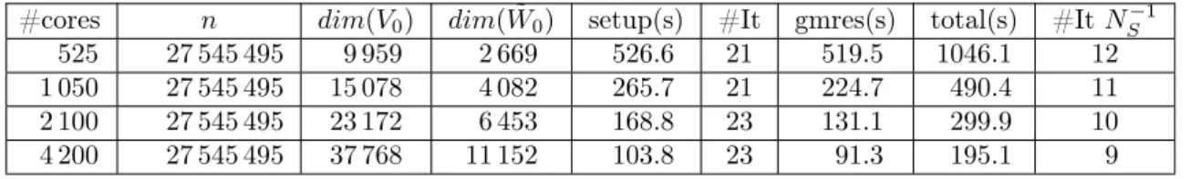
Strong scalability results for the heterogeneous beam composed of 10 alternating layers of rubber and steel are presented in Table 2. The problem size is 27.5 million and the strong scaling test ranges from 525 to 4200 cores. Iteration counts and computing times for the DD saddle point solver Algorithm 2 are reported.

#cores n dimpV0q dimp ˜W0q setup(s) #It gmres(s) total(s) #It NS´1

525 27 545 495 9 959 2 669 526.6 21 519.5 1046.1 12 1 050 27 545 495 15 078 4 082 265.7 21 224.7 490.4 11 2 100 27 545 495 23 172 6 453 168.8 23 131.1 299.9 10 4 200 27 545 495 37 768 11 152 103.8 23 91.3 195.1 9

Table 2: Strong scaling experiment for 3D heterogeneous elasticity: beam with 10 alternat-ing layers of steel and rubber. Reported iteration counts and timalternat-ings for DD saddle point Algorithm 2.

Iteration counts. Outer iteration count remains stable, with a slight increase from 21 to 23. Inner iteration counts remains also stable, even slightly decreasing from 12 to 9. Timings. We see that the setup timing decreases accordingly as the subdomains shrink in size, from 526.6 seconds on 525 cores to 103.8 seconds on 4200 cores; the speedup efficiency with respect to 525 cores ranges from 99% on 1050 cores to 63% on 4200 cores.

We see a similar trend for the solution time, ranging from 519.5 seconds on 525 cores to 91.3 seconds on 4200 cores ; the speedup efficiency with respect to 525 cores ranges from

(16)

116%on 1050 cores to 71% on 4200 cores. This decrease in efficiency can be explained by the increased relative cost of coarse space solves as subdomains get smaller: from 3% on 525 cores to 30% on 4200 cores. The added overlap also plays a greater role in the loss of efficiency as subdomains get smaller.

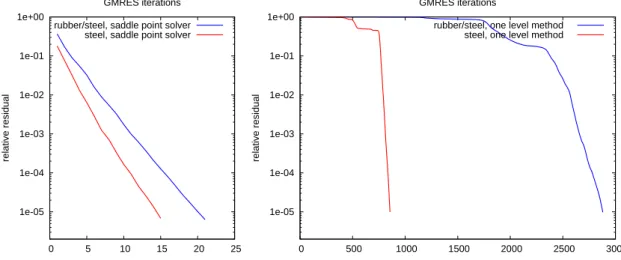
In Figure 3, we plot the convergence history of GMRES for both compressible homo-geneous and heterohomo-geneous steel-rubber cases with 27.5 million unknowns on 525 cores (left), with a comparison to the standard one-level Additive Schwarz Method (ASM) from PETSc [3] on the global problem (right), illustrating the difficulty of the test case at hand. Our saddle point solver needs 15 and 21 iterations to converge for the homogeneous and heterogeneous cases respectively, compared to 856 and 2880 for the one-level method, with significant undesired plateaux. For the same physical test case, iteration counts are better than in [16] but timings are not as good. As mentioned in the introduction, our method has the advantage of a provable convergence estimate and to not depend on the design of specific absorbing conditions for the elasticity system.

1e-05 1e-04 1e-03 1e-02 1e-01 1e+00 0 5 10 15 20 25 relative residual GMRES iterations rubber/steel, saddle point solver

steel, saddle point solver

1e-05 1e-04 1e-03 1e-02 1e-01 1e+00 0 500 1000 1500 2000 2500 3000 relative residual GMRES iterations

rubber/steel, one level method steel, one level method

Figure 3: GMRES convergence history of the saddle point solver (left) compared to the one-level Additive Schwarz Method (right) for the homogeneous steel beam and heterogeneous rubber/steel beam problems discretized with 27.5 million unknowns (corresponding to the first row of Table 2), on 525 cores.

6 Conclusion and outlook

Under the assumption that the diagonal block matrices of a saddle point problem are spectrally equivalent to a sum of positive semi definite matrices, we have introduced an adaptive domain decomposition (DD) method. For this, two coarse spaces are built by solving generalized eigenvalue problems, one for the primal unknowns and the second one for the dual unknowns. The robustness of the method was assessed on a notoriously difficult three dimensional elasticity problem for a steel-rubber structure discretized with continuous pressure.

Several issues deserve further investigations. First a multilevel method with more than two levels would enable even larger and possibly faster simulations. Also, the tests were performed with FreeFem scripts using the standalone ffddm [35] framework. The integration of the method in the C++/MPI library hpddm [21] could lead to faster codes and a more general diffusion of the saddle point preconditioner. In a different setting, the design of adaptive coarse space is strongly connected to multiscale finite element (MFE) methods (see e.g., [12, 20, 25] and references therein) and this work could be used in designing MFE methods for saddle point problem.

(17)

Acknowledgment

This work was granted access to the HPC resources of OCCIGEN@CINES under the allo-cation 2020-067730 granted by GENCI.

References

[1] Patrick R. Amestoy, Iain S. Duff, Jean-Yves L’Excellent, and Jacko Koster. A fully asynchronous multifrontal solver using distributed dynamic scheduling. SIAM J. Ma-trix Analysis and Applications, 23(1):15–41, 2001.

[2] Douglas N. Arnold, Richard S. Falk, and Ragnar Winther. Multigrid in h (div) and h (curl). Numerische Mathematik, 85(2):197–217, Apr 2000.

[3] Satish Balay, William D. Gropp, Lois Curfman McInnes, and Barry F. Smith. Efficient management of parallelism in object oriented numerical software libraries. In E. Arge, A. M. Bruaset, and H. P. Langtangen, editors, Modern Software Tools in Scientific Computing, pages 163–202. Birkhäuser Press, 1997.

[4] Michele Benzi, Gene H. Golub, and Jörg Liesen. Numerical solution of saddle point problems. Acta Numer., 14:1–137, 2005.

[5] Michele Benzi and Andrew J. Wathen. Some preconditioning techniques for saddle point problems. In Model order reduction: theory, research aspects and applications, volume 13 of Math. Ind., pages 195–211. Springer, Berlin, 2008.

[6] Franco Brezzi and Michel Fortin. Mixed and hybrid finite element methods, volume 15. Springer Science & Business Media, 2012.

[7] J Cahouet and J-P Chabard. Some fast 3d finite element solvers for the generalized stokes problem. International Journal for Numerical Methods in Fluids, 8(8):869–895, 1988.

[8] C. Chevalier and F. Pellegrini. PT-SCOTCH: a tool for efficient parallel graph order-ing. Parallel Computing, 6-8(34):318–331, 2008.

[9] Eric de Sturler and Jörg Liesen. Block-diagonal and constraint preconditioners for nonsymmetric indefinite linear systems. I. Theory. SIAM J. Sci. Comput., 26(5):1598– 1619, 2005.

[10] Victorita Dolean, Pierre Jolivet, and Frédéric Nataf. An Introduction to Domain Decomposition Methods: algorithms, theory and parallel implementation. SIAM, 2015. [11] Daniel Drzisga, Lorenz John, Ulrich Rude, Barbara Wohlmuth, and Walter Zulehner. On the analysis of block smoothers for saddle point problems. SIAM Journal on Matrix Analysis and Applications, 39(2):932–960, 2018.

[12] Yalchin Efendiev, Juan Galvis, and Thomas Y Hou. Generalized multiscale finite element methods (gmsfem). Journal of Computational Physics, 251:116–135, 2013. [13] Charbel Farhat and Francois-Xavier Roux. A method of Finite Element Tearing and

Interconnecting and its parallel solution algorithm. Int. J. Numer. Meth. Engrg., 32:1205–1227, 1991.

[14] Patrick E. Farrell, Lawrence Mitchell, and Florian Wechsung. An Augmented La-grangian Preconditioner for the 3D Stationary Incompressible Navier–Stokes Equa-tions at High Reynolds Number. SIAM J. Sci. Comput., 41(5):A3073–A3096, 2019.

(18)

[15] M. Griebel and P. Oswald. On the abstract theory of additive and multiplicative Schwarz algorithms. Numer. Math., 70(2):163–180, 1995.

[16] Ryadh Haferssas, Pierre Jolivet, and Frédéric Nataf. An additive schwarz method type theory for lions’s algorithm and a symmetrized optimized restricted additive schwarz method. SIAM Journal on Scientific Computing, 39(4):A1345–A1365, 2017.

[17] F. Hecht. New development in Freefem++. J. Numer. Math., 20(3-4):251–265, 2012. [18] R. Hiptmair. Multigrid method for Maxwell’s equations. SIAM J. Numer. Anal.,

36(1):204–225, 1998.

[19] Ralf Hiptmair. Multigrid method for h (div) in three dimensions. Electron. Trans. Numer. Anal, 6(1):133–152, 1997.

[20] Patrick Jenny, Seong H Lee, and Hamdi A Tchelepi. Adaptive multiscale finite-volume method for multiphase flow and transport in porous media. Multiscale Modeling & Simulation, 3(1):50–64, 2005.

[21] Pierre Jolivet and Frédéric Nataf. Hpddm: High-Performance Uni-fied framework for Domain Decomposition methods, MPI-C++ library. https://github.com/hpddm/hpddm, 2014.

[22] G. Karypis and V. Kumar. METIS: A software package for partitioning unstructured graphs, partitioning meshes, and computing fill-reducing orderings of sparse matrices. Technical report, Department of Computer Science, University of Minnesota, 1998. http://glaros.dtc.umn.edu/gkhome/views/metis.

[23] Axel Klawonn. An optimal preconditioner for a class of saddle point problems with a penalty term. SIAM Journal on Scientific Computing, 19(2):540–552, 1998.

[24] Richard B Lehoucq, Danny C Sorensen, and Chao Yang. ARPACK users’ guide: solution of large-scale eigenvalue problems with implicitly restarted Arnoldi methods, volume 6. SIAM, 1998.

[25] Chupeng Ma, Robert Scheichl, and Tim Dodwell. Novel design and analysis of gen-eralized fe methods based on locally optimal spectral approximations. arXiv preprint arXiv:2103.09545, 2021.

[26] Malcolm F. Murphy, Gene H. Golub, and Andrew J. Wathen. A note on precondi-tioning for indefinite linear systems. SIAM J. Sci. Comput., 21(6):1969–1972, 2000. [27] Sergey V. Nepomnyaschikh. Mesh theorems of traces, normalizations of function traces

and their inversions. Sov. J. Numer. Anal. Math. Modeling, 6:1–25, 1991.

[28] Joseph E Pasciak and Jun Zhao. Overlapping schwarz methods in h (curl) on polyhe-dral domains. Journal of Numerical Mathematics, 10(3):221–234, 2002.

[29] Luca F. Pavarino and Olof B. Widlund. Balancing Neumann-Neumann methods for incompressible Stokes equations. Comm. Pure Appl. Math., 55(3):302–335, 2002. [30] T. Rees and M. Wathen. An element-based preconditioner for mixed finite element

problems. SIAM Journal on Scientific Computing, 2020.

[31] S. Reitzinger and J. Schöberl. An algebraic multigrid method for finite element dis-cretizations with edge elements. Numerical Linear Algebra with Applications, 9(3):223– 238, 2002.

(19)

[32] Nicole Spillane, Victorita Dolean, Patrice Hauret, Frédéric Nataf, Clemens Pechstein, and Robert Scheichl. Abstract robust coarse spaces for systems of PDEs via generalized eigenproblems in the overlaps. Numer. Math., 126(4):741–770, 2014.

[33] Nicole Spillane and Daniel Rixen. Automatic spectral coarse spaces for robust finite element tearing and interconnecting and balanced domain decomposition algorithms. Internat. J. Numer. Methods Engrg., 95(11):953–990, 2013.

[34] Andrea Toselli and Olof Widlund. Domain Decomposition Methods - Algorithms and Theory, volume 34 of Springer Series in Computational Mathematics. Springer, 2005. [35] Pierre-Henri Tournier and Frédéric Nataf. FFDDM: Freefem domain decomposition

methd. https://doc.freefem.org/documentation/ffddm/index.html, 2019.

[36] Notay Y. Convergence of some iterative methods for symmetric saddle point linear systems. SIMAX, 40:122–146, 2019.

A GenEO Domain Decomposition method for Saddle Point problems

HAL Id: hal-02343808

https://hal.archives-ouvertes.fr/hal-02343808v4

A GenEO Domain Decomposition method for Saddle

Point problems

Frédéric Nataf, Pierre-Henri Tournier

To cite this version:

A GenEO Domain Decomposition method

for Saddle Point problems

Contents

1

Introduction

2

Preconditioning of matrix A

3

Schur complement preconditioning

4

Recap

5

Numerical experiments

6

Conclusion and outlook

Acknowledgment

References