HAL Id: hal-01221115
https://hal.inria.fr/hal-01221115v2
Submitted on 8 Mar 2016
HAL is a multi-disciplinary open access
archive for the deposit and dissemination of
sci-entific research documents, whether they are
pub-lished or not. The documents may come from
teaching and research institutions in France or
abroad, or from public or private research centers.
L’archive ouverte pluridisciplinaire HAL, est
destinée au dépôt et à la diffusion de documents
scientifiques de niveau recherche, publiés ou non,
émanant des établissements d’enseignement et de
recherche français ou étrangers, des laboratoires
publics ou privés.
A differential evolution-based approach for fitting a
nonlinear biophysical model to fMRI BOLD data
Pablo Mesejo, Sandrine Saillet, Olivier David, Christian Bénar, Jan M.
Warnking, Florence Forbes
To cite this version:
Pablo Mesejo, Sandrine Saillet, Olivier David, Christian Bénar, Jan M. Warnking, et al..
A
differential evolution-based approach for fitting a nonlinear biophysical model to fMRI BOLD
data.
IEEE Journal of Selected Topics in Signal Processing, IEEE, 2016, 10 (2), pp.416-427.
A Differential Evolution-Based Approach for Fitting
a Nonlinear Biophysical Model to fMRI BOLD Data
Pablo Mesejo, Sandrine Saillet, Olivier David, Christian G. Bénar,
Jan M. Warnking, and Florence Forbes
Abstract—Physiological and biophysical models have been proposed to link neuronal activity to the Blood Oxygen Level-De-pendent (BOLD) signal in functional MRI (fMRI). Those models rely on a set of parameter values that cannot always be extracted from the literature. In some applications, interesting insight into the brain physiology or physiopathology can be gained from an estimation of the model parameters from measured BOLD signals. This estimation is challenging because there are more than 10 potentially interesting parameters involved in nonlinear equations and whose interactions may result in identifiability issues. However, the availability of statistical prior knowledge about these parameters can greatly simplify the estimation task. In this work we focus on the extended Balloon model and propose the estimation of 15 parameters using two stochastic approaches: an Evolutionary Computation global search method called Differ-ential Evolution (DE) and a Markov Chain Monte Carlo version of DE. To combine both the ability to escape local optima and to incorporate prior knowledge, we derive the target function from Bayesian modeling. The general behavior of these algorithms is analyzed and compared with the de facto standard Expectation Maximization Gauss-Newton (EM/GN) approach, providing very promising results on challenging real and synthetic fMRI data sets involving rats with epileptic activity. These stochastic optimizers provided a better performance than EM/GN in terms of distance to the ground truth in 3 out of 6 synthetic data sets and a better signal fitting in 11 out of 12 real data sets. Non-parametric statistical tests showed the existence of statistically significant differences between the real data results obtained by DE and EM/GN. Finally, the estimates obtained from DE for these parameters seem both more realistic and more stable or at least as stable across sessions as the estimates from EM/GN.
Index Terms—Biophysical parameters estimation, differential evolution, functional MRI, stochastic optimization.
I. INTRODUCTION
F
UNCTIONAL magnetic resonance imaging (fMRI) is a neuroimaging modality to study brain function. The most common fMRI signal is the Blood-Oxygen-Level-Dependent (BOLD) signal, related to local changes in the concentration of deoxyhemoglobin. The relationship between the BOLD signal and neuronal activity is indirect: an increase in synaptic activity triggers focal vasodilation, leading to local functional hyper-emia (the local increase of blood flow to the brain tissue). This strong increase in blood flow exceeds the relative increase in oxygen consumption, leading to an overall increase in blood oxygenation and, thus, an increase in the MRI signal.Usually, BOLD fMRI data are analyzed by comparing the measured dynamic signal in each voxel to a linear model of predicted responses obtained by convolving the known experi-mental design (“paradigm”) with an assumed hemodynamic re-sponse function. However, the dynamics underlying neural ac-tivity and hemodynamic physiology are believed to be nonlinear and there is an increasing interest in using physiologically plau-sible models in fMRI analysis. In the past fifteen years, physi-ological models have been proposed to describe the processes that link neuronal and hemodynamic activities in the brain. Dif-ferent variations of the widely used “Balloon model” [1] have been introduced to provide a high-level description of the physi-ological processes underlying the hemodynamic response, from neuronal activation to the BOLD signal [2], [3]. These models depend on several physiological parameters for which different competing values have been proposed in the literature [3], [4]. Most approaches currently use one of these empirical sets of values [5]–[7], although it has been shown that the selection of these parameters had a more critical impact than the choice of the Balloon model variant itself [5], [7]. Identifying the model describing the neurovascular coupling is required if accurate in-ferences on the timing on the underlying neuronal signals are to be made, such as in dynamic causal modelling (DCM) [8]. The aim of the present work is to estimate the underlying physio-logical parameters from observed BOLD data in a single brain region to obtain relevant neuropathophysiological information on the animal or patient studied.
A general method for estimating parameters involved in a dy-namic system has been proposed [9], based on a Bayesian in-version scheme which allows the incorporation of prior knowl-edge. Such a priori knowledge is typically summarized by a Gaussian distribution for each physiological parameter and pro-vides a generally accepted consensus avoiding the commitment
to arbitrarily fixed values. The method in [9] has then been widely used as the method of reference to estimate the hemo-dynamic response in DCM, and is implemented in the Statis-tical Parametric Mapping (SPM) software [10]. It is based on an Expectation-Maximization Gauss-Newton search (EM/GN) which requires a Laplace approximation to estimate the condi-tional expectation and covariance of the parameters. Alternative approaches include sampling, e.g. Monte Carlo Markov Chain (MCMC), or other stochastic techniques, e.g. Metaheuristics (MHs). Sampling techniques offer a number of attractive fea-tures such as robust and reliable performance, and ability to es-cape local optima. MHs are in addition zero-order optimization algorithms that do not even require the availability of the objec-tive function in analytic form.
MHs have successfully been used in biomedical data analysis problems [11], [12]. In particular, they have been employed to find optimal experimental designs for event-related fMRI ex-periments [13]–[15] and to investigate whether they can accel-erate the model search in DCM [16]. In the DCM context, the need for the Laplace approximation can be relaxed by a MCMC implementation of the Bayesian inversion scheme and it can be shown that the Laplace approximation actually yields sen-sible inferences under a large set of conditions [17]. However, the work cited above focuses on DCM and neuronal param-eter estimation while nothing is reported on the impact on the non-neuronal physiological parameters. Furthermore, MCMC usually needs thousands of iterations to converge, constraints are not easy to introduce (compared to MHs) and it does not pro-vide mechanisms to control the trade-off exploration-exploita-tion.1This prevents estimating more than a few parameters in
practice. A different approach considers the Balloon model in a non-Bayesian setting using standard MHs with an objective function, or so-called fitness function,2which does not include
prior information [18]. Without such valuable prior knowledge, it is quite challenging to include all the parameters into the pro-posed optimization scheme due to potential identifiability is-sues. It results that this approach is limited to the estimation of 3 out of the 15 physiological parameters considered in this paper. In this work, our goal is to combine both the benefits from a Bayesian approach which allows incorporation of prior knowl-edge and from general-purpose global optimization techniques able to effectively explore the search space. Traditionally, an EM/GN optimization procedure is run starting from the prior mean estimates for each parameter. However, in this paper we are concerned with the study of other alternatives to this ap-proach, and we analyze the average behavior of two stochastic algorithms when solving this problem (so that a potential user can know what to expect when using each of the proposed methods). According to the Bayesian inversion scheme of [9], we derive a fitness function that is directly comparable to the
1Diversification/exploration implies generating diverse solutions to explore
the search space on a global scale, and intensification/exploitation implies fo-cusing the search onto a local region where good solutions have been found.
2We use the term fitness function, rather than objective or cost function,
be-cause this is the term most commonly used within the evolutionary computation research. This fitness function traditionally needs to be minimized.
one employed by the EM/GN search within the SPM software package. It follows an estimation procedure able to estimate all physiological parameters of interest while being less likely to get trapped in local optima. This novel method is assessed on challenging real and synthetic EEG/fMRI data sets obtained in rats exhibiting epileptic activity. A qualitative and quantitative comparison between two stochastic approaches and with the EM/GN approach shows the ability of stochastic methods, and in particular MH-based approaches, to provide physiologically plausible parameter values without the need of computing derivatives or estimating complex functionals. We believe the idea of a principled Bayesian-driven MH method is new in this context and we used it to address the challenging issue of estimating 15 parameters which are traditionally manually set or, for only a few of them, determined by using conventional but potentially suboptimal local search methods like EM/GN. This could have a strong impact on a number of fMRI studies.
II. THEEXTENDEDBALLOONMODEL
The Balloon model was first proposed in [1] to link neuronal and vascular processes by considering the venous vascular com-partment as a balloon that inflates passively under the effect of actively controlled upstream blood flow variations. More specif-ically, the model describes how, after some input to the neu-ronal population, local arteriolar blood flow increases and leads to the subsequent augmentation of the local deoxygenated blood volume . The incoming blood is strongly oxygenated and, since the relative blood flow increase exceeds the increase in oxygen consumption, local deoxyhemoglobin concentration decreases and induces a BOLD signal increase. This model was subsequently extended [3] to include the effect of neuronal activity on the variation of some auto-regulated flow inducing signal so as to eventually link neuronal to hemodynamic activity. Variable represents the activity of the excitatory neuron population and the inhibitory neuron population [19]. The experimentally controlled input function (stimulus) is represented by . In the following, the explicit time depen-dence ‘(t)’ of the state variables will be omitted for compact-ness. The global physiological model corresponds to a nonlinear system with six state variables re-lated to the excitatory and inhibitory neuronal activity, normal-ized flow inducing signal, local blood flow, local deoxygenated blood volume, and deoxyhemoglobin concentration. Their in-teractions over time are described by the following nonlinear differential equations:
TABLE I
DEFINITION ANDPRIORS FOREACH OF THE15 PARAMETERSOPTIMIZED. THEPRIORMEANSCORRESPOND TO THEPHYSICALMODELPARAMETERS ASUSED IN
EQ. (1) ,THEPRIORCOVARIANCEVALUESCORRESPOND TO THETRANSFORMEDVALUES ASOPTIMIZED BYEACHOPTIMIZER . PRIORMEANS FOR THE
PHYSIOLOGICALPARAMETERSADAPTED TOANESTHETIZEDRATSWERETAKENFROM SPM DEFAULTS, [8],AND [22], [23]
From these state variables, the observed BOLD signal is de-rived using an observation equation that includes intra- and ex-travascular BOLD signal components [2]:
(2) where are physiology- and scanner-dependent
con-stants , and ,
in their updated version with respect to the original formula-tion [7]. The value is the frequency offset at the outer sur-face of the magnetized vessel for fully deoxygenated blood, , scaled linearly from the SPM default value of 40.3 Hz at 1.5 T to the magnetic field strength the MRI data were acquired at. The echo time is represented by and is the slope of the relation between the intra-vascular relax-ation rate and oxygen saturrelax-ation, which is set to 300 Hz for a magnetic field strength of 4.7 T, a hematocrit of 0.4 and a blood saturation of 0.5 [20]. is the oxygen extraction fraction at rest and is considered as a free parameter as well as , the ratio of intra- to extra-vascular BOLD signal. The remaining ones, , , , and , are parameters as in nonlinear DCM [21], being the new component in the nonlinear state equation above. The parameter C is a scaling parameter that converts the EEG response amplitude to a neuronal stim-ulus. This scaling depends on the EEG electrode placement and has no easily accessible physical meaning. Parameter is the
spike exponent introduced for the present dataset to control the scaling of the synaptic activity with respect to the spike am-plitude derived from local field potentials (LFPs), is the va-sodilatatory signal decay, is the rate constant for autoregula-tory feedback by blood flow, and represents the transit time of blood from the arteriolar to the venous compartment. The Grubb's vessel stiffness exponent corresponds to , while is the resting venous cerebral blood volume fraction. The whole model depends on 15 different scalar parameters to optimize . All this infor-mation is summarized in Table I.
III. BAYESIANESTIMATION OFDYNAMICALSYSTEMS
MHs require the definition of a fitness function to measure the goodness of the parameters found. We use the Bayesian in-version scheme of [9] to derive an appropriate fitness function. In the Balloon model, the first part describes the transitional dynamics of the state variables . The system is defined as , with . The second part of the model is the observational equation for the BOLD signal which is assumed to be observed with some additive Gaussian noise3, , with
and is a random error vector distributed according to the
3In this context of BOLD data sampled at discrete time points, we represent
both data and state variables as vectors of discrete samples, not as scalar con-tinuous functions of time as in Section II
Gaussian distribution assuming unstructured noise. Under additional distributional assumptions about the model parameters and noise variance , we can apply Bayesian inference. In [9], Gaussian priors are chosen for all parameters. As explained in [7] for , it is more natural to use log-normal priors for parameters that are positive. A simple way to account for positivity while remaining in a Gaussian setting is to change the model parameterization. We consider
equivalently ,
where remain unchanged while the other parameters take the form
where the specific values may depend on the experi-ment (see Section V). An exception is for which we set in order to ensure . Gaussian priors can then be assumed for and the state and observational equations above lead to, , with , and . In contrast with previous work [7], [9], we use a semi-conjugate prior for the unknown parameters in which independently of and a noninformative prior is used for , i.e. (see Section 3.4, page 80, in [24]). Bayesian inference is then based on the posterior distribution whose mode provides the maximum a posteriori (MAP) estimate:
(3) where is the signal length. Setting the gradient with respect to to zero yields . Plugging into expression (3) leads to
(4) Expression (4) corresponds to the fitness function to be op-timized by the stochastic approaches. In contrast to the con-ventional Laplace approximation and EM estimation algorithm, evolutionary computation (EC) does not require the lineariza-tion or approximalineariza-tion of . It does not require an analytic form of the likelihood and can typically be used as a numerical function. Another advantage of EC is its flexibility in particular as regards hard constraints often imposed for stability of the differential equations (1). The hyperparameters and are specified in Section V. We adapted the values used in SPM corresponding to human physiology to anesthetized rats based on [8], [22], [23] as specified in Table I. was chosen to result in a non-informative prior to reflect the variable nature of that parameter.
IV. METHODS
A. Differential Evolution
Evolutionary computation methods are population-based and derivative-free MH algorithms [25] that try to reproduce natural evolution processes to reach a target which is generally repre-sented as a fitness function to optimize. In practice, they im-plement an iterative process in which solutions “evolve” over generations until they converge to an optimum, starting from an initial pool of randomly generated solutions and without relying on first or second order information. EC procedures are MH al-gorithms based on achieving a trade-off between intensification (exploitation of the best solutions, usually through selection op-erators and replacement strategies) and diversification (explo-ration of the search space thanks to crossover and mutation op-erators). Some relevant mathematical proofs can be found in the literature about the MHs convergence properties [26]–[28].
In this work, we choose to use Differential Evolution (DE) [29], which has recently been shown to be one of the most successful EC methods for global continuous optimization and biomedical image analysis problems [30], [31]. DE perturbs in-dividuals in the current generation by the scaled differences of other randomly selected and distinct individuals. In DE, each individual acts as a parent vector, and for each of them a new solution, called donor vector, is created. In the basic version of DE, the donor vector for the th parent is generated by combining three random and distinct elements , and . The donor vector is computed as
, where (scale factor) is a parameter that typically lies in the interval [0.4, 1]. The original method described above is called DE/rand/1, which means that the first element of the donor vector equation is randomly chosen and only one dif-ference vector (in this case ) is added. After muta-tion, every parent-donor pair generates a child (or trial vector) by means of a crossover operation. The crossover is applied with a certain probability, defined by a parameter that, like , is one DE control parameter. Then, the trial vector is evaluated and its fitness is compared to the parent's. The best, in terms of fitness, survives and will be part of the next generation.
B. Differential Evolution Markov Chain
Differential Evolution Markov Chain (DEMC) [32] is a popu-lation Markov Chain Monte Carlo (MCMC) algorithm, in which multiple chains are run in parallel. In DEMC the jumps are a fixed multiple of the differences of two random vectors in the population. The scale and orientation of the jumps in DEMC automatically adapt themselves to the variance-covariance ma-trix of the target distribution. The main advantages of DEMC over conventional MCMC are simplicity, speed of calculation and convergence, even for nearly collinear parameters and mul-timodal densities. For every generation and member of the pop-ulation, a candidate solution is created through DE mutation (strategy DE/rand/1), and the selection process, by which a can-didate solution will substitute an old one, is guided by the Simu-lated Annealing (SA) cooling schedule temperature. In practical terms, DEMC includes a Metropolis step on DE with multiple chains, in which chains learn from each other. It could be con-sidered as parallel adaptive direction sampling with the Gibbs
sampling step replaced by a Metropolis step, or as a non-para-metric form of Random-Walk Metropolis.
C. Expectation-Maximization/Gauss-Newton
The SPM package provides a tool to perform the Bayesian inversion of a nonlinear model using the EM/GN algorithm [9], [33]. The procedure conforms to an EM implementation of a GN search for the maximum of the conditional or posterior den-sity. The E-Step uses a Fisher-Scoring scheme and a Laplace approximation to estimate the conditional expectation and co-variance of the parameters. If the free-energy starts to increase, a Levenberg-Marquardt scheme is invoked. The M-Step esti-mates the precision components in terms of restricted maximum likelihood point estimators of the log-precisions. EM/GN stops the process if the improvement of the fitness function is less than between successive iterations for three iterations in a row. Traditionally, EM/GN is run from physiologically reason-able parameter values, i.e. the prior means, which facilitate its convergence to a global optimum. However, this algorithm is known to be sensitive to initialization and prone to get stuck in local optima. In this paper, we also use a stochastic version of EM/GN in which this local solver is run from multiple starting points.
D. Other Methods
Other works [34] cite methods like binary Genetic Al-gorithm (GA), SA and particle filters to potentially solve a similar problem. Of the possible methods to compare to, the EM/GN approach included in SPM is still the most widely used and constitutes a benchmark for this application, and DE consistently outperformed other MHs such as binary GA and SA in many real-world optimization problems over the last 15 years [29]. Other techniques, like particle filters, rely on critical design choices (number of particles, prior) and their implementation is difficult for large number of parameters ([34] shows unsatisfying results with very large variances on real data estimating only 7 parameters).
V. EXPERIMENTALRESULTS
A. Datasets
1) Real Dataset: The BOLD data used were recorded to test
biophysical models in the context of epileptic activity in rats. An intracortical silica capillary was surgically implanted in the right primary somatosensory cortex of male Wistar rats ( 400 g) and two subdural carbon EEG electrodes were placed close to the in-jection site and one over the cerebellum. Epileptic activity was elicited using bicuculline methochloride (2.5 mM, 1 /5 min) injected intra-cortically during the MRI session. Simultaneous EEG and BOLD-fMRI data were acquired under 2% isoflu-rane anesthesia. All procedures were performed according to the French guidelines on the use of living animals in scientific in-vestigations, with the approval of the institutional review board. The EEG/fMRI data were acquired on a 4.7 T Advance III Bruker Biospec at the Grenoble MRI facility IRMaGe. In each scan, 300 volumes of five slices ( voxel size) were acquired using single-shot GE EPI with TE/TR of
20/600 ms. A total of 3–12 scans were performed for each of 12 rats (27 min of EEG/fMRI data per animal on average). The data from 3 animals were unexploitable and thus excluded from the analysis. Epileptic discharges (EDs) were automatically iden-tified from the EEG data and ED amplitudes and onsets were recorded. In order to obtain signals with adequate SNR, a single average fMRI signal was extracted for each rat from the largest cluster of significantly active voxels identified in a linear anal-ysis with a FIR hemodynamic response model within a manu-ally defined region of interest around the bicuculline injection site. EEG and BOLD data from all scans were concatenated to form a single time series. The fMRI signal size ranged from 894 to 3576 with a median value of 2684. The EDs were entered in the biophysical model via the input function as a series of short (8 ms) events.
2) Synthetic Dataset: A synthetic dataset was created to
study the methods behavior with data created under controlled conditions. The animal, whose physiological conditions were amongst the most stable ones (in this case, rat 9), was selected as a reference template to create this synthetic dataset, and the parameter estimates found by EM/GN initialized from the prior means were defined as the ground truth (GT). The epileptic spikes from rat 9 were subsampled and autoregressive noise [35] was added. BOLD signals were generated from ei-ther a full set of measured spikes (100%) or a subset to simulate more sparse events (25%). In a first step, ten Signal-to-Noise ratios (SNRs) were tested: 10%, 17%, 28%, 46%, 77%, 129%, 215%, 359%, 599% and 1000%. EM/GN was used to estimate parameters from these data sets and the Euclidean distance to the GT was computed as a function of SNR. Based on the results obtained, we generated the final synthetic data in a second step using three representative SNRs: 215% (“good fit”), 46% (“intermediate fit”) and 10% (“bad fit”). These data were subsequently used to compare all three optimization methods.
B. Methods Configuration
For each dataset, physiological parameters are estimated using the DE and DEMC approaches on with the fitness func-tion shown in (4) and transforming the resulting back into . At the end of every EM/GN iteration, (4) is used to obtain a fit-ness value directly comparable to the one of DE and DEMC. The prior means are then set to and the prior covariance is a diagonal matrix containing the prior variances as shown in Table I.
Since DE and DEMC are stochastic approaches, several runs need to be executed to evaluate the stability and average perfor-mance of each method. In this study, 20 runs are performed on each dataset and the maximum number of iterations per run is set to 300. The DE parameters used are among the most common ones in the state of the art [29] and the default ones used in the codes developed by the authors4: , , with a
DE/local-to-best/1/bin strategy that attempts a balance between robustness and fast convergence, and a population size of 150. DEMC uses the same population size and maximum number of iterations as DE to allow for an easy comparison between
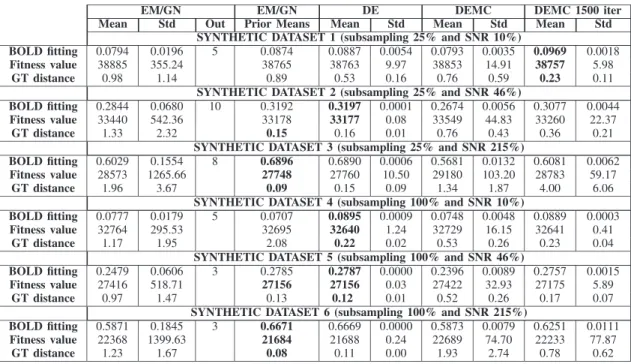
TABLE II
DE, EM/GNANDDEMC OPTIMIZATIONVALUES FOREACH OF THE6 SYNTHETICDATASETS. THEDECIMALSHAVEBEENREMOVED IN THEMEANFITNESSVALUES TOFACILITATEVISUALIZATION ANDCOMPARISONBETWEENMETHODS. THEBESTRESULTSOBTAINED
PERDATASET AREDISPLAYED INBOLD. THELOWER THEFITNESSVALUE THEBETTER THERESULT
the two stochastic approaches. Also, in order to study its gen-eral behavior, EM/GN [9] was executed 100 times from random initializations (including the prior means). Finally, DEMC was also run using 1500 iterations in order to verify the improve-ment in performance associated with a larger execution time. All methods are implemented in MATLAB and the total number of runs was 2700, corresponding to 1800 optimization runs with real data (12 rats, 100 repetitions of EM/GN, 20 repetitions of DE and DEMC, and 10 repetitions using DEMC with 1500 itera-tions) and 900 optimization runs with synthetic data (6 synthetic datasets, 100 repetitions of EM/GN, 20 repetitions of DE and DEMC, and 10 repetitions using DEMC with 1500 iterations). Each EM/GN iteration implies 21 integrations of the differen-tial equations (the most time consuming task within the fitness function), while in DE and DEMC each iteration needs 150 in-tegrations (45000 integration operations per run).
The main idea behind the convergence criteria in DE is that there is a minimum fitness value to reach ( , in this case 0), and the optimization algorithm will stop its minimization of function if either the maximum number of iterations
(in this case 300) is reached, like in DEMC, or the best param-eter vector has found a value .
To trigger further research in the estimation of biophysical parameters using neuroscientific models, our synthetic datasets and the toolbox implementing the proposed approach will be made publicly available at HAL repository.
C. Synthetic Data Results
The three metrics used to evaluate performance were the BOLD fitting measure (to be maximized), the fitness value (to be minimized) and the distance to GT (to be minimized). The BOLD fitting measure, computed as where is the variance of the raw data and is the variance of
the residuals after fitting the model, represents the amount of variance in the original signal which is explained by the model: the value is 1 if the fitting is perfect and smaller than 0 if the final set of parameters found is fitting the actual signal worse than a zero BOLD signal. In turn, the fitness value corresponds to the value achieved by the optimization methods according to (4), and the GT distance for a particular parameter set is de-termined by the root mean square of , where is the GT and represents the estimated parameter set found respec-tively by each optimization algorithm. Importantly, to compute the GT distance only physiologically meaningful parameters (last seven parameters in Table I: from to ) are taken into account. Since EM/GN is very dependent on the initialization and may perform poorly if the initial configuration is far from a global optimum, we perform an outlier rejection procedure prior to calculating the average performance consisting simply on the removal of solutions which provide a negative or zero BOLD fitting value.
The mean number of EM/GN iterations to converge was 37 18 (max: 135, min: 11), so the average number of integrations to obtain the final result is 784. Table II contains the mean and standard deviation of the results obtained by each method and synthetic dataset. Column 4 indicates the number of results not taken into account to compute the statistics. We have also in-cluded a column with the solution found running EM/GN using the prior means as initial values. The last two columns show the results obtained by DEMC using 1500 iterations to verify the improvement achieved by increasing the execution time. Fig. 1 displays the distributions of the parameter estimates found for four physiologic parameters.
Among the methods under comparison, DE shows the most stable behavior, achieving a similar performance in different runs. This is confirmed both by the low standard deviation of
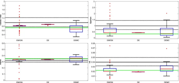
Fig. 1. Boxplots for parameters for synthetic dataset 2. The green horizontal line represents the GT and the diamond displays the estimate achieved using EM/GN from the prior means. Since the actual EM/GN spread is much larger in all cases, we have zoomed-in on a sub-interval to better visualize the differences between the methods. The prior means and prior covariances are displayed as horizontal solid and dashed black lines, respectively.
Fig. 2. Boxplots of the EM/GN, DE and DEMC results for , , transit time , and using globally all real datasets. The parameters prior mean and standard deviation are indicated by the horizontal black lines (solid and dashed, respectively). Since the EM/GN variability is much larger in all cases, we have zoomed-in on a sub-interval for a better visualization.
the fit quality metrics as well as the reduced variability in pa-rameter space. EM/GN on the other hand appears to be very dependent on the initialization and generally shows the highest spread in all metrics. Also, DE presents on average the best per-formance according to the three metrics under consideration. The improvement obtained by DEMC when running 1500
it-erations (with respect to using 300 itit-erations) could justify the increase in computational time. Within each dataset, both the BOLD fitting measure as well as the fitness value are consis-tently correlated with the GT distance, providing evidence that these first two measures are good markers of the quality of the parameter estimates found.
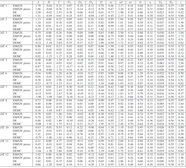
TABLE III
DE, EM/GNANDDEMC MEDIANESTIMATES FOREACH OF THE12 RATS ANDEACHPARAMETER IN . FORDEANDDEMCTHEVALUESCORRESPOND TO THEMEDIAN OF20 VALUES. FOREM/GNTHEVALUESCORRESPOND TO THEMEDIAN OF100 VALUES
Surprisingly, in Table II, for synthetic dataset 3, increasing the number of iterations up to 1500 in DEMC degrades the results in terms of mean GT distance and standard deviation. A plau-sible explanation for this phenomenon could be found in the ex-ploratory nature of DEMC and the characteristics of the problem at hand. It seems like DEMC intensively explores the search space and it is able to find very diverse solutions which are better in terms of BOLD fitting and fitness value. But, those sets of parameters are progressively different from the GT. On the other hand, this possible explanation would go in the same di-rection that other research works [34], [36], where very different parameters could give nearly identical BOLD output; meaning that, without properly constraining the parameter values, some of them may not be precisely ascertainable. This could explain discrepancies of parameter estimates in previous studies.
Fig. 1 shows that, for all four parameters considered here, the average estimates tend to be generally closer to the GT than to the prior means. This indicates that these particular model parameters can be identified from BOLD data.
D. Real Data Results
In EM/GN, the average number of iterations until conver-gence is 31 18 (max: 128, min: 8) with an average number of integrations of 646. The median estimates from DE, DEMC and EM/GN are shown in Table III. The experimental condi-tions for all animals were controlled as closely as possible. It is therefore expected that the physiologically meaningful param-eters show limited variability across animals. However, the pa-rameters related to the scaling of the stimulus (notably, , and ) may vary significantly, since the amplitudes of the elicited
Fig. 3. Median fitness evolution for each optimization method in rats 1 (left) and 10 (right), respectively. We have zoomed-in on a sub-interval to get the nuances of the error evolution.
EEG responses varied between sessions. Even though the ad-ministration protocol was performed to be identical to the extent possible, the amount of the drug that actually ended up in the tissue likely varied between animals depending on factors such as the diffusion or leakage of the drug along the injection path. The injected drug, bicuculline methochloride, is an antagonist of receptors, and thus modulates the coupling from in-hibitory to excitatory neurons, represented by the parameters , and . We observe significant variability in these parameters, both across animals and across optimization methods. Analysis of this variability is complicated by the fact that , and interact and variations in one of the parameters may be partially compensated by variations in another. Thus, the observed vari-ability may also be due to identifivari-ability issues. Estimates across animals for four of the parameters that are expected to be among the most stable, namely , , and , are shown in Fig. 2.
The estimates found by DEMC for are less stable and re-markably lower than the ones found by EM/GN and DE. This behavior can possibly be explained using the same arguments used for synthetic dataset 3 in Table II (DEMC exploratory ability and identifiability issues), and also considering that the values found for , due to the complexity of the problem, can balance out with the values found for other parameters in a way that can equally result in a good fitness value.
Fig. 3 shows the median fitness evolution for two different cases (rats 1 and 10, respectively), and also highlights that DE and DEMC are able to continue exploring the search space, im-proving the solutions found, while EM/GN is prone to converge to a local optimum. According to this figure, a smaller number of DE iterations might have been sufficient to achieve a good result: the x-axis of Fig. 3 uses a logarithmic scale and, from it-erations 150 to 300, the improvement achieved by DE is almost irrelevant compared to the doubling in computation time neces-sary for the extra 150 iterations.
The values estimated by DE are markedly more stable than the values obtained with EM/GN and DEMC. Quantitatively, the median parameter estimates from all three methods are plau-sible. Blood transit times from arterioles to the deoxygenated vascular compartment estimated with all methods are closer to 0.7 s which is somewhat lower than the prior mean of 0.98 s but still physiologically plausible. Individual runs of EM/GN
Fig. 4. Compact boxplots for and transit time per rat and algorithm. EM/GN, DE and DEMC are displayed using red, blue and green lines, respec-tively. The median values for each optimizer are linked by colored dashed lines. We have zoomed-in on the sub-interval because the actual EM/GN spread is much larger in all cases. The prior mean and covariance are indicated by the horizontal black lines (solid and dashed, respectively).
can lead to much lower or higher unphysiologic estimates, de-pending on the initial value used in the estimation (Fig. 4 and Table III). For comparison, mean transit times across the entire vascular tree in a cortical voxel observed using DSC MRI in anesthetized rats are on the order of 1.6 s (from [37]). Equally, estimated resting venous blood volumes are lower than the prior estimate of 4% taken from SPM defaults, which also corre-sponds to the total cortical resting blood volume in isoflurane anesthetized male Wistar rats [37]. In hindsight, the value that should actually be considered in the model is however only the venous (deoxygenated) fraction of that, such that a value of 2% actually seems much more realistic than the much higher values estimated in some of the runs using EM/GN and DEMC. Finally,
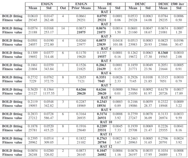
TABLE IV
OPTIMIZATIONVALUES FOREACH OF THE12 RATS. THEDECIMALSHAVEBEENREMOVED IN THEMEANFITNESSVALUES. THEBESTRESULTS
OBTAINED PERRAT AREDISPLAYED INBOLD. THELOWER THEFITNESSVALUE THEBETTER THERESULT
all methods on average yield values for the intra- to extra-vas-cular BOLD signal ratio and Grubb exponent that are similar across methods. Estimates are close to the prior means for the Grubb exponent. Given the results obtained on synthetic data, this is an indication that the prior means are close to the un-known GT. In summary, the estimates obtained from DE for these values seem both more stable and more realistic or at least as realistic across sessions as the estimates from EM/GN and DEMC. Fig. 4 displays the boxplots per method and rat for and where DE presents again a very low variability. It is im-portant to highlight that EM/GN without at least several runs with different initial values produces unstable results (both in terms of the fitness function value, as witnessed by their large standard deviation, as well as in parameter values, as shown in the boxplots), but other methods, like DE, can solve this problem in a stable fashion, given prior information.
The fitness values achieved per method (mean and standard deviation) are shown in Table IV using the same criteria as ex-plained in Section V-C. DE again is the best method in terms of BOLD fitting and fitness value. It is important to emphasize the different nature of the algorithms under study: EM/GN works with only one solution in a deterministic fashion, while DE and
DEMC deal with a population of candidate solutions with a sto-chastic strategy. Commonly, DE and DEMC (especially when using 1500 iterations) have a more stable behavior as reflected in a lower standard deviation. These results can have a deci-sive impact within the neuroscientific community since, from the practical point of view, neuroscientists usually select one single starting solution and run EM/GN from there, obtaining sometimes reasonable results but, also quite commonly, clearly improvable ones (in Table IV, the results obtained by DE out-performed the ones obtained by EM/GN from the prior means, i.e. our best estimate of parameter values based on existing lit-erature).
Statistical tests were performed to study the statistical sig-nificance of the results obtained in terms of BOLD fitting and fitness value (see Table V): the mean ranks represent the av-erage position of each method per rat, while the p-value is com-puted using a non-parametric statistical test (since the normality and homoscedasticity assumptions are not met, as usual with EC methods [38]) between the first method and the other two. As shown in Table V, DE and DEMC, in real data, are on average the first and the second best methods according to both fitness function value and BOLD fitting.
TABLE V
OVERALLAVERAGERANKACHIEVED BYEACHOPTIMIZATIONMETHOD ANDADJUSTED P-VALUE OFWILCOXONRANKSUMTESTCOMPARINGEACH
ALGORITHMAGAINST THERANKEDFIRSTONE INREALDATA
VI. CONCLUSION ANDFUTUREWORK
Two stochastic methods (DE and DEMC) have been applied to estimate biophysical parameters in fMRI data and they have proven to be able to obtain physiologically feasible results. In particular, DE shows the robustness and flexibility of global search optimization methods while being able to incorporate prior information in a principled Bayesian way. DEMC can also provide consistent solutions but with a much larger number of iterations. Preliminary results on real and synthetic data show that DE is able to achieve sensible parameter estimates with a more stable and consistent behavior, improving in terms of fitness value and fMRI signal fitting in real data, than the tra-ditional and widely used EM/GN approach (de facto standard in the SPM package). Traditionally in cognitive neuroscience EM/GN is run from the prior means to obtain the estimates, but the large spread in parameter values and its lack of reliability in terms of fitness values provide evidence to justify the use of stochastic approaches (either EM/GN from different random initial solutions or a MH-based approach). The formulation pre-sented here is generic and can be adapted to other forward gen-erative models that relate neuronal and physiological variables to macroscopic data (e.g. [39]–[41]), mainly by modifying func-tions and (Section III).
Before issuing a definitive conclusion, DE should be com-pared with alternative approaches like single-chain adaptive MCMC [42], Hamiltonian MCMC [43], Belief Propagation [44] or Langevin diffusion [45]. Also, as future work, we could take advantage of the inherent property of EC methods to provide a set of solutions instead of a single one, giving information about the range of values for each parameter that are consistent with the data. Testing on multimodal fMRI data may also help to further improve the reliability of the parameter estimates, since cerebral blood flow and volume dynamics can provide additional information.
ACKNOWLEDGMENT
The authors thank J.-F. Scariot and T. Perret for their ex-tremely valuable help regarding the technical tools used.
REFERENCES
[1] R. B. Buxton, E. C. Wong, and L. R. Frank, “Dynamics of blood flow and oxygenation changes during brain activation: The balloon model,”
Magn. Reson. Med., vol. 39, pp. 855–864, 1998.
[2] R. B. Buxton, K. Uludağ, D. J. Dubowitz, and T. T. Liu, “Modeling the hemodynamic response to brain activation,” NeuroImage, vol. 23, pp. S220–S233, 2004.
[3] K. J. Friston, A. Mechelli, R. Turner, and C. J. Price, “Nonlinear re-sponses in fMRI: The balloon model, Volterra kernels, and other hemo-dynamics,” NeuroImage, vol. 12, pp. 466–477, Jun. 2000.
[4] I. Khalidov, J. Fadili, F. Lazeyras, D. Van De Ville, and M. Unser, “Activelets: Wavelets for sparse representation of hemodynamic re-sponses,” Signal Process., vol. 91, no. 12, pp. 2810–2821, 2011. [5] A. Frau-Pascual, P. Ciuciu, and F. Forbes, “Physiological models
com-parison for the analysis of ASL fMRI data,” in Proc. 12th IEEE Int.
Symp. Biomed. Imag. (ISBI), 2015, pp. 1348–1351.
[6] A. Frau-Pascual, T. Vincent, J. Sloboda, P. Ciuciu, and F. Forbes, “Physiologically informed Bayesian analysis of ASL fMRI data,” in
Proc. 1st Int. Workshop Bayesian grAphical Models for Biomed. Imag. (BAMBI), 2014, vol. 8677, ser. LNCS, pp. 37–48.
[7] K. E. Stephan, N. Weiskopf, P. M. Drysdale, P. A. Robinson, and K. J. Friston, “Comparing hemodynamic models with DCM,” NeuroImage, vol. 38, no. 3, pp. 387–401, 2007.
[8] O. David, I. Guillemain, S. Saillet, S. Reyt, C. Deransart, C. Segebarth, and A. Depaulis, “Identifying neural drivers with functional MRI: An electrophysiological validation,” PLoS Biol., vol. 6, no. 12, pp. 2683–2697, 2008.
[9] K. J. Friston, “Bayesian estimation of dynamical systems: An applica-tion to fMRI,” NeuroImage, vol. 16, no. 2, pp. 513–530, 2002. [10] , K. Friston, J. Ashburner, S. Kiebel, T. Nichols, and W. Penny, Eds.,
Statistical Parametric Mapping: The Analysis of Functional Brain Im-ages. New York, NY, USA: Academic, 2007.
[11] P. Mesejo, A. Valsecchi, L. Marrakchi-Kacem, S. Cagnoni, and S. Damas, “Biomedical image segmentation using geometric deformable models and metaheuristics,” Comput. Med. Imag. Grap., vol. 43, pp. 167–178, 2015.
[12] C. Svensson, S. Coombes, and J. W. Peirce, “Using evolutionary algo-rithms for fitting high-dimensional models to neuronal data,”
Neuroin-formatics, vol. 10, no. 2, pp. 199–218, 2012.
[13] M.-H. Kao, A. Mandal, N. A. Lazar, and J. Stufken, “Multi-objective optimal experimental designs for event-related fMRI studies,”
Neu-roImage, vol. 44, no. 3, pp. 849–856, 2009.
[14] T. Wager and T. Nichols, “Optimization of experimental design in fMRI: A general framework using a genetic algorithm,” NeuroImage, vol. 18, no. 2, pp. 293–209, 2003.
[15] B. Maus, G. J. P. V. Breukelen, R. Goebel, and M. P. F. Berger, “Ro-bustness of optimal design of fMRI experiments with application of a genetic algorithm,” NeuroImage, vol. 49, no. 3, pp. 2433–2443, 2010. [16] M. Pyka, D. Heider, S. Hauke, T. Kircher, and A. Jansen, “Dynamic causal modeling with genetic algorithms,” J. Neurosci. Meth., vol. 194, no. 2, pp. 402–406, 2011.
[17] J. R. Chumbley, K. J. Friston, T. Fearn, and S. J. Kiebel, “A Metropolis-Hastings algorithm for dynamic causal models,” NeuroImage, vol. 38, no. 3, pp. 478–487, 2007.
[18] V. A. Vakorin, O. O. Krakovska, R. Borowsky, and G. E. Sarty, “In-ferring neural activity from BOLD signals through nonlinear optimiza-tion,” NeuroImage, vol. 38, no. 2, pp. 248–260, 2007.
[19] A. Marreiros, S. Kiebel, and K. Friston, “Dynamic causal modelling for fMRI: A two-state model,” NeuroImage, vol. 39, no. 1, pp. 269–278, 2008.
[20] M. Silvennoinen, C. Clingman, X. Golay, R. Kauppinen, and P. van Zijl, “Comparison of the dependence of blood R2 and on oxygen saturation at 1.5 and 4.7 Tesla,” Magn. Reson. Med., vol. 49, no. 1, pp. 47–60, 2003.
[21] K. Stephan, L. Kasper, L. Harrison, J. Daunizeau, H. den Ouden, M. Breakspear, and K. Friston, “Nonlinear dynamic causal models for fMRI,” NeuroImage, vol. 42, no. 2, pp. 649–662, 2008.
[22] M. Kobayashi, T. Mori, Y. Kiyono, V. Tiwari, R. Maruyama, K. Kawai, and H. Okazawa, “Cerebral oxygen metabolism of rats using injectable (15)o-oxygen with a steady-state method,” J. Cereb. Blood
Flow Metab., vol. 32, no. 1, pp. 33–40, 2012.
[23] T. Watabe, E. Shimosegawa, H. Watabe, Y. Kanai, K. Hanaoka, T. Ueguchi, K. Isohashi, H. Kato, M. Tatsumi, and J. Hatazawa, “Quan-titative evaluation of cerebral blood flow and oxygen metabolism in normal anesthetized rats: 15O-labeled gas inhalation PET with MRI Fusion,” J. Nucl. Med., vol. 54, no. 2, pp. 283–290, 2013.
[24] A. Gelman, J. B. Carlin, H. S. Stern, and D. B. Rubin, Bayesian Data
Analysis, 2nd ed. Boca Raton, FL, USA: Chapman and Hall/CRC,
2003, Chapman & Hall/CRC Texts in Statistical Science.
[25] A. E. Eiben and J. E. Smith, Introduction to Evolutionary
Com-puting. Berlin, Germany: Springer-Verlag, 2003.
[26] M. D. Vose, The Simple Genetic Algorithm: Foundations and
Theory. Cambridge, MA, USA: MIT Press, 1998.
[27] W. Gutjahr, “Convergence analysis of metaheuristics,” in
Metaheuris-tics, ser. Annals of Information Systems. New York, NY, USA:
[28] X.-S. Yang, “Metaheuristic optimization: Algorithm analysis and open problems,” in , P. M. Pardalos, Ed., S. Rebennack, Ed. New York, NY, USA: Springer, 2011, pp. 21–32.
[29] S. Das and P. Suganthan, “Differential evolution: A survey of the state-of-the-art,” IEEE Trans. Evolut. Comput., vol. 15, no. 1, pp. 4–31, 2011.
[30] P. Mesejo, R. Ugolotti, F. D. Cunto, M. Giacobini, and S. Cagnoni, “Automatic hippocampus localization in histological images using dif-ferential evolution-based deformable models,” Pattern Recog. Lett., vol. 34, no. 3, pp. 299–307, 2013.
[31] Y. S. Nashed, P. Mesejo, R. Ugolotti, J. Dubois-Lacoste, and S. Cagnoni, “A comparative study of three GPU-based metaheuristics,” in Parallel Problem Solving From Nature (PPSN), 2012, vol. 7492, ser. LNCS, pp. 398–407.
[32] C. J. F. ter Braak, “A Markov chain Monte Carlo version of the genetic algorithm differential evolution: Easy Bayesian computing for real pa-rameter spaces,” Statist. Comput., vol. 16, no. 3, pp. 239–249, 2006. [33] K. Friston, J. Mattout, N. Trujillo-Bareto, J. Ashburner, and W. Penny,
“Variational free energy and the Laplace approximation,” NeuroImage, vol. 34, no. 1, pp. 220–234, 2007.
[34] M. C. Chambers, “Full brain blood-oxygen-level-dependent signal pa-rameter estimation using particle filters,” M.S. thesis, Virginia Poly-technic Inst. and State Univ., Blacksburg, VA, USA, 2010.
[35] S. Makni, P. Ciuciu, J. Idier, and J.-B. Poline, “Joint detection-estima-tion of brain activity in fMRI using an autoregressive noise model,” in
Proc. 3rd IEEE Int. Symp. Biomed. Imag. (ISBI), 2006, pp. 1048–1051.
[36] T. Deneux and O. Faugeras, “Using nonlinear models in fMRI data analysis: Model selection and activation detection,” NeuroImage, vol. 32, no. 4, pp. 1669–1689, 2006.
[37] N. Coquery, O. Francois, B. Lemasson, C. Debacker, R. Farion, C. Rémy, and E. L. Barbier, “Microvascular MRI and unsupervised clustering yields histology-resembling images in two rat models of glioma,” J. Cereb. Blood Flow Metab., vol. 34, no. 8, pp. 1354–1362, 2014.
[38] J. Derrac, S. García, D. Molina, and F. Herrera, “A practical tutorial on the use of nonparametric statistical tests as a methodology for com-paring evolutionary and swarm intelligence algorithms,” Swarm Evol.
Comput., vol. 1, no. 1, pp. 3–18, 2011.
[39] A. L. Vazquez, E. R. Cohen, V. Gulani, L. Hernandez-Garcia, Y. Zheng, G. R. Lee, S.-G. Kim, J. B. Grotberg, and D. C. Noll, “Vascular dynamics and BOLD fMRI: CBF level effects and analysis considera-tions,” NeuroImage, vol. 32, no. 4, pp. 1642–1655, Oct. 2006. [40] P. A. Valdes-Sosa, J. M. Sanchez-Bornot, R. C. Sotero, Y.
Iturria-Medina, Y. Aleman-Gomez, J. Bosch-Bayard, F. Carbonell, and T. Ozaki, “Model driven EEG/fMRI fusion of brain oscillations,” Human
Brain Map., vol. 30, no. 9, pp. 2701–2721, 2009.
[41] M. Havlicek, A. Roebroeck, K. Friston, A. Gardumi, D. Ivanov, and K. Uludag, “Physiologically informed dynamic causal modeling of fMRI data,” NeuroImage, vol. 122, pp. 355–372, 2015.
[42] B. Sengupta, K. J. Friston, and W. D. Penny, “Gradient-free MCMC methods for dynamic causal modelling,” NeuroImage, vol. 112, pp. 375–381, 2015.
[43] B. Sengupta, K. J. Friston, and W. D. Penny, “Gradient-based MCMC samplers for dynamic causal modelling,” NeuroImage, 2015, to be pub-lished.
[44] D. Baron, S. Sarvotham, and R. Baraniuk, “Bayesian compressive sensing via belief propagation,” IEEE Trans Signal Process., vol. 58, no. 1, pp. 269–280, Jan. 2010.
[45] G. Roberts and O. Stramer, “Langevin diffusions and Metropolis-Hast-ings algorithms,” Methodol. Comput. Appl. Probab., vol. 4, no. 4, pp. 337–357, 2002.
Pablo Mesejo received the M.Sc. and Ph.D. degrees
in computer science from Universidade da Coruña (Spain) and Università degli Studi di Parma (Italy), respectively. He performed his Ph.D. as Early Stage Researcher within the Marie Curie ITN MIBISOC (“Medical Imaging using Bio-Inspired and SOft Computing”). After that, he was working as Post-doctoral Researcher at the ALCoV team (Advanced Laparoscopy and Computer Vision) of Université d'Auvergne (France). Currently he is a Postdoctoral Researcher for INRIA Grenoble Rhône-Alpes (France). His research interests include computer vision and bio-inspired/soft computing methods, as well as their application to real-world problems in biomedical image/signal processing and analysis.
Sandrine Saillet graduated in Biologie Intégrative
et Physiologie from Université Pierre et Marie Curie, Paris, France, in 2006 and Ph.D. degree in Neuro-science from Université Joseph Fourier, Grenoble, France, in 2010. After that, she was a Postdoctoral Researcher at the Institut de Neurosciences des Systèmes, Marseille, France and at Grenoble Institut des Neurosciences, Grenoble, France, respectively. Since 2014, she is a Postdoctoral Researcher at the Gladstone Institutes, San Francisco, United States of America. Her expertise is in electrophysiology and her main research area is currently focused on understanding the neuronal processes underlying cognitive decline in Alzheimer's disease.
Olivier David graduated in applied physics from
Ecole Normale Supérieure in 1999 and is an expert of functional neuroimaging, electrophysiology and neural modeling. In 2005, he obtained a tenure position to coordinate an EEG/fMRI program in humans and rodents at the Inserm U836 Grenoble Institute of Neuroscience, France. The main focus of his current research is to understand the effects of brain electrical stimulation on the organization of functional networks using fMRI, intracerebral EEG and neural modeling.
Christian G. Bénar (M’99–SM’15) was born in
Dijon (France) in 1971. He received the engineering degree from Ecole Supélec (Metz and Paris, France) in 1994, and the Ph.D. degree in biomedical engi-neering from McGill University (Montréal, Canada) in 2004. He worked for Stellate Systems (Montréal) on software for EEG analysis between 1995 and 1997. Since 2006 he has been a Researcher at INSERM in Marseille (France). In 2012 he became head of the Dynamical Brain Mapping team at Institut de Neurosciences des Systèmes (INS), a joint INSERM-Aix-Marseille University laboratory. Since 2015 he has been the scientific head of the Magnetoencephalography (MEG) platform of the INS, hosted in the clinical neurophysiology department of the Timone hospital from AP-HM in Marseille. His main area of research is multimodal signal processing for brain mapping, in particular EEG, MEG and intracerebral EEG, with application to cognition and epilepsy.
Jan M. Warnking received masters degrees in
physics from the State University of New York at Stony Brook, US, and from the Julius Maximilians Universität Würzburg, Germany, and a Ph.D. in physics from the Universitè Joseph Fourier in Grenoble, France. Since 2007 he has held a tenure position at the Institut National pour la Santé et la Recherche Médicale (Inserm) working at the Grenoble Institute of Neuroscience. His expertise is in MR physics and his research activities cover work on human and small animal fMRI data acquisition and biophysical models, cerebral blood flow and vasoreactivity measurements, as well as MR safety of implants.
Florence Forbes received the B.Sc. and M.Sc.
de-grees in computer science and applied mathematics from the Ecole Nationale Supérieure d'Informa-tique et Mathémad'Informa-tiques Appliquées de Grenoble (ENSIMAG), France, and the Ph.D. degree in applied probabilities from the University Joseph Fourier, Grenoble, France. Since 1998, she has been a Research Scientist with the Institut National de Recherche en Informatique et Automatique (INRIA), Grenoble Rhône-Alpes, Montbonnot, France, where she founded the MISTIS team and has been the team head since 2003. Her research activities include Bayesian analysis, Markov and graphical models, and hidden structure models.