Fast computation and applications of genome mappability.

(1)

Fast Computation and Applications of Genome

Mappability

Thomas Derrien1*, Jordi Estelle´2, Santiago Marco Sola2, David G. Knowles3, Emanuele Raineri2, Roderic Guigo´3, Paolo Ribeca2*

1 Institut de Ge´ne´tique et De´veloppement (IGDR), Universite´ Rennes 1, Rennes, France, 2 Centro Nacional de Ana´lisis Geno´mico (CNAG), Barcelona, Spain, 3 Centre for Genomic Regulation (CRG), Universitat Pompeu Fabra, Barcelona, Spain

Abstract

We present a fast mapping-based algorithm to compute the mappability of each region of a reference genome up to a specified number of mismatches. Knowing the mappability of a genome is crucial for the interpretation of massively parallel sequencing experiments. We investigate the properties of the mappability of eukaryotic DNA/RNA both as a whole and at the level of the gene family, providing for various organisms tracks which allow the mappability information to be visually explored. In addition, we show that mappability varies greatly between species and gene classes. Finally, we suggest several practical applications where mappability can be used to refine the analysis of high-throughput sequencing data (SNP calling, gene expression quantification and paired-end experiments). This work highlights mappability as an important concept which deserves to be taken into full account, in particular when massively parallel sequencing technologies are employed. The GEM mappability program belongs to the GEM (GEnome Multitool) suite of programs, which can be freely downloaded for any use from its website (http://gemlibrary.sourceforge.net).

Citation: Derrien T, Estelle´ J, Marco Sola S, Knowles DG, Raineri E, et al. (2012) Fast Computation and Applications of Genome Mappability. PLoS ONE 7(1): e30377. doi:10.1371/journal.pone.0030377

Editor: Christos A. Ouzounis, The Centre for Research and Technology Hellas, Greece Received January 28, 2011; Accepted December 19, 2011; Published January 19, 2012 Copyright: ß

(2)

studies the mappability of various genomes has been investigated without considering mismatches. However, one must make provision for sequencing errors inherent to HTS technologies, as well as for polymorphisms or variants between the individual genome/transcriptome actually sequenced and the genome used as a mapping reference. Therefore, it is customary to allow for mismatches when mapping reads; the 0-mismatch mappability is not sufficient in these cases. Unfortunately, computing the mappability of a sequence up to even a few mismatches is usually a task orders of magnitude more expensive than when no mismatches are allowed, and hence not one routinely performed. In this work, we introduce and describe a mapping-based method to compute the mappability of an entire sequence of the size of a mammalian genome up to an arbitrary number of mismatches, which is guaranteed to be comparatively fast even for short reads and very redundant sequences. The method produces the exact mappability in the case of 0 mismatches, and a very good approximation of it if a non-zero number of mismatches is allowed. For different number of substitutions, we then examine the genome-wide mappability profiles of four model organisms (human, mouse, fly and nematode), for which we also produced visualization schemes as part of the UCSC genome browser [7].

Second, we study the mappability of the transcribed genomic regions. Since a high proportion of transcripts in a genome exhibit repetitive sequences –such as repeated functional units or retro-transposons (LINEs and SINEs)– which can influence their mappability profiles, we use our mappability method to explore the variations in mappability of different classes of transcripts, taking the GENCODE annotation [8] as a reference. We show that indeed mappability profiles vary greatly with the transcript class (protein-coding genes, non coding RNAs, orthologous families, etc). We thus propose an improved measure of RNA quantification which takes into account the mappability at the level of the single locus.

Third, we investigate how the use of paired-end sequencing or mate-pair libraries relates to mappability. To this end, we predict and quantify how many of the pairs obtained from a typical DNASeq experiment can be rescued by taking advantage of the uniqueness of one of its reads and of the distance information for the pair.

In conclusion, we are able to precisely link our findings to the design of a better experiment when the focus is on some particular element in the genome. Our results suggest that the mappability is an important concept to be taken into account when one is trying, for instance, to re-sequence a particular genomic region, or to produce quantitative estimates of transcript abundance from RNASeq experiments.

Methods

Formally, our definition of the mappability is the following. Given some read length k, the k-frequency Fk(x) of a sequence at a given position x corresponds to the number of times the k-mer starting at position x appears in the sequence and in its reverse complement, considering as equivalent all the k-mers which differ by less than some predefined alignment score (like a given number of mismatches–for the sake of simplicity, in the rest of this paper we will assume a framework where only substitutions, and neither insertions nor deletions, are allowed during alignment). For instance, the 2-frequency up to 1 substitution of the string TICTACTOE at positions 1 to 8 is given by the values 3,2,2,3,2,2,3,1. It is possible to define an analogous quantity, the k-mappability or k-uniqueness Mk(x), as the inverse of the frequency: Mk(x)~1=Fk(x). While the frequency usually varies by several

orders of magnitude, the mappability has the advantage of always being a quantity between 0 and 1, and such that the highest possible values of 1 correspond to uniquely mapping position (here, and throughout all the paper, by ‘‘unique’’ we mean ‘‘unique up to the specified number of mismatches’’).

Various methods can be employed to compute the exact frequency (and hence the mappability) of a sequence. The simplest one is a brute-force approach, consisting in the explicit enumeration and counting of all the k-mers present in the sequence; it is practical only for very short strings. More sophisticated strategies might rely on the traversal of some string data structure –like a suffix tree, a suffix array or a hash table– to directly obtain an enumeration of the k-mers together with their counts; this is what has been used in [5,6]. All such approaches, however, become problematic if mismatches are allowed: the authors of [6] report for their method a slowdown of a factor of 400 when 2 substitutions are permitted, and they do not go further than evaluating the mappability of just 1 Mb of the human genome using such an edit distance.

In the case of mismatches, essentially, the problem of computing the frequencies becomes equivalent to that of exhaustively mapping all the positions in the sequence after a suitable choice of the alignment parameters. At a first glance, this goal would seem well within the range of existing high-performance mappers, which may easily attain speeds of several tens of millions of mapped reads per hour; assuming a mapping speed of 107_reads per hour, for instance, it would appear possible to compute the frequencies of the human genome in only about 300 hours, with the additional possibility of distributing the computation among different processors.

There are two algorithmic issues, however. The first one is that most of the available mappers are not based on exhaustive alignment algorithms; this fact implies that they are unable to report the exact count of all the existing matches for a given sequence (although they can usually return a more or less precise approximation of such a quantity). The second problem concerns performance: most mapping algorithms are usually optimized to quickly report a few matches and most of them become (much) slower when requested to perform full counting queries. In practice, the speed of all implementations of mapping algorithms always shows some dependency on the number of matches found in the reference; this means that aligning one million reads which all map to thousands of locations in the genome will be (much) slower than aligning one million reads mapping uniquely. Performance degradation may become very relevant in the case of a brute-force enumeration of a sequence in a genome (for instance, it is still possible to find in H.sapiens genomic locations having 50-mappability as large as 10,000 when 2 substitutions are allowed – like ACGGTGGCTCATGCCTGTAATCCCAGC-ACTTTGGGAGGCCGAGGCGGGCG, which appears 15,323 times with less than 3 nucleotide substitutions). In general, performance will be worse when the mappability of a transcrip-tome is being evaluated, and dramatically worse when small values for k are used, as in typical ChIPSeq or MNaseSeq experiments. In our framework, the first problem is automatically taken care of by our own genome indexing implementation, which provides for fast exhaustive searches and counting queries [2]. We address the second issue by noting that most of the degradation in performance actually comes from the fraction of k-mers showing high frequencies, where thousands of k-mers exist which are equivalent within the specified number of mismatches; thus, most of the computational time is actually spent mapping such set of k-mers over and over again, each time any single element of the set is mapped.

Fast Computation of Genome Mappability

(3)

To avoid the latter problem at least in part, we perform the following approximation: each time a k-mer is mapped within the given number of mismatches to a set of positions S, one can pretend that all the positions in S have already been mapped, assign to them a frequency value equal to the number of elements inS, and skip them altogether from that point on. Such a strategy is not enough to completely factor the redundancy out –it is effective in eliminating only the equivalent k-mers occurring in the sequence after the mer being mapped–, and is only exact for k-frequencies when no substitutions are allowed. From a practical standpoint, however, the mappability computed in this way is a good approximation of the exact mappability, and, more importantly, is computationally feasible even when k is small. The complete algorithm is as follows.

Algorithm 1 (Fast mappability computation) To compute the k-frequencies of a sequence of length n up to m mismatches, given an approximation parameter tw0:

1.initialize and zero an array F of n numbers 2.for all positions i in the sequence do

if F ið Þ~0 then

(a) take the k-mer S starting at position i

(b) compute all the positionsP in the sequence to which S maps up to m mismatches

(c)set F ið Þ : ~cardinality Pð Þ (d)if cardinalityð Þwt thenP for all positions j inP do if F jð Þ~0 then

set F jð Þ : ~cardinality Pð Þ else

set F jð Þ : ~ max cardinality Pð ð Þ,F jð ÞÞ 3.output the array F .

When mw0, the proposed algorithm provides approximated values for the frequency of positions which are not unique in the sequence: this is due to the fact that, given two different k-mers K1 and K2, the setSK1 of locations equivalent to K1up to the given

number of mismatches is in general different from the set of locations SK2 equivalent to K2; hence, considering

cardinalityðSK1Þ as the frequency of both K1 and K2 is an

approximation. However, as stated above the algorithm is acceptable from a practical standpoint since:

1. it is exact for the whole sequence when m~0

2. when mw0 it still gives correct values for the frequency of the k-mers that are unique within the specified number of mismatches, as a k-mer Ki can belong to the set SKj of

locations equivalent to a previously occurring k-mer Kjonly if it is not unique; in addition, the parameter t allows to propagate an approximated frequency value only when it is sufficiently large

3. the difference between approximated and real frequency can be large in absolute terms, but in the majority of cases it represents only a relatively small fraction of the correct value, since the optimization affects the locations in proportion to their redundancy.

Another important observation is about the presence of the maximum function in the else branch of case (2d): this choice regulates the case when a k-mer is hit more than once during the mapping of other similar k-mers. Since the frequency of the k-mer will not be directly recomputed due to the chosen optimization strategy, the maximum of all the possibilities is taken as its value, to

make sure that an underestimation of the actual value is avoided as much as possible.

Finally, we emphasize that when the exact mappability is needed the approximation can always be turned off by setting t~?: this produces exact frequencies, albeit at the price of possibly much longer running times if k is small and/or the genome is very repetitive.

We made use of the latter property to test our approximation, and assess how well it correlates with the exact results. To this end we performed two runs for each example, one with the value of t automatically selected by the program, and another with t~?; we then compared the results thus obtained.

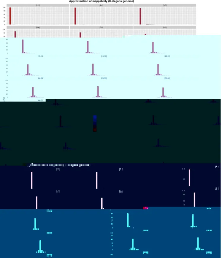
We applied such a procedure to both the complete genome of C.elegans (using the default value of t~6 versus ?, see Figure 1) and the chromosome 19 of H.sapiens (with the default t~7 versus t~?, see Figure 2); being the richest of its genome in segmental duplications and paralog genes (the 26% of the sequence, with respect to a whole-genome 12% average), human chromosome 19 is particularly suited as a test on the scale of a mammalian chromosome. In both cases we chose an intermediate k-mer size of 50 bp. Each panel of the aforementioned Figures focuses on a different set of k-mers, all those belonging to the same frequency bin in terms of our 8-bit reduced-precision representation of the mappability (see next Section) when no approximation is applied. In case of exact computation, such k-mers will all fall into one single bin in their respective panel; when the approximation is active, however, some k-mers will migrate to other bins of the same panel, since their estimated frequency is now different from the actual value – and the better the approximation, the more the k-mers staying in their correct bin.

As expected, both Figures show that the approximation is good: in each panel the distribution of k-mers is usually centered around the correct frequency value, and the number of approximated values which are very overestimated or very underestimated is uniformly low. Furthermore, k-mers having frequencies of less than t only appear in their respective bins, as they should after our thresholding rule. However, one can better appreciate the value of the approximation only taking into account another important point: in general, the number of genome positions having a frequency above the threshold t is very low (in the case of C.elegans, less than 5%; less than 10% for human chromosome 19); hence, the number of incorrectly estimated high-frequency genomic locations will be even lower, and small in absolute terms. In the case of human chromosome 19 and t~7 illustrated in Figure 2, for instance, almost the 94% of the k-mers maintain their correct frequency bin after approximation; and more than the 97% fall within 3 bins of distance from the correct one. It should also be mentioned that, being mappability defined as the inverse of the frequency, an underestimation/overestimation of the frequency at a very redundant genomic location will not result in large differences in the value of the mappability for that location, since both the true and the estimated value will be large. We concluded that our approximation is sound for most practical uses.

Finally, it is evident that the proposed algorithm is still easily distributable, in particular in a multi-threaded shared-memory model (so far, a multi-core parallelization has proven sufficient for all of our computations).

Implementation

The algorithm presented in the previous Section has been implemented on top of the GEM (GEnome Multitool) library for the indexing of HTS data [2]. The library provides a very fast C mapping engine, based on the Burrows-Wheeler Transform [9] and custom mapping algorithms (whose description is out of the

(4)

Figure 1. Effect of our approximation on the frequencies of the C.elegansgenome, for k~50 and m~2. Both the exact and the approximated data were obtained with gem-mappability, the former by setting the value of parameter t to ?, the latter with the default value of t~6 automatically selected by the program after the length of the C.elegans genome. Each panel shows how our approximation scatters the k-mers originally populating a non-approximate8-bit frequence bin into more than one single approximate bin. Using the panel [9–10] as an example, one can see that about 80% of the mers fall into the correct bin, while the remaining 20% is dispersed in bins from [7–8] to [24–28], with most of the k-mers staying in bins close to the correct one. In addition, the color of the bins shows that such a 20% of k-k-mers corresponds in absolute terms to a small number (in this example about the 90% of the k-mers of the genome is unique and hence falls into the [1–1] bin, which, as explained in the text, is not perturbed by our approximation owing to the good properties of the latter).

doi:10.1371/journal.pone.0030377.g001

(5)

Figure 2. Effect of our approximation on the frequencies of chromosome 19 ofH.sapiens, for k~50 and m~2. Both the exact and the approximated data were obtained with gem-mappability, the former by setting the value of parameter t to ?, the latter with the default value of t~7 automatically selected by the program after the length of chromosome 19 of H.sapiens. Each panel shows how our approximation scatters the k-mers originally populating a non-approximate8-bit frequence bin into more than one single approximate bin.

(6)

scope of this paper, and will be presented elsewhere). The C library can be accessed via various interfaces written in higher-level programming languages, notably Objective Caml [10]; such interfaces allow to prototype and implement new algorithms in a concise way.

One relevant difference between the algorithm of last Section and our implementation is that we chose to encode the frequency array as reduced-precision 8-bit numbers, each one representing a range of frequency values; low numbers encode a single value (frequency equal to 1, 2, and so on) while higher numbers represent larger and larger intervals. Although different choices might have been possible, this solution has the clear advantage of providing a consistent reduction in memory consumption. In addition, storing the frequency values at full resolution is hardly useful, since we are usually interested in knowing the exact frequency only when it is small (typically values ranging from 1 to 10), while we can usually get by with its approximate value when it is in the range of the hundreds, thousands or more. The results are

(7)

However, this is often not the case. There are two main reasons for this deviation from the expected behavior:

1. genomes are far from being random; they are the result of a long evolutionary history that includes frequent duplications, involving the whole genome or specific regions [11]. The result is a fractal-like structure with repetitions of different nature [12] appearing at different levels of resolution [13] – from large structural variants, including segmental duplications [14], to copy number variations [15], long and short interspersed repeats, paralogous gene families, pseudogenes, and modular domains appearing within the sequence of functionally diverse genes [16]

2. mismatches are often allowed when mapping HTS reads, and hence in mappability computations. As a result, they lower the number of unique k-mers in the genome.

Even relatively long sequences may map to multiple locations, in particular when mismatches are allowed. Using our method, we have sought to characterize the mappability profiles at a whole genome level for four model organisms (human, mouse, fly, nematode): in Table 2 we extend the results obtained in [6] – where the mappability was computed with 0 mismatches– by listing the number of uniquely mapping positions in the case of 2 substitutions for three arbitrarily defined read lengths (36, 50 and 75 bp) frequently used in HTS experiments. As expected, mappability correlates with sequence length and number of mismatches: the longer the reads and the smaller the number of mismatches, the higher the uniqueness of the sequence reads. It is interesting to note that with the parameters typically used in ChIPSeq experiments (36-bp reads and two substitutions) a large fraction of eukaryotic genomes is not uniquely mappable: in principle, even exact sequence reads obtained from such loci cannot be inequivocally assigned to their originating positions. As we have already pointed out, this has obvious important implications for quantitative estimates (for instance, transcription factor binding affinity or intensity of chromatin modifications). This fraction represents 30% of mammalian and insect genomes at 36 bp; extending the read length increases the uniquely mappable fraction, but even with longer reads of 75 bp (and maintaining constant the number of substitutions, that is effectively increasing

the stringency of the mapping) almost 20% of the human genome remains unmappable. Even a very restrictive prescription which requires exact mapping (0 mismatches) of 75-bp sequence reads leaves *10% of the human genome unmappable.

While there is a negative correlation between the uniqueness of the genome and its repetitive content, the relationship between genome structure and mappability is more complex. For instance, while the proportion of repeats in the D.melanogaster genome is lower than that of mammalian genomes, the fraction of its mappable genome is not larger. Interestingly, in the fly genome, in contrast with the other genomes analyzed, uniqueness does not seem to increase substantially with the read length when moving from 36 to 75 bp. Indeed, with 75-bp reads and two substitutions, about 20% of the mammalian genome remains unmappable, but the proportion raises to 30% in the case of the fly genome. Even after removing the heterochromatic fraction of the D.melanogaster genome –which mainly corresponds to repetitive sequences and could lead to an underestimation of the uniqueness of the genome– the proportion of uniquely mappable positions in fly remains lower if compared to other model genomes.

(8)

of symbols which are assigned (by the alignment algorithm) to that position.

Before proceeding, we observe that our definition of mapp-ability should be refined if we are to deal with pileups. This is due to the fact that the number of possible k-mers covering a particular position of the genome is equal to k, that is to the read length used for sequencing. In other words, when considering a position of the pileup we are not certain about the starting point of the reads which are contributing to it; therefore, using for it the value of mappability as it had been defined so far does not appear to be the best possible strategy. Thus, to estimate how much mappable a pileup position is when using single-end reads,

one could take into account the whole set of possible contributing k-mers, and use the mean of their mappabilities (Figure 4). From now on we will refer to this quantity as to the pileup mappability.

In an ideal case, the pileup would either be composed of one kind of nucleotide only, or it would split into two (roughly equal) subsets, if that position corresponds to an heterozygous locus in a diploid organism. In practice things often go differently, for at least two reasons. First of all there are sequencing errors, which introduce spurious nucleotides in the reads; customarily, one dampens the effect of mis-sequencing by scrutinizing the quality score associated to each letter. Futhermore, due to the fact that Table 2. Relationship between the proportions/type of repeat elements and the proportion of k-mers having a mappability score of 1 (i.e., uniquely mappable).

H.sapiens M.musculus D.melanogaster (dm3) C.elegans

(hg19) (mm9) with het. without het. (ce6)

Genome size (bp) 3,107,677,273 2,725,765,481 168,736,537 159,454,756 100,281,426

(9)

genomes contains repeats, each alignment suffers from a certain, unescapable, degree of ambiguity.

Namely, when two or more stretches of the sequence under study are very similar to each other, it is not possible to exclude that a read contributing to the pileup in a certain position actually belongs to another portion of the molecule: this leads to occasional mismatches in the alignment, which in turn imply variability in the pileup. It is to quantify the above phenomenon that the concept of (pileup) mappability turns out to be very useful. In fact, if we count the number of symbols different from the reference in the pileup over a certain region of the genome (normalized by the coverage), we expect this quantity to be, on average, inversely related to its uniqueness.

This is indeed what we observe in Figure 5. To generate it, we considered a pileup computed via the SAMtools pileup utility [18] from reads produced in-house and mapping uniquely to H.sapiens chromosomes 15 and 17. We sampled uniformly 100000 positions from each pileup. We then computed the mean heterozygosity (number of symbols in the pileup different from the reference) as a function of the pileup mappability of the position where the read is mapped, grouping together positions with similar levels of mappability.

The figure clearly suggests that to obtain a set of bona fide diploid SNPs it could be certainly worth excluding those coming from regions of low pileup mappability.

Mappability of the projected transcriptome

As we have already pointed out, genome mappability is essential when normalizing counts of reads mapping to the genome in order to obtain quantitative estimates from ChIPSeq experiments.

Similarly, transcriptome mappability is also essential when computing normalized counts of transcript abundances after an RNASeq experiment. Here, we sought to apply our method in order to investigate transcriptome mappability.

We use the term transcriptome in the sense being used in RNASeq experiments: a transcript annotation of a reference genome, that is a set of genomic coordinates specifying the exonic structure of transcripts (ideally all known transcripts encoded in the reference genome), or directly the sequence of such transcripts. Most RNASeq protocols map reads to both the genome and the transcriptome, since transcript sequences across splice junctions are not represented in the sequence of the genome.

In this regard, mappability can be understood in two different ways. First, we may compute frequencies by counting k-mers in all transcript sequences. Given the high incidence of alternative splicing in eukaryotic transcriptomes [19], mappability obtained in this way is likely to be low. Indeed, exon sequences shared by alternative splice forms will have, by definition, mappability less than one. In fact, deconvolving the originating alternative transcripts of RNASeq reads is one of the most important challenges that need to be overcome to produce accurate quantifications at the alternative transcript level, and a number of methods are being explored towards that end [20,21].

Alternatively, we can compute frequencies, and from them the mappability, by counting k-mers in a non-redundant transcrip-tome in which transcript coordinates are projected onto the genome, and each exon or exon fragment unique to a set of transcripts is considered only once. This is the sense in which we use mappability in our analysis here.

As a reference transcriptome dataset, we use the GENCODE annotation of the human genome [8], the most complete

Figure 5. Relation between heterozygosity and pileup mappability. Low-pileup-mappability regions are more prone to show a high value of heterozygosity than those with high mappability. This is due to the spurious contribution of reads which originate from similar regions belonging to the same mappability group. This figure was obtained for H.sapiens chromosomes15 and 17 out of an in-house experiment with average coverage 30|.

(10)

transcriptome annotation of this genome currently available. We have partitioned the GENCODE annotated genes into functional sub-classes: protein-coding RNAs (with the Olfactory Receptors, OR, as representative of a superfamily of paralogous genes), long non-coding RNAs (lncRNAs), ribosomal RNAs (rRNAs), pseudo-genes, and small non-coding RNAs (considering separately microRNA precursors, miRNAs, and small nuclear RNAs, snRNAs). We have computed the mappability profiles within each of these categories for multiple read lengths and substitution values. Our results appear in Figure 6. For convenience, we

separately display the proportion of GENCODE projected exonic k-mers having a frequency of one (unique mappings, maximum mappability) from those having a frequency greater than one (multiple mappings, low mappability) for each combination of the tested parameters: 0 or 2 substitutions, and read lengths of 36, 40, 50, 75 and 100 nucleotides.

As expected, the mappability score of a particular k-mer in the transcriptome never decreases when increasing the read length; on the other hand, it always tends to decrease when increasing the number of mismatches [22]. However, important differences can

Figure 6. Influence of mismatch values and read lengths on the mappability of the human projected transcriptome as defined by GENCODE [8]. For simplicity, we display the proportion of k-mers having a frequency of 1 (i.e. uniquely mappable) and those having a frequency w1 (ambiguous) on the first and second row, respectively. The influence of mismatch number and k-mer lengths are presented in the first and second column, respectively.

(11)

be observed between gene classes. For instance, within a mappability profile computed with at least 2 substitutions almost 90% of the protein-coding k-mer exons will be mapped uniquely, even with short sequence reads of 36 bp, whereas this fraction is only 20% for rRNAs, even with longer reads of 100 bp.

It is worth noting that, even if in general protein-coding genes all share a high mappability, large paralogous families are likely to originate smaller fractions of uniquely mappable reads. For instance, the fraction of mappable reads for the roughly 900 olfactory receptors annotated in GENCODE is at least 10% less than the average of protein-coding genes for all read lengths and number of substitutions considered. This and similar cases will originate a clear bias whenever transcript expression measure-ments of paralog genes are attempted during RNASeq experi-ments.

Pseudo-genes, which still share a relevant sequence similarity with their parent genes, show an even lower mappable fraction. Interestingly, the highest variation observed between the mapp-ability computed with 0 and 2 substitutions concerns pseudogenes (from 69% to 44%, respectively). This observation might be due to the fact that duplicated pseudogenes present in many copies escape purifying selection, and thus tend to accumulate more mutations if compared to their parent genes.

The long non-coding RNAs (lncRNAs) [23,24] also seem to be less unique than protein-coding sequences; interestingly, they contain a significant proportion of nucleotide mapping more than 6-7 times in the genome, probably reflecting their tendency to be enriched in repetitive elements such as SINEs or LINEs [25]. Finally, the short non-coding RNAs (separated into miRNAs and snRNAs) present distinct mappability profiles which are directly related to the presence of subfamilies and/or derived pseudo-copies within each class. For instance, our manual investigation of the peculiar peak in the proportion of rRNA k-mers that could be mapped 16-20 times (see Figure 7) showed that the phenomenon is due to a the sub-family of 5S rRNAs belonging to the large subunit of the ribosome, clustered together on chromosome 1.

Refining expression level measure derived from RNASeq data

Transcriptome mappability can be used to produce more accurate estimates of transcript abundances from RNASeq experiments. As we have seen, some gene classes and families are characterized by low sequence uniqueness, meaning that reads mapping to their sequence are likely to map to (many) other locations in the genome/transcriptome. Different RNASeq

(12)

1. genes partially or totally included a segmental duplication as defined in [34] (top panel of Figure 8)

2. genes having at least one paralog (green dots) as identified by the Ensembl Compara database [35].

A striking example is the HLA-A gene (Human Leucocyte Antigen, class I, A) involved in the major histocompatibility complex, which has many paralogs (Figure 9). More generally, amongst the top 1000 genes exhibiting the highest variations between RPKM and RPKUM, 741 (74,1%) have at least one paralog gene.

It should be noted that the importance of computing the uniquely mappable area of a transcript in order to refine its RNA abundance quantification is gaining more and more attention: for instance, a very sophisticated strategy to accurately perform this task has been recently presented in [36]. However, such a strategy does not rely on the explicit pre-computation of the mappability, nor it takes mismatches into account when computing the length

of mappable regions: using our algorithm as the first step of that method might lead to even better results.

If the chosen RNASeq mapping strategy consists of selecting one mapping location among the many possible ones, mappability can still be used as an additional criterion to help in the selection. Finally, if the contribution of mapped reads to the quantification of transcriptional features (exons, transcripts, genes, etc.) is weighted by the number of mapping locations, the frequencies as computed by our method may also be relevant. Indeed, being not exhaustive, most mapping algorithms are unable to report the exact number of existing matches, and hence the exact frequency value. Thus the frequencies produced by our method (provided that a suitable value for t is chosen, as explained in Section Methods) would produce more accurate corrections.

Mapping and mappability: a complicated relation. One

fact in need of being emphasized is that, when mapping with mismatches, the relation between mapping uniqueness and mappability is rather complex. Given some edit distance greater

Figure 8. Comparison of Gencode protein-coding genes RPKM and RPKUM expression values as measured in brain tissue (data from [19]). Both axis are log-scaled, and each dot represents a protein-coding gene with or without annotated paralogous genes (in green and red, respectively). Protein coding genes totally or partially included in segmental duplications are presented in the top panel, whereas those not overlapping segmental duplications are shown in the bottom panel. The figure illustrates the importance of taking into account the mappability information in order not to underestimate expression level. Without mappability correction, two main reasons are shown to introduce a bias in the quantification of expression levels: gene having paralogs, and genes overlapping segmental duplications.

(13)

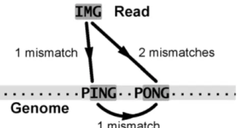
than 0, indeed, some counterintuitive situations might arise, where a read which does not occur in the genome maps uniquely (within the specified edit distance) to a repetitive location having a low mappability. This fact is illustrated with the toy example of Figure 10, where one substitution is used as the maximum allowed edit distance both for computing the mappability and for mapping. With such a choice of parameters the read will map to only one location; yet this position is not unique in the genome, since it has a frequency of 2 (or, equivalently, a mappability score of 1=2). A similar phenomenon happens each time the placement of sequencing errors present in the read forbids the mapping to all copies of a repeated region but one.

In conclusion, knowing that a read maps uniquely to a location is in general not enough to establish, when mismatches are considered, that such a location is unique. In this case, a better indicator for the ‘‘uniqueness of the read’’ is likely to be the theoretical mappability of the region, which has to have been computed separately. The existence of this problem is often overlooked.

Strictly speaking, this not-so-straightforward connection also complicates the (re)definition of expression measures able to take correctly into account the reduced number of unique reads in repetitive loci; however, neither this observation diminishes the

need for such measures, nor it makes less natural and appealing the definition of the RPKUM measure previously presented earlier.

Mappability of paired-end reads

In this last section, we examine how the mappability information can be used together with paired-end/mate-pair sequencing to improve the design of an HTS experiment. In particular, we show that when the mappability is known it is possible to tune the insert size in order to maximize the number of sequencing pairs which one will be able to rescue by resorting to the uniqueness of either end.

When using paired-end reads (or mate-pairs), the mapping information of one end can be used to discard spurious mapping positions of the other end if one takes into account the expected distance between ends imposed by the library size used for sequencing. In consequence, when sequencing with a paired-end type strategy, the paired-end mappability of a position p will be function of both its own single-end mappability and the mappabilities of the positions located at p+(l{k), being l the library size (see Figure 11).

To facilitate the analysis, we have assumed that the standard deviation of the fragment size in each library is zero (that is, all the fragments in the library are having exactly the same size, and hence all the pairs the same distance).

Given the assumptions just presented, it is straightforward to conclude that exactly three cases are possible, as follows (in Figure 11 we illustrate them for the case of paired-end pileup mappability):

1. the single-end mappability of the target position is bigger than, or equal to, the mappabilities of the two possible pairs: the paired-end mappability is not affected by the mappability of the pairs

2. the single-end mappability of the target position is smaller than the mappabilities of one of the pairs: as the new mappability of the target, one can take the average of the single-end mappability of the target and the single-end mappability of that pair

3. the single-end mappability of the target positon is smaller than the mappabilities of the two possible pairs: as the new

Figure 9. Influence of paralogous genes on the mappability scores: the example of the HLA-A gene. The HLA-A gene is part of the Major Histocompatibility Complex (MHC) involving a large gene family with numerous paralogs. This screenshot of the UCSC genome browser (with the six mappability tracks in green) illustrates the low uniqueness of the HLA-A gene (especially, its exon 4) which could render its targeting by RNASeq difficult (if only uniquely mapping reads are considered).

Figure 10. Read mapping and mappability are different concepts: there is no straightforward relation between the number of times a read matches the genome and the mappability of the regions it maps to. Within an edit distance of 1 mismatch, the sequence IMG maps uniquely to location ING in the schematic genome ‘‘...PING-PONG...’’. However, the matched position is not unique in the genome, since considering 1 mismatch it has a frequency of 2 due to location ONG.

(14)

Figure 11. Schematic representation of the computation of the paired-end mappability. In this example the average of the single-end mappabilities at the target position (base C) is bigger than the average of the single-end mappabilities at one of the pairs (base A). Hence the resulting paired-end mappability will be the average of the mean mappabilities at C and A.

Figure 12. Behavior of pileup single-end and paired-end mappabilities at different loci of human chromosome 1 (HSA1). Parameters used to generate this example were: k-mer length 100, 2 mismatches and a library size of 800 bases. Top left: Heatmap of the number of locations in HSA1 as a function of their single-end and paired-end mappabilities. Bottom left: Histogram of the number of locations in HSA1 that show different single-end and paired-end mappabilities, plotted versus their position along the chromosome. Top right: Heatmap of the number of locations in HSA1 as a function of their single-end mappability and their position along the chromosome. Bottom right: Heatmap of the number of locations in HSA1 as a function of their paired-end mappability and their position along the chromosome.

(15)

mappability of the target, one can take the average of the single-end mappabilities of the two possible pairs.

The latter two cases might allow –depending on the single-end mappability of the various loci– to rescue reads which are not by themselves uniquely mappable.

It should be noted that in our calculations we did not take into account paired-end configurations which, while not being unique at any of the pairs, could be still rescued due to the fact that only one of the possible matches for the pair is having the expected insert size. On the contrary, we might be overestimating the mappability of the flanks of regions having long series of tandem repeats: in such a case, a big standard deviation in the sizes of the fragments belonging to a library would complicate the process of identifying a single compatible pair by the expected size of the insert region between the ends, as the problematic reads will have alternative mapping positions very close to each other.

In Figure 12 we present the results of a comparison of single-end and paired-end mappabilities for human chromosome 1 (HSA1) when using a library size of 800 bp. On the heatmap plots one can spot that even when using 100-bp reads the increase in unique mappability can be considerable if the pair information is integrated. Another interesting feature is the distribution of the positions of HSA1 having different single- and paired-end mappabilities: we can clearly identify the centromere position as the one where both mappabilities are the same (and close to zero). Additionally, in order to evaluate the importance of using paired-end information when processing the results of read mapping, we have estimated the single- and paired-end mapp-ability of 100-bp reads for a set of library sizes (300, 400, 500, 600, 700, 800, 900, 1000, 1500, 2000, 4000, 6000, 8000 and 10000 bp) along the whole human genome. To this end, we have estimated which proportion of positions having a non-1 single-end mapp-ability can be rescued completely owing to the fact that both possible pairs in a paired-end experiment are unique. Figure 13 clearly shows that when increasing the library size also the

proportion of reads rescued with this method increases; for large library sizes and some chromosomes (e.g. 3, 4 or 6), such proportion can be higher than 50%.

Remarkably, at small library sizes (v1000 bp) the fraction of rescued reads increases very fast with the distance between the ends. At this scale, the improvement in uniqueness is expected to happen in short regions of the genome (like transposons) which can be seen as unique if they are smaller than the library size, and such that the sequence context around them is itself unique. On the contrary, while for bigger library sizes the percentage of rescued reads keeps growing, the slope of the improvement is much smaller. This result would seem to indicate that in the latter case the repetitive regions we are trying to rescue are much bigger (for instance, this could be the predominant situation for chromosome Y, where the advantage given by such a rescuing strategy turns out to be minimal).

Discussion

In this work, we explore the mappability concept with unprecedented detail, presenting a fast algorithm to compute a well-behaved approximation of the mappability at the level of an entire mammalian genome, even when mismatches are allowed or when small read lengths are used. Our program is freely available, and can be easily used to construct mappability profiles of any given genome. Our visualization tracks of human and mouse mappability profiles are already accessible through the official UCSC genome browser, and more could be uploaded as custom tracks for different model organisms. Auxiliary tracks can be easily derived from the existing ones to account, for instance, for CG-content sequencing bias.

The analysis of the uniqueness of a genome (i.e. the proportion of k-mers having a mappability score of 1) for four model organisms (human, mouse, fly and nematode) computed with up to 2 substitutions revealed a more complex architecture than anticipated. Regions of the genome that are not uniquely

Figure 13. Proportion of completely rescuable positions for all human chromosomes. In this figure we only consider positions having a single-end mappability greater than 1, and for different library sizes (300, 400, 500, 600, 700, 800, 900, 1000, 1500, 2000, 4000, 6000, 8000 and 10000 bp) we plot the fraction of locations which could be rescued by taking advantage of the fact that they have a paired-end mappability equal to one. doi:10.1371/journal.pone.0030377.g013

(16)

mappable correlate not only with the global proportion of repetitive sequences but also, more importantly, with the nature (and hence, the number of copies) of these repeats.

Computing the mappability of a genome is very useful in ChIPSeq experiments, in order to provide a suitable normalization when peaks are scored. In a given RNASeq experiment, calculating a priori the mappability sheds light on regions which will not be easily accessible if multiple mappings are discarded; it could also help to design a better experiment, in particular whenever the main goal is either to exploit most of the biological signal, or to access a specific feature of a genome.

Indeed, we also showed that mappability profiles vary significantly depending on the type of functional element studied and the parameters used (read length and/or number of mismatches). In particular, the analysis of the mappability profiles of gene families (like the olfactory receptors) and pseudo-genes shows that even long HTS reads are not enough to make some features easily accessible: just using a longer read length may not be enough by itself to completely eliminate the ambiguity which arises from the repetitive nature of some interesting features of the genome.

The connection with the design and the analysis of HTS experiments at the level of the single locus is therefore

straightforward. We further emphasized it by examining how mappability impacts the study of single-nucleotide polimorphisms, and how it relates to paired-end sequencing schemes.

Finally, one could note that the systematic fast computation of mappability may be used in various situations of common interest in biology other than those related to the analysis of HTS data – typical examples being the identification of interesting repeated motifs, or the refinement of primer design. Overall, we believe the present work still far from being exhaustive: more and more practical applications of the study of sequence mappability will certainly follow in the future.

Acknowledgments

We would like to thank Rachel Harte from the University of California Santa Cruz for her substantial help in the integration of our mappability tracks into the UCSC Genome Browser.

Author Contributions

Conceived and designed the experiments: TD RG PR. Performed the experiments: TD JE SMS DGK ER PR. Analyzed the data: TD JE DGK ER PR. Contributed reagents/materials/analysis tools: SMS PR. Wrote the paper: TD JE DGK ER RG PR.

References

1. Li H, Homer N (2010) A survey of sequence alignment algorithms for next-generation sequencing. Brief Bioinformatics 11: 473–83.

2. Ribeca P (2008) The GEM (GEnome Multitool) library. URL http:// gemlibrary.sourceforge.net. Accessed 2011 Dec 23.

3. Huda A, Marin˜o-Ramı´rez L, Landsman D, Jordan IK (2009) Repetitive DNA elements, nucleosome binding and human gene expression. Gene 436: 12–22. 4. Feschotte C (2008) Transposable elements and the evolution of regulatory

networks. Nat Rev Genet 9: 397–405.

5. Whiteford N, Haslam N, Weber G, Pru¨gel-Bennett A, Essex JW, et al. (2005) An analysis of the feasibility of short read sequencing. Nucleic Acids Res 33: e171. 6. Rozowsky J, Euskirchen G, Auerbach RK, Zhang ZD, Gibson T, et al. (2009) PeakSeq enables systematic scoring of ChIP-seq experiments relative to controls. Nat Biotechnol 27: 66–75.

7. Rhead B, Karolchik D, Kuhn RM, Hinrichs AS, Zweig AS, et al. (2010) The UCSC Genome Browser database: update 2010. Nucleic Acids Res 38: D613–9. 8. Harrow J, Denoeud F, Frankish A, Reymond A, Chen CK, et al. (2006) GENCODE: producing a reference annotation for ENCODE. Genome Biol 7(Suppl 1): S4.1–9.

9. Burrows M, Wheeler DJ (1994) A block-sorting lossless data compression algorithm. Digital Systems Research Center Research Reports 1: 18. 10. Xavier L. The Objective Caml programming language. URL http://www.

ocaml.org. Accessed 2011 Dec 23.

11. Ohno S (1993) Patterns in genome evolution. Curr Opin Genet Dev 3: 911–4. 12. Cordaux R, Batzer MA (2009) The impact of retrotransposons on human

genome evolution. Nat Rev Genet 10: 691–703.

13. Kazazian HH (2004) Mobile elements: drivers of genome evolution. Science 303: 1626–32.

14. Bailey JA, Eichler EE (2006) Primate segmental duplications: crucibles of evolution, diversity and disease. Nat Rev Genet 7: 552–64.

15. Freeman JL, Perry GH, Feuk L, Redon R, Mccarroll SA, et al. (2006) Copy number variation: new insights in genome diversity. Genome Res 16: 949–61. 16. Ohno S (1987) Repetition as the essence of life on this earth: music and genes.

Haematol Blood Transfus 31: 511–8.

17. Kaminker JS, Bergman CM, Kronmiller B, Carlson J, Svirskas R, et al. (2002) The transposable elements of the Drosophila melanogaster euchromatin: a genomics perspective. Genome Biol 3.

18. Li H, Handsaker B, Wysoker A, Fennell T, Ruan J, et al. (2009) The Sequence Alignment/Map format and SAMtools. Bioinformatics 25: 2078–2079. 19. Wang ET, Sandberg R, Luo S, Khrebtukova I, Zhang L, et al. (2008)

Alternative isoform regulation in human tissue transcriptomes. Nature 456: 470–476.

20. Trapnell C, Williams BA, Pertea G, Mortazavi A, Kwan G, et al. (2010) Transcript assembly and quantification by RNA-Seq reveals unannotated transcripts and isoform switching during cell differentiation. Nature Biotech-nology 28: 511–5.

21. Montgomery SB, Sammeth M, Gutierrez-Arcelus M, Lach RP, Ingle C, et al. (2010) Transcriptome genetics using second generation sequencing in a Caucasian population. Nature 464: 773–7.

22. Du J, Bjornson RD, Zhang ZD, Kong Y, Snyder M, et al. (2009) Integrating sequencing technologies in personal genomics: optimal low cost reconstruction of structural variants. PLoS Comput Biol 5: e1000432.

23. Amaral PP, Dinger ME, Mercer TR, Mattick JS (2008) The eukaryotic genome as an RNA machine. Science 319: 1787–9.

24. Ponting CP, Oliver PL, Reik W (2009) Evolution and functions of long noncoding RNAs. Cell 136: 629–41.

25. Ørom UA, Derrien T, Beringer M, Gumireddy K, Gardini A, et al. (2010) Long noncoding RNAs with enhancer-like function in human cells. Cell 143: 46–58. 26. Marioni JC, Mason CE, Mane SM, Stephens M, Gilad Y (2008) RNA-seq: an assessment of technical reproducibility and comparison with gene expression arrays. Genome Research 18: 1509–17.

27. Morin R, Bainbridge M, Fejes A, Hirst M, Krzywinski M, et al. (2008) Profiling the HeLa S3 transcriptome using randomly primed cDNA and massively parallel short-read sequencing. Biotech 45: 81–94.

28. Li H, Ruan J, Durbin R (2008) Mapping short DNA sequencing reads and calling variants using mapping quality scores. Genome Res 18: 1851–8. 29. Faulkner GJ, Forrest ARR, Chalk AM, Schroder K, Hayashizaki Y, et al. (2008)

A rescue strategy for multimapping short sequence tags refines surveys of transcriptional activity by CAGE. Genomics 91: 281–8.

30. Mortazavi A, Williams BA, Mccue K, Schaeffer L, Wold B (2008) Mapping and quantifying mammalian transcriptomes by RNA-Seq. Nat Meth 5: 621–628. 31. Li B, Ruotti V, Stewart RM, Thomson JA, Dewey CN (2010) RNA-Seq gene

expression estimation with read mapping uncertainty. Bioinformatics 26: 493–500.

32. Wang J, Huda A, Lunyak VV, Jordan IK (2010) A Gibbs sampling strategy applied to the mapping of ambiguous short-sequence tags. Bioinformatics 26: 2501–8.

33. Pas¸aniuc B, Zaitlen N, Halperin E (2011) Accurate estimation of expression levels of homologous genes in RNA-seq experiments. Journal of Computational Biology 18: 459–68.

34. Bailey JA, Gu Z, Clark RA, Reinert K, Samonte RV, et al. (2002) Recent segmental duplications in the human genome. Science 297: 1003–7. 35. Vilella AJ, Severin J, Ureta-Vidal A, Heng L, Durbin R, et al. (2009)

EnsemblCompara GeneTrees: Complete, duplication-aware phylogenetic trees in vertebrates. Genome Res 19: 327–35.

36. Lee S, Seo CH, Lim B, Yang JO, Oh J, et al. (2011) Accurate quantification of transcriptome from RNA-Seq data by effective length normalization. Nucleic Acids Research 39: e9.

37. Smit A, Hubley R, Green P (1996) RepeatMasker Open-3.0. URL http://www. repeatmasker.org. Accessed 2011 Dec 23.Dec 23.