HAL Id: hal-00263507
https://hal.archives-ouvertes.fr/hal-00263507
Submitted on 31 Mar 2009
HAL is a multi-disciplinary open access
archive for the deposit and dissemination of sci-entific research documents, whether they are pub-lished or not. The documents may come from
L’archive ouverte pluridisciplinaire HAL, est destinée au dépôt et à la diffusion de documents scientifiques de niveau recherche, publiés ou non, émanant des établissements d’enseignement et de
Estimation of parameters in incomplete data models
defined by dynamical systems.
Adeline Samson, Sophie Donnet
To cite this version:
Adeline Samson, Sophie Donnet. Estimation of parameters in incomplete data models defined by dynamical systems.. Journal of Statistical Planning and Inference, Elsevier, 2007, 137 (9), pp.2815-2831. �10.1016/j.jspi.2006.10.013�. �hal-00263507�
Estimation of parameters in incomplete data
models defined by dynamical systems
Sophie Donnet
1, Adeline Samson
21 Paris-Sud University, Laboratoire de Math´ematiques, Orsay, France 2 INSERM U738, Paris, France; University Paris 7, Paris, France
Abstract
Parametric incomplete data models defined by ordinary differential equa-tions (ODEs) are widely used in biostatistics to describe biological processes accurately. Their parameters are estimated on approximate models, whose regression functions are evaluated by a numerical integration method. Ac-curate and efficient estimations of these parameters are critical issues. This paper proposes parameter estimation methods involving either a stochas-tic approximation EM algorithm (SAEM) in the maximum likelihood es-timation, or a Gibbs sampler in the Bayesian approach. Both algorithms involve the simulation of non-observed data with conditional distributions using Hastings-Metropolis (H-M) algorithms. A modified H-M algorithm, including an original Local Linearization scheme to solve the ODEs, is pro-posed to reduce the computational time significantly. The convergence on the approximate model of all these algorithms is proved. The errors induced by the numerical solving method on the conditional distribution, the likelihood and the posterior distribution are bounded. The Bayesian and maximum likelihood estimation methods are illustrated on a simulated pharmacoki-netic nonlinear mixed-effects model defined by an ODE. Simulation results illustrate the ability of these algorithms to provide accurate estimates.
KEYWORDS: Bayesian estimation, Incomplete data model, Local lin-earization scheme, MCMC algorithm, Nonlinear mixed-effects model, ODE integration, SAEM algorithm
1
Introduction
When a biological or physiological process is measured, the regression func-tion of the statistical model corresponding to the observed data is often de-rived from a differential equation describing the underlying dynamic process. Difficulties arise when the differential equation has no analytical solution and/or when the parameters of the regression function are random and thus non-observed. Such example can be found in pharmacokinetics, which aims to study drug evolutions in human organism, this evolution being described by differential systems of compartment interactions. Mixed models, for which regression parameters are considered as random variable and non-observed data, are widely used for the analysis of pharmacokinetic datasets, which have classically repeated measurements in several patients.
This paper aims at providing a general answer to the estimation problem in such statistical incomplete data models.
Let y be the noised observations of a biological process measured at in-stants (t1,· · · , tJ). The biological process is described by the solution g
of an ordinary differential equation (ODE), depending on a stochastic non-observed parameter φ:
yj = g(tj, φ) + εj for j = 1· · · J.
We consider that the observable vector Y is part of a so-called complete vector (Y, φ). We assume that both Y and (Y, φ) have density functions, pY(y; θ) and pY,φ(y, φ; θ) respectively, depending on a parameter θ belonging
to some subset Θ of the Euclidean spaceRq. The estimation of the parameter
θ has been widely studied when the regression function g has an explicit form. Two approaches can be followed to tackle this challenge, respectively the maximum likelihood and the Bayesian estimations.
Generally, the maximization of the likelihood of the observations can-not be done in a closed form. Dempster et al. (1977) propose the itera-tive Expectation-Maximization (EM) algorithm for incomplete data prob-lems. At the kth iteration, the E-step of EM algorithm computes Q(θ|θ
k) =
For cases where the E-step has no closed form, stochastic versions of EM are introduced. Celeux and Diebolt (1985) introduce the Stochastic EM algo-rithm (SEM). Wei and Tanner (1990) suggest the Monte-Carlo EM (MCEM) estimating Q(θ|θk) by the averaging of m Monte-Carlo replications. Recently,
Wu (2004) emphasizes that MCEM is computationally intensive. As an al-ternative, Delyon et al. (1999) propose the Stochastic Approximation EM algorithm (SAEM) replacing the E-step by a stochastic approximation of Q(θ|θk). These methods require the simulation of the non-observed data φ.
For cases where this simulation can not be performed in a closed form, Kuhn and Lavielle (2004) suggest to resort to iterative methods such as Monte Carlo Markov Chain algorithms (MCMC).
The Bayesian approach estimates the posterior distribution pθ|Y(·|y) of θ,
a prior pθ(·) being given. Because of the conditional independence structure
of pθ|Y =
!
pθ|Y,φ pφ|Y dφ and pφ|Y =
!
pφ|Y,θ pθ|Y dθ, Gelfand and Smith
(1990) propose a Gibbs sampling to evaluate these two integrals simultane-ously. At iteration k, φk, a realization of φ, is simulated with pφ|Y(·, θk−1)
followed by θk, a realization of θ with pθ|Y,φ(·, φk). Consequently, as in
maxi-mum likelihood estimation, difficulties arise when the simulation of the con-ditional distribution can not be performed in a closed form. For these cases, a Hastings-Metropolis (H-M) algorithm can be included in the Gibbs sampler. The use of the H-M algorithm in estimation algorithms requires the evalu-ation of the regression function g at each iterevalu-ation. When g is a non-analytical solution of a dynamical system, it is evaluated using a numerical integration method. Thus a trade-off between accuracy, stability and computational cost is required. In this paper, we detail the Local Linearization scheme (see e.g. Biscay et al., 1996; Ramos and Garc´ıa-L´opez, 1997; Jimenez, 2002) not only because of its stability performances but also because this scheme can be extended to a so-called modified Local Linearization scheme, adapted to its inclusion in the H-M algorithm. The estimation algorithms are then ap-plied to an approximate model whose regression function is an approximate solution of the ODE.
The objective of this research is to quantify the error induced by the numerical approximation of the regression function g. The paper is orga-nized as follows. Section 2 defines the original statistical model; the Local Linearization scheme and its modified version are detailed; the approximate statistical model resulting from the numerical approximation is introduced. Section 3 focuses on the H-M algorithm to simulate the non-observed data φ with the conditional distribution. The error induced by the numerical
approximation of g on the conditional distribution is quantified. Section 4 is dedicated to the parameter estimation algorithms. Concerning maximum likelihood and Bayesian estimations, the standard algorithms are adapted to solve the approximate model. The error induced by the use of the numerical solving method is bounded respectively on the likelihood and the posterior distribution. This error is distinct from the error on the estimates induced by the estimation algorithm which is evaluated by their standard errors. Fi-nally, the SAEM algorithm and the Bayesian Gibbs sampler are applied on a nonlinear mixed-effects model deriving from pharmacokinetics in Section 5.
2
Models and notations
2.1
An incomplete data model defined by ODEs
Let y = (yj)j=1..J denote the observations measured at times (t1,· · · , tJ). We
consider the incomplete data model, called model M, defined as follows: yj = g(tj, φ) + εj 1≤ j ≤ J
εj ∼ N (0, σ2) (M)
φ ∼ π(·; β)
where g(.) is a nonlinear function of φ, εj represents the error of the
measure-ment j, σ2 is the residual variance, φ is a non-observed random parameter
distributed with the density π(·, β), depending only on the parameter β. The parameter θ = (β, σ2) belongs to some open subset Θ⊂ Rq.
Let g be written g = H◦ f, where H : Rd−→ R is a known function and,
f : R × Rk−→ Rd is defined as the solution of the following ODE:
∂f (t, φ)
∂t = F (f (t, φ), t, φ) (1)
f (t0, φ) = f0(φ)
with a known function F : Rd× R × Rk −→ Rd and the initial condition
f0(φ)∈ Rd, t∈ [t0, T ].
We make the following additional assumptions:
• Assumption H1: π has a compact support K1 ⊂ Rk, and there exist
two constants a and, b such that
• Assumption H2: F : Rd×R×Rk−→ RdisC2 on its definition domain,
and φ−→ f0(φ)∈ Rk isC1 on K1.
• Assumption H3: H is an LH-lipschitzian function.
2.2
Approximation of the regression function
A great variety of numerical schemes have been proposed to solve ODEs (see e.g. Hairer et al., 1987). The accuracy of such numerical methods is qualified by the order and the step size of these schemes. The numerical scheme is applied on sub-intervals [tn, tn+1[, n = 0, . . . , N − 1, of the time interval
[t0, T ], with tN = T . The maximal length or step size of the sub-intervals is
denoted h. The order of a numerical scheme is defined as follows:
Definition 1 Let fh be the resulting approximate function obtained by a
nu-merical integration scheme of step size h. This scheme is of order p if there exists a constant C such that
sup
t∈[t0,T ]
|f(t, φ) − fh(t, φ)| ≤ Chp.
Of all the numerical schemes, the Local Linearization (LL) scheme pro-vides a good trade-off between computational cost and numerical stability, as exposed in Biscay et al. (1996). It derives from the local linearization of the right term of the ODE (1) with respect to time t, and the exact integration of the deduced linear differential equation. Its implementation requires matrix exponential computations using new algorithms such as Pade or Schur meth-ods, which have proved their efficiency and stability. The LL scheme has the additional advantage of preserving stability properties on stiff systems (see e.g. Ramos and Garc´ıa-L´opez, 1997; Jimenez et al., 2002). In cases where the ODE depends on parameter φ, we extend this scheme using a Taylor expansion with respect to time t and parameter φ. More precisely, let the solution at φ0 be computed using the LL scheme. Let φ be in a neighborhood
of φ0. On each sub-interval [tn, tn+1[, n = 0, . . . , N − 1, the solution fh,φ0 of
the following linear equation ∂f (t, φ) ∂t = F (f (tn, φ0), tn, φ0) + dF df (f (tn, φ0), tn, φ0) (f (t, φ)− f(tn, φ0)) +dF dt (f (tn, φ0), tn, φ0) (t− tn) + dF dφ (f (tn, φ0), tn, φ0) (φ− φ0).
is evaluated. Details of this scheme (called LL2 scheme) are given in appendix B. This LL2 scheme does not involve any additional computation of matrix exponentials: the required matrix exponential has already been computed with the LL scheme at φ0. This reduces the computational time, which is a
key issue in iterative processes. For instance, during H-M algorithm imple-mentation, the ODE has to be integrated at φ contained in a neighborhood of φ0, for which the ODE has already been solved by LL. This leads us to
propose a modified version of the H-M algorithm, taking advantage of these schemes (see Section 3).
Convergence properties of the two previous numerical schemes are given in the following lemma. Let us consider the following assumption:
• Assumption H1#: φ remains in the compact set K
1 ∈ Rk.
Lemma 1 Let φ0 and φ be in K1. Let f (., φ) be the exact solution of the
ODE (1), fh(., φ) the one obtained by the LL scheme with step size h, and
fh,φ0(., φ) the LL2 solution. Assume that H1# and H2 hold. Then:
1. there exists a constant C independent of φ, such that, for any t∈ [t0, T ]
and for any φ,
|f(t, φ) − fh(t, φ)| ≤ Ch2,
2. there exist constants C1 and C2 such that, for any t ∈ [t0, T ] and for
any φ,
|f(t, φ) − fh,φ0(t, φ)| ≤ max(C1h
2, C
2)φ − φ0)2Rk).
Part 1 is proved in Ramos and Garc´ıa-L´opez (1997), part 2 is proved in appendix B.
2.3
An approximate incomplete data model
In practice, estimation algorithms require the numerical approximation of the regression function and are thus applied to an approximate version of the modelM. Let fh be the approximate solution of the ODE (1), obtained by a
numerical integration method of step size h and order p. Let the approximate statistical model Mh be defined by:
yj = gh(tj, φ) + εj 1≤ j ≤ J
εj ∼ N (0, σ2) (Mh)
where gh = H ◦ fh. Subsequently, the different distributions of the model
Mh are subscripted with h.
3
Simulation of non-observed data with the
conditional distribution
In this paper, the Hastings-Metropolis (H-M) algorithm is combined succes-sively with the SAEM algorithm in the maximum likelihood estimation, and the Gibbs sampler in the Bayesian estimation. The H-M algorithm updates φ in the target distribution p(φ|y; θ). The computation of its acceptance probabilities requires an explicit expression of the regression function. As a consequence, this H-M algorithm can only be applied to the approximate statistical model Mh.
The standard H-M algorithm and a modified version of the random-walk H-M algorithm including the LL2 scheme leading to computational time sav-ings in practice, are presented in Section 3.1. Section 3.2 presents the con-vergence of the algorithms.
3.1
The Hastings-Metropolis algorithm
The iterative H-M algorithm implemented on model Mh generates a Markov
chain with the target distribution ph(φ|y; θ) as invariant distribution and
using a proposal density q. At step r + 1, given φ(r):
• Generate a candidate φc from the proposal density q(.|φ(r)).
• Generate U ∼ U([0, 1]). Then, φ(r+1) = " φc if U < ρ(φ(r), φc), φ(r) if U > ρ(φ(r), φc), where ρ(φ(r), φc) = min " 1, ph,φ|Y(φ c) ph,φ|Y(φ(r)) q(φ(r)|φc) q(φc|φ(r)) # is the acceptance probability.
The choice of the proposal density q is essentially arbitrary, although in practice a careful choice will help the algorithm to move quickly inside the pa-rameter space. Two proposal densities are combined. First the prior density q(.|φ(r)) = π(.; β) allows to move inside the parameters space efficiently.
Sec-ond, a symmetric distribution q(φc|φ(r)) = q(φ(r)|φc) is used resulting in the
so-called random-walk H-M algorithm (see e.g. Bennet et al., 1996). In this case, φc = φ(r)+ δ with δ simulated from a centered symmetric distribution
such that φc remains in K 1.
Remark 1 In practice, the random-walk H-M algorithm can be modified to reduce the computational time using the LL2 scheme. Indeed, on the model Mh defined by the LL scheme, the random-walk H-M algorithm requires
solv-ing the ODE (1) at φc in a bounded neighborhood of φ(r), for which the LL
approximate solution has been computed.
Let the centered symmetric proposal density verify the following property, called property (2): there exists η > 0 such that, almost surely,
)φ(r)− φc)
Rk < η. (2)
The modified H-M algorithm including the LL2 scheme is outlined as followed. At step r + 1, given φ(r),
• Generate a candidate φc = φ(r)+ δ
• Accept φc with probability ρ(2)(φ(r), φc) where
ρ(2)(φ(r), φc) = min $ 1, p (2) h,φ|Y(φc) ph,φ|Y(φ(r)) q(φ(r)|φc) q(φc|φ(r)) % = min $ 1, p (2) h,Y|φ(φc)π(φc) ph,Y|φ(φ(r))π(φ(r)) %
and p(2)h,Y|φ(.) is evaluated using the LL2 scheme.
If the move is accepted fh(t, φ(r+1)) and the ph,Y|φ(φ(r+1)) density are
re-evaluated using the LL scheme. If it is not accepted no additional matrix exponential is computed, significantly reducing the computational time.
3.2
Convergence
The convergence of the standard H-M algorithm and the error induced by the numerical integration scheme are studied in Theorem 1.
Theorem 1 Let f be the exact solution of ODE (1). Let pφ|Y be the
condi-tional distribution for the modelM. Assume that H1, H2 and H3 hold. Let fh be the approximate solution obtained by a numerical integration method
of step size h and order p. Let ph,φ|Y be the conditional distribution of the
model Mh.
1. Then on the model Mh, the H-M algorithm converges towards its
sta-tionary distribution ph,φ|Y.
2. Furthermore, there exists a constant Cy such that for any small h,
D(pφ|Y, ph,φ|Y)≤ Cyhp.
where D(·, ·) denotes the total variation distance.
The rates of convergence of the standard H-M algorithms have been widely studied (see e.g. Tierney, 1994), hence are not discussed here.
Remark 2 The modified H-M algorithm based on the LL2 scheme results in a non standard form of the acceptance probability due to the two approxima-tions of the target distribution. Thus, the proof of its convergence is complex and beyond the scope of this paper. In cases where the modified H-M algo-rithm converges to a stationary distribution p(2)h , provided the property (2) is checked and the chain (φ(r)) remains in K
1, there exists a constant Cy(2) such
that D(pφ|Y, p(2)h )≤ Cy(2)η + Cyh2.
The proofs of theorem 1 and the previous inequality are given in appendix A. Numerical illustrations are given in Section 5.
4
Estimation of parameters
In the following section, we extend to incomplete data models defined by ODEs, the SAEM algorithm coupled with the H-M algorithm for the maxi-mum likelihood estimation, and the Gibbs sampling algorithm for the Bayesian approach, to estimate the parameters θ = (β, σ2).
4.1
Maximum likelihood approach
The EM algorithm proposed by Dempster et al. (1977) maximizes the Q(θ|θ#) =
E(log pY,φ(·; θ)|y; θ#) function in two steps. At the kth iteration, the E-step
is the evaluation of Qk(θ) = Q(θ| θk) while the M-step updates θk by
maxi-mizing Qk(θ). For cases where the E-step has no closed form, Delyon et al.
(1999) introduce a stochastic version SAEM of the EM algorithm. The Qk(θ)
integral is evaluated by a stochastic approximation procedure. The E-step is divided into a simulation step (S-step) of the non-observed data φk with
the conditional distribution pφ|Y(.; θk) and a stochastic approximation step
(SA-step):
Qk+1(θ) = Qk(θ) + γk(log(pY,φ(.; θk))− Qk(θ)) ,
where (γk) is a sequence of positive numbers decreasing to 0. They prove
the convergence of this algorithm under general conditions in the case where pY,φ belongs to a regular curved exponential family. When the non-observed
data cannot be directly simulated, Kuhn and Lavielle (2004) suggest using a MCMC scheme by building a Markov chain with pφ|Y(·; θk) as unique
sta-tionary distribution at the kth iteration.
When the regression function is defined by ODE, SAEM is implemented on the model Mh. Let π(·, β) be such that ph,Y,φ belongs to the exponential
family:
ph,Y,φ(·; θ) = exp {−Ψ(θ) + *Sh(y, φ), Φ(θ)+} ,
where ψ and Φ are two functions of θ,*·, ·+ is the scalar product and Sh(y, φ)
is known as the minimal sufficient statistics of the complete model, taking its value in a subsetS of Rm. Let π(·; β) be of class Cm. At the kth iteration,
the SAEM algorithm is:
• S-Step: the non-observed data φk is simulated by the H-M algorithm
developed in section 3 with ph,φ|Y(·; θk) as unique stationary
distribu-tion,
• SA-Step: sk+1 is updated by the stochastic approximation:
sk+1 = sk+ γk(Sh(y, φk)− sk),
• M-Step: θk is updated by
θk+1 = arg max θ
Kuhn and Lavielle (2004) propose estimates of the Fisher information matrix, using the Louis’s missing information principle (Louis, 1982), either by importance sampling or by stochastic approximation. We adapt their estimates when the regression function is not known analytically and, as a consequence, the extended SAEM supplies the standard errors of the esti-mates.
The convergence of SAEM is proved on Mh and the distance between
the likelihoods of the two models is quantified in the following theorem. Theorem 2 Let us consider a numerical scheme of step size h and order p. Let H1, H2 and H3 hold. Let (γk) be a sequence of positive numbers
decreasing to 0 such that for any k in N, γk ∈ [0, 1], &∞k=1γk = ∞ and
&∞
k=1γk2 <∞.
1. Assuming the sequence (sk)k≥0 takes its values in a compact set of S,
the sequence (θk)k≥0obtained by the SAEM algorithm onMh, converges
almost surely towards a (local) maximum of the likelihood ph,Y(y).
2. For any σ2
0 > 0, there exists a constant θ-independent C such that
sup
θ=(β,σ2)|σ2>σ2 0
|pY(y; θ)− ph,Y(y; θ)| ≤ Chp.
Hence, as a principal consequence of this theorem, and assuming regularity hypotheses on the Hessians of the likelihoods of both models M and Mh,
the bias of the estimates induced by both the numerical approximation and the estimation algorithm, is controlled.
Proof 1 1. Assumptions of convergence of the SAEM algorithm are checked by the model Mh. See Kuhn and Lavielle (2004) for more details.
2. In the proof of theorem 1, we obtain the result (1b) for a fixed θ and small enough h that:
|pY(y; θ)− ph,Y(y; θ)| ≤
Cy
(2πσ2)J/2h p.
Consequently, for any σ2
0 > 0, for any θ ∈ Θ with σ2 ≥ σ20, there exists
a constant C, independent of θ, such that
4.2
Bayesian approach
The Bayesian model is defined as follows:
yj = g(tj, φ) + εj 1≤ j ≤ J
εj ∼ N (0, σ2)
φ ∼ π(·; β) θ ∼ pθ(·; Γ)
where θ = (β, σ2) is distributed from the prior distribution p
θ with fixed
hyperparameters Γ. For example, a Gamma prior distribution can be chose for σ−2. The prior distribution on β depends on the specific distribution π.
The Bayesian approach consists in the evaluation of the posterior distribu-tion pθ|Y. The iterative Gibbs sampling algorithm is outlined as follows (see
Huang et al., 2004, for more details):
• Step 1: initialize the iteration counter of the chain k = 1 and start with initial values σ−2(0), β(0), φ(0).
• Step 2: obtain a new value σ−2(k), β(k), φ(k)from σ−2(k−1), β(k−1), φ(k−1)
through successive generation of values
1. σ−2(k) ∼ p(σ−2|β(k−1), φ(k−1), y) β(k)∼ p(β|σ−2(k), φ(k−1), y)
2. φ(k) ∼ p(φ|σ−2(k), µ(k), Ω(k), y)
• Step 3: change the counter from k to k +1 and return to Step 2 until convergence is reached.
For a Gamma prior distribution on σ−2, the conditional distribution
p(σ−2|β(k−1), φ(k−1), y) is a Gamma distribution. The conditional
distribu-tion p(β|σ−2(k), φ(k−1), y) depends on the specific form of the distribution
π(.; β). To generate a realization of φ, Bennet et al. (1996) describe sev-eral approaches, such as a Rejection Gibbs, a Ratio Gibbs, independent or Random-walk H-M algorithms. Gilks et al. (1996) recommend the use of initial iterations allowing a ”burn-in” phase, followed by a large number of iterations.
For models defined by ODEs, the inclusion of such H-M algorithms re-quires the evaluation of g(φ, tj) at each iteration. Hence, the Gibbs algorithm
In practice, we estimate the posterior distribution of the model Mh
in-stead of the distribution of interest pθ|Y. The following theorem quantifies
the total variation distance between the posterior distribution ph,θ|Y and this
original distribution of interest, pθ|Y.
Theorem 3 Let us consider a numerical scheme of step size h and order p. Let pθ|Y and ph,θ|Y be the posterior distributions respectively of M and Mh.
Assume that H1, H2 and H3 hold.
1. The Gibbs sampling algorithm converges on the model Mh.
2. There exists a y-dependent constant Cy such that
D(ph,θ|Y, pθ|Y)≤ Cyhp.
Hence, as a principal consequence of this theorem, the bias on the posterior mean is controlled: under moments hypotheses on pθ(θ) and ph,θ|Y(θ), there
exists a constant Cy# such that
' 'Eθ|y(θ)− Eh,θ|y(θ) ' ' =''! θpθ|Y(θ)dθ− ! θph,θ|Y(θ)dθ ' ' ≤ C#
yhp where Eθ|y(·) and Eh,θ|y(·) are the expectation under the posterior
dis-tributions pθ|y and ph,θ|y respectively. Similar result can be obtained for the
bias of the posterior mode, assuming regularity hypotheses on the distribu-tions pY|θ and ph,Y|θ of both models M and Mh.
Proof 2 1. Assumptions of convergence of the Gibbs sampling algorithm are checked on the model Mh, see Carlin and Louis (2000) for more
details.
2. By Bayes theorem, we have
pθ|Y =
pY|θpθ
pY
where pY =
!
pY|θpθdθ, and the same equality for the modelMh. From
the result (1b) of the proof of theorem 1, we deduce that there exists a constant C, independent of θ, such that for any θ ∈ Θ with σ2 > σ2
0 > 0,
|pY|θ(y)−ph,Y|θ(y)| ≤ Chp and|pY(y)−ph,Y(y)| ≤ Chp. We now bound
|pθ|Y(θ)− ph,θ|Y(θ)|: |pθ|Y(θ)− ph,θ|Y(θ)| ≤ pθ(θ) |pY(y)| ' ' '
'|pY|θ(y)− ph,Y|θ(y)| +
pY(y)
ph,Y(y)|p
Y(y)− ph,Y(y)|
' ' ' ' ≤ Ch p |pY(y)| pθ(θ) ' ' '
'1 + pph,Yh,Y|θ(y)(y) ' ' ' ' = Ch p |pY(y)| ( pθ(θ) + ph,θ|Y(θ) ) .
Thus
D(pθ|Y, ph,θ|Y)≤ Ch
p
|pY(y)|
.
5
Application to nonlinear mixed-effects model
Nonlinear mixed-effects models are widely used in pharmacokinetics (PK) and pharmacodynamics (PD) to estimate PK/PD parameters. They are interesting because of their capacity to discriminate the intra- from the inter-subject variabilities and to test covariate effect on the PK/PD parameters. They are modeled by:
yij = C(tij, φi) + εij
εij ∼ N (0, σ2)
φi ∼ π(.; β),
where yij is the observation of the drug concentration C for subject i, i =
1, . . . , N , at time tij, j = 1, . . . , ni and φi is the vector of individual
non-observed PK/PD parameters of subject i. A Gaussian distribution π(.; β) = N (µ, Ω) is classically chosen for φ, resulting in β = (µ, Ω). In the Bayesian framework, Gamma prior distribution is chosen for σ−2, Wishart or Gamma
prior distribution is chosen for Ω−1 and a Gaussian prior distribution is used for µ.
We consider a case where the drug concentration C is defined through a differential equation without analytical solution. On a simulated dataset, we illustrate applications of the H-M, the SAEM and the Bayesian Gibbs algorithms.
5.1
Numerical settings
The following one-compartment pharmacokinetic system with a first order absorption and a Michaelis-Menten saturable elimination describes the con-centration C of a drug: dC dt (t, φ) = kaD V e −kat− VmC(t, φ) km+ C(t, φ) , (3)
where D is the known administered dose, V the total volume of distribu-tion, ka the absorption constant, km the Michaelis-Menten constant and
Vm the maximum rate of metabolism. Hence, the parameter vector is φ =
[V, ka, km, Vm]∈ R4.
We consider the pharmacokinetic parameters of hydroxurea, an anti-cancerous drug, studied by Tracewell et al. (1995): V =12.2 L, ka=2.72
h−1, k
m=0.37 mmol/L, Vm=0.082 mmol/h/L. One dataset of 20 patients
is simulated with a dose D = 13.8 mmol and measurements at time t = 0, 0.5, 1, 1.5, 2 hours and then every hour until 12 hours. We choose a Gaus-sian distribution for φ with a diagonal variance-covariance matrix (diagonal components equal to 0.4). The residual variance σ2 is set to 0.01. The
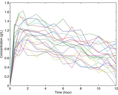
nu-merical method used to simulate this dataset is the ode45 solving Matlab function, that implements a Runge-Kutta scheme of the fourth order, with a very small maximal step size of resolution h equal to 0.001. Data are plotted on figure 1.
[Figure 1 about here.]
5.2
Results
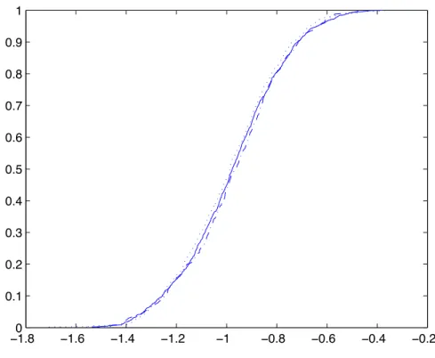
Several numerical integration methods included in the H-M algorithm are compared on the simulation of the conditional distributions. 1000 inde-pendent 200-long Markov chains are generated for each method. The first method is the ode45 function with maximal step size h = 0.001 in order to obtain an exact cumulative distribution function; this is the reference as this numerical method is of the fourth order with a very small step size. Then we compare the two cumulative distribution functions obtained by using at first ode45 with the default step size h = 0.1 and then the LL and LL2 schemes. As seen on Figure 2, plotting the empirical cumulative distribution functions, the three numerical methods provide similar simulated conditional distributions.
[Figure 2 about here.]
The SAEM and Bayesian Gibbs algorithms are applied to the simulated dataset. We implemented the SAEM algorithm in Matlab and the Bayesian Gibbs algorithm is the one implemented in WinBugs and its Differential Interface software (Spiegelhalter et al., 1996). These estimates are com-pared with those obtained by the NONMEM software, proposed by Beal and Sheiner (1982) and used by 80% of the pharmacokineticists in drug compa-nies. NONMEM is an implementation of the First Order Conditional Esti-mate algorithm, which is based on a first order linearization of the regression
function around the conditional estimates of the parameters φ, the standard errors of the estimates being evaluated by linearization.
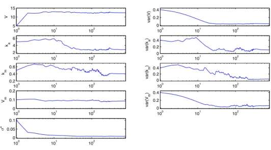
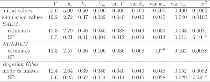
Initial values have been arbitrarily chosen and are presented in Table 1. The evolutions of each SAEM parameter estimate are plotted against iterations on Figure 3. The estimates converge rapidly to a neighborhood of the simulated values.
[Figure 3 about here.]
In the Bayesian framework, a Gamma prior distribution has first been used on Ω−1 leading to unacceptable convergence graphs. A Wishart prior distri-bution has then been used on Ω−1with satisfactory convergence and posterior
density graphs after 100000 iterations.
The parameter estimates and their standard errors obtained by SAEM, NONMEM and the Bayesian Gibbs algorithms are presented in Table 1.
[Table 1 about here.]
In this example, it takes about ten minutes for SAEM to converge us-ing a conventional Intel Pentium IV 3,2 GHz workstation. All the SAEM estimates almost reach the simulated values. The SAEM algorithm achieves the evaluation of the information Fisher matrix, and almost all the standard errors of the estimates are satisfactory. Using the same computer, the NON-MEM software stops after about ten minutes without convergence towards the maximum of the likelihood. The estimate of Vm does not change from
its initial value, the estimate of km is far from its simulation value, var km is
estimated near zero while var Vm and var ka are overestimated. The
NON-MEM software fails to evaluate the standard errors of all estimates. Using the same computer, it takes about one hour for the Winbugs software to compute 100 000 iterations of one Markov chain of the Gibbs algorithm. All the Bayesian estimates almost reach the simulated values and the standard errors of the estimates are satisfactory.
This simulated example illustrates the ability of the proposed algorithms to estimate precisely the parameters of mixed models defined by ODE.
6
Discussion
This paper extends the statistical approaches used to estimate incomplete data model parameters to the frequent cases where such a model M is de-fined by a dynamical system. To that purpose, an approximate model Mh is
introduced, of which regression function is evaluated by a numerical integra-tion method. The standard estimaintegra-tion algorithms are adapted to estimate this approximate model. The convergence of the H-M, the SAEM and the Gibbs Sampling algorithms on the model Mh is proved.
This paper quantifies the error induced by the use of a numerical solving method. The errors on the conditional distribution, the likelihood and the posterior distribution between the modelM and the approximate model Mh
are controlled by hp, where h is the step size and p the order of the numerical
integration method. This error is distinct from the error on the estimates induced by the estimation algorithms, which is classically controlled by the standard errors evaluated through the Fisher information matrix of the esti-mates.
This paper proposes an extended version of the LL scheme, using the de-pendence to the parameter φ of the ODE, which allows to reduce significantly the computational cost of the H-M algorithm in practice. The major advan-tage of the LL schemes is its behavior on stiff dynamical systems, providing an interesting trade-off between computational cost and numerical stability when included in an iterative stochastic algorithm Biscay et al. (1996).
Regarding the maximum likelihood, we study the SAEM algorithm in-stead of the Monte-Carlo EM proposed by Wei and Tanner (1990) or Wu (2004). With an analytical regression function, the MCEM is computational intensive because of the large sample of non-observed data simulated at each iteration, while the Stochastic Approximation method requires the genera-tion of only one realizagenera-tion of non-observed data at each iteragenera-tion. Thus, due to computational time considerations, we only extend the SAEM algorithm to the case of regression function implicitly defined.
The SAEM algorithm is applied to a dataset simulated using a pharma-cokinetic model defined by ODEs. The SAEM estimates are compared with those obtained by the standard estimation software NONMEM, the only available software providing estimates by maximum likelihood in nonlinear mixed models defined by ODEs. SAEM provides satisfying estimates and standard errors of the parameters, while NONMEM does not converge on this simulated example and fails to evaluate the standard errors. The esti-mation algorithm implemented in NONMEM is based on the linearization of the regression function. Despite the fact that Vonesh (1996) highlights problems of consistence and convergence of the estimates produced by such estimation methods, NONMEM is used by 80% of the pharmacokineticists in the pharmaceutical industry. The simulation results presented in this paper
point out the poor ability of this software to estimate the parameters in non-linear mixed model defined through ODEs. Thus we recommend using the SAEM algorithm to analyze such incomplete data problems defined by ODE. The SAEM algorithm is implemented by the MONOLIX group in a free Mat-lab function (http://mahery.math.u-psud.fr/∼lavielle/monolix/index.html). The extension of the monolix function to ODE models will soon be available on the same web-site.
Several methods have been suggested to simulate the non-observed data included in a Bayesian approach. Wakefield et al. (1994) sample the non-observed data using a ratio-of-uniform while Tierney (1994) proposes using a Hastings-Metropolis algorithm. Gilks et al. (1996) summarize these methods in their book. We use the Winbugs software and its Differential Interface software Spiegelhalter et al. (1996), which implements hybrid Gibbs and Hastings-Metropolis algorithms. On the simulated dataset, the posterior distributions are well estimated while the subject number was low.
In this paper, the methodology is illustrated on a mixed model issued from pharmacocinetics. However, there exist many others fields of applica-tions. First, it can be applied in Functional Magnetic Resonance Imaging (fMRI), a neuroimaging technique using the vascular oxygenation contrast as an indirect measure of cerebral activity. Despite the extensive develop-ment of such techniques, the coupling mechanisms between neuronal activity and cerebral physiological changes -such as vascular changes- are still poorly understood. Recently, dynamical models such as the Balloon model have been introduced to explain these interactions (Buxton et al., 1998), leading to define statistical models defined by ODEs. Many others applications can be found in the framework of functional data analysis in the case where the underlying process can be described by a differential system.
Diffusion models described by stochastic differential equations (SDEs) are natural extensions to the corresponding deterministic models (defined by ODEs) to account for time-dependent residual errors and to handle real life variations in model parameters occurring over time. The two estimation methods proposed in this paper can be extended to this case, opening wide perspectives of application.
Acknowledgements
The authors are grateful to their advisor Professor Marc Lavielle for his constructive advice and help. The authors thank Professor France Mentr´e for her helpful comments. The authors would like to thank Rolando Biscay for helpful discussions about Local Linearisation schemes and Jean-Louis Foulley for his constructive help about Bayesian estimation.
A
Convergence of the H-M:
1. Proof of Theorem 1
(a) Following Tierney (1994), the H-M algorithm provides a uniformly ergodic Markov chain with ph,φ|Y as invariant distribution, as soon
as π is one of the proposal density.
(b) By Bayes theorem, we have pφ|Y(φ) = pY|φ(y|φ)π(φ)
pY(y) , and
'
'pφ|Y(φ)− ph,φ|Y(φ)'' = π(φ) pY(y)
*''p
Y|φ(y)− ph,Y|φ(y)
'
' +ph,Y|φ(y)
ph,Y(y) |p
Y(y)− ph,Y(y)|
+ . We have ''pY|φ(y|φ) − ph,Y|φ(y|φ) ' ' = |pY|φ(y)| ' ' '1 −ph,Y|φ(y) pY|φ(y) ' ' ', and pY|φ(y) = 1 (2πσ2)J/2 exp , − 1 2σ2 J -j=1 (yj − g(tj, φ))2 . . Furthermore, by H3, we have: |gh(t, φ)− g(t, φ)| = |H ◦ fh(t, φ)− H ◦ f(t, φ)| ≤ LHsup t,φ |f h(t, φ)− f(t, φ)| ≤ LHChp.
By H1 and the assumptions on the proposal densities, (t, φ) re-mains a.s. uniformly in the compact set [t0, T ]× K1. Thus there
exist M and, Mh such that
M = sup
(t,φ)∈[t0,T ]×K1
|g(t, φ)| , Mh = sup (t,φ)∈[t0,T ]×K1
and, we can prove that Mh ≤ M + Chp. Hence, there exists Ah such that ' '(yj− gh(tj, φ))2 − (yj− g(tj, φ))2 ' ' ≤ AhChp
and, we obtain a φ-independent bound: '
'pY|φ(y)− ph,Y|φ(y)
' ' ≤ 1 (2πσ2)J/2(e 1 2σ2JAhCh p −1) ≤ (2πσ12)J/2 (eBAhhp− 1), with B = JC
2σ2. Consequently, by integrating the previous
inequal-ity,
|pY(y)−ph,Y(y)| ≤
/ '
'pY|φ(y)− ph,Y|φ(y)
'
' π(φ)dφ ≤ 1
(2πσ2)J/2(e
BAhhp−1).
Finally, using the previous inequalities, we have: / ' 'pφ|Y(φ)− ph,φ|Y(φ) ' ' dφ ≤ 2 pY(y)(2πσ2)J/2 (eBAhhp− 1).
Let D(·, ·) denote the total variation distance. If h is small enough, there exists a h-independent constant Cy such that:
D(pφ|Y, ph,φ|Y)≤ Cyhp.
2. Proof of the inequality of remark 2
Let assume that the Markov Chain has a stationary distribution p(2)h,φ. At step r + 1, let φ(r) be the current value and φc be the candidate of
the Markov chain. By definition of the LL and LL2 schemes, we have '
'fh(t, φc)− fh,φ(r)(t, φc)
'
' = O()φc− φ(r))
Rk). (4)
Moreover, by definition of the acceptance probability, |ρ(φ(r), φc)− ρ(2)(φ(r), φc)| ≤ π(φc) ph,Y|φ(φ(r))π(φ(r)) ' ' 'ph,Y|φ(φc)− p(2)h,Y|φ(φc) ' ' ' Let quote MLL = sup (t,φ)∈[t0,T ]×K1 |H◦fh(t, φ)| and MLL2 = sup (t,φ)∈[t0,T ]×K1 |H◦fh,φ(r)(t, φ)|.
These quantities exist as φ remains in the compact set K1 by definition
of the proposal density and, because φ → f0(φ) is C1. According to
(4), there exists M such that: ' ' '(yj− H ◦ fh(tj, φc))2− ( yj− H ◦ fh,φ(r)(tj, φc) )2'' ' ≤ (2 max |yj| + MLL+ MLL2) LHM 0 12 3 ≡A )φc− φ(r))Rk 0 12 3 ≤η by property (2) . Consequently we have ' ' 'ph,Y|φ(φc)− p(2)h,Y|φ(φ c)'' ' ≤ (2πσ12)J/2 4e2σ21 JAη− 1 5 . As ph,Y|φ is continuous in φ, there exists a constant c such that
inf
φ∈K1
ph,Y|φ(φ)≥
c (2πσ2)J/2.
By H1, and combining the previous inequalities, we obtain |ρ(φ(r), φc)− ρ(2)(φ(r), φc)| ≤ b ca 4 e2σ21 JAη− 1 5 ≤ Bη, (5)
for a η small enough. The transition kernel of the Markov chains sim-ulated by the standard and, modified Hastings-Metropolis algorithms are quoted K and K(2) respectively. Using the previous inequality, we
have: ' 'K(φ; {φc}) − K(2)(φ;{φc})'' = 'ρ(φ, φ' c)− ρ(2)(φ, φc)'' q(φc|φ) ≤ Bη q(φc|φ) As a consequence, we have sup φ∈K1 D(K(φ; ·), K(2)(φ,·))≤ Bη
The result follows from the part 1 of this theorem, applied for the Local Linearization scheme, combined with the following lemma.
Lemma 2 Let K and K(2) be the respective transition kernels of two
Markov chains defined on a spaceE and let p and p(2) be their respective
stationary distributions. Assume that K supplies a uniformly ergodic chain and that there exists a constant C such that
sup
φ∈E
D(K(φ; ·), K(2)(φ,·))≤ C. Then, there exists a constant α such that:
D(p, p(2)) ≤ αC.
This lemma directly derives from the Poisson equality: p· f − p(2)· f = p(2)(K(2)− K) · V f
where V f (x) =&∞n=0(Knf (x)− p · f) and p · f =! f (x)p(dx) for any
measurable function f .
Remark 3 As suggested by the referees, we underline that no hypoth-esis is assumed on the stationary distribution. The result is based on the transition kernel properties.
B
The modified Local Linearization scheme
The LL scheme is based on a local linearization of the second member of ODE (1) with respect to time t and f . The new LL2 scheme is deduced using a Taylor expansion of the right term with respect to t, f and φ.
B.1
Principle
Let the equation (1) be solved by the LL scheme at a given φ0. Let φ be in
a bounded neighborhood of φ0. Let the time interval [t0, T ] be divided in N
sub-intervals [tn, tn+1[, tn = t0+ nh , n = 0, . . . , N − 1, where h is the step
size of the method. On each time interval [tn, tn+1[, the linearized equation
deriving from the equation (1) at (t, φ) with t ∈ [tn, tn+1[ is:
F (f (t, φ), t, φ). F (f(tn, φ0), tn, φ0) + dF df (f (tn, φ0), tn, φ0) (f (t, φ)− f(tn, φ0)) + dF dt (f (tn, φ0), tn, φ0) (t− tn) + dF dφ (f (tn, φ0), tn, φ0) (φ− φ0). (6)
The following notations are introduced: fn(φ) = fh(tn, φ) Fn#(φ) = dFdt (fn(φ), tn, φ) Fn(φ) = F (fn(φ), tn, φ) Rk(X, h) = !h 0 exp(uX)u kdu DFn(φ) = dFdf (fn(φ), tn, φ) , DφF (φ0) = dFdφ (fn(φ0), tn, φ) .
The LL2 scheme is:
fn+1(φ) = fn(φ0) + Λmn(φ0, φ, h) (7)
with Λm
n(φ0, φ, h) = [hR0(DFn(φ0), h)− R1(DFn(φ0), h)] Fn#(φ0)
+R0(DFn(φ0), h) (Fn(φ0) + DφF (φ0)(φ− φ0)) + exp(hDFn(φ0)) (fn(φ)− fn(φ0)) .
Remark 4 1. The previous recursive formula taken at φ = φ0 is the same
as the one deriving from the LL scheme.
2. For autonomous dynamic system, the scheme (7) is simplified by: fn+1(φ) = fn(φ0) + λmn(φ0, φ, h),
with
λmn(φ0, φ, h) = R0(DFn(φ0), h) (Fn(φ0) + DφF (φ0)(φ− φ0))
+ exp(hDFn(φ0)) (fn(φ)− fn(φ0)) .
B.2
Convergence of the method
Biscay et al. (1996) and Ramos and Garc´ıa-L´opez (1997) prove that the LL scheme is of convergence rate h2. We extend their results to the LL2 scheme:
Lemma 3 (Error estimation) Let f be the exact solution of ODE (1) and fh,φ0 be the appoximate solution obtained by the LL2 scheme with the step
size h, given a point φ0. Under assumptions H1# and H2, there exist two
constants C1 and C2, φ and φ0- independent such that for any t∈ [t0, T ] and
for any φ,
|f(t, φ) − fh,φ0(t, φ)| ≤ max(C1h
2, C
Proof 3 The proof, essentially the same as the Ramos and Garc´ıa-L´opez (1997)’s one, is presented for d = 1 but is easily generalizable for any d.
On the interval [tn, tn+1[, 0 ≤ n ≤ N − 1, fh,φ0 is the exact solution of
the following linear equation: " ∂fh,φ0(t,φ)
∂t = Fh,φ0(fh,φ0(t, φ), t, φ)
fh,φ0(t0, φ) = f0(φ),
where Fh,φ0 is the Taylor expansion of F at point (tn, φ0) defined by the
equation (6). For any t in [tn, tn+1[, we have:
|f(t, φ) − fh,φ0(t, φ)| = ' ' ' ' / t tn
F (f (u, φ), u, φ)− Fh,φ0(fh,φ0(u, φ), u, φ)du + f (tn, φ)− fh,φ0(tn, φ)
' ' ' ' Assuming H2, F is C2 on its domain of definition. Since F
h,φ0 is the
sec-ond order Taylor expansion of F at (tn, φ0), there exists ξ ∈ Rd×(tn, tn+1]×Rk
such that: |F (fh,φ0(u, φ), u, φ)− Fh,φ0(fh,φ0(u, φ), u, φ)| ≤ 1 2 ' ' ' '∂ 2F ∂f2(ξ, φ0)(fh,φ0(u, φ)− fh,φ0(tn, φ0)) 2 ' ' ' ' +1 2 ' ' ' '∂ 2F ∂t2 (ξ, φ0)(u− tn) 2 ' ' ' ' + 12 ' ' ' '∂ 2F ∂f ∂t(ξ, φ0)(fh,φ0(u, φ)− fh,φ0(tn, φ0))(u− tn) ' ' ' ' +1 2 ' ' ' ' ' k -m=1 ∂2F ∂f ∂φm (ξ, φ0)(fh,φ0(u, φ)− fh,φ0(tn, φ0))(φm− φ0m) ' ' ' ' '+ 1 2 ' ' ' ' ' k -m=1 ∂2F ∂t∂φm (ξ, φ0)(u− tn)(φm− φ0m) ' ' ' ' ' +1 2 ' ' ' ' ' k -m!,m=1 ∂2F ∂φm∂φm!(ξ, φ0)(φm− φ0m)(φm !− φ0m!) ' ' ' ' '. (8)
Assuming H1# and H2, there exists a constant c independent of t and φ,
which upper-bounds every second order differential of F . Moreover, a short recursive argument together with H1# implies that fh,φ0 isC
1 on [t
0, T ]× K1.
Thus, there exist constants η and η# such that
|fh,φ0(u, φ)− fh,φ0(tn, φ0)| ≤ max(η|u − tn|, η#)φ − φ0)Rk)
Hence, using (8), there exist two constants A and A# such that:
|F (fh,φ0(u, φ), u, φ)− Fh,φ0(fh,φ0(u, φ), u, φ)| ≤ max(A|u−tn|, A#)φ−φ0)Rk)
The F function is C2. Thus, by quoting L
F its Lipschitz constant, we can
write:
|F (f(u, φ), u, φ) − F (fh,φ0(u, φ), u, φ)| ≤ LF)f(u, φ) − fh,φ0(u, φ))
Finally, by quoting Eφ(u) = )f(u, φ) − fh,φ0(u, φ)), and combining the
pre-vious inequalities, we have: Eφ(t)≤ / t tn LFEφ(u)du + / t tn max(A|u − tn|, A#)φ − φ0)Rk)2du + Eφ(tn). As |u − tn| ≤| t − tn| ≤ h, we have: Eφ(t)≤ / t tn LFEφ(u)du + max(Ah, A#)φ − φ0)Rk)2(t− tn) + Eφ(tn).
The expected result derives from the following lemma and similar argu-ments as those presented by Ramos and Garc´ıa-L´opez (1997):
Lemma 4 Let u be a positive function such that u(t)≤ a + b(t − t0) + c / t t0 u(s)ds Then we have u(t)≤ aec(t−t0)+ b c(e c(t−t0)− 1).
References
Beal, S., Sheiner, L., 1982. Estimating population kinetics. Crit Rev Biomed Eng 8(3), 195–222.
Bennet, J. E., Racine-Poon, A., Wakefield, J. C., 1996. MCMC for nonlinear hierarchical models, Chapman & Hall, London. 339–358.
Biscay, R., Jimenez, J. C., Riera, J. J., Valdes, P. A., 1996. Local linearization method for the numerical solution of stochastic differential equations. Ann. Inst. Statist. Math. 48(4), 631–644.
Buxton, R. B., Wong, E. C., Franck, L. R., 1998. Dynamics of blood flow and oxygenation changes during brain activation: The balloon model. MRM 39, 855–864.
Carlin, B. P., Louis, T. A., 2000. Bayes and empirical Bayes methods for data analysis, vol. 69 of Monographs on Statistics and Applied Probability. Chapman & Hall, London.
Celeux, G., Diebolt, J., 1985. The SEM algorithm: a probabilistic teacher algorithm derived from the EM algorithm for the mixture problem. Com-putational. Statistics Quaterly 2, 73–82.
Delyon, B., Lavielle, M., Moulines, E., 1999. Convergence of a stochastic approximation version of the EM algorithm. Ann. Statist. 27, 94–128. Dempster, A. P., Laird, N. M., Rubin, D. B., 1977. Maximum likelihood
from incomplete data via the EM algorithm. J. Roy. Statist. Soc. Ser. B 39(1), 1–38. With discussion.
Gelfand, A. E., Smith, A. F. M., 1990. Sampling-based approaches to calcu-lating marginal densities. J. Amer. Statist. Assoc. 85(410), 398–409. Gilks, W. R., Richardson, S., Spiegelhalter, D. J., 1996. Markov chain Monte
Carlo in practice. Interdisciplinary Statistics. Chapman & Hall, London. Hairer, E., Nørsett, S., Wanner, G., 1987. Solving Ordinary Differential
Equations I, Nonstiff Problems. Springer, Berlin.
Huang, Y., Liu, D., Wu, H., 2004. Hierarchical bayesian methods for estima-tion of parameters in a longitudinal hiv dynamic system. Technical Report 04/06 .
Jimenez, J. C., 2002. A simple algebraic expression to evaluate the local linearization schemes for stochastic differential equations. Appl. Math. Lett. 15(6), 775–780.
Jimenez, J. C., Biscay, R., Mora, C., Rodriguez, L. M., 2002. Dynamic prop-erties of the local linearization method for initial-value problems. Appl. Math. Comput. 126(1), 63–81.
Kuhn, E., Lavielle, M., 2004. Coupling a stochastic approximation version of EM with a MCMC procedure. ESAIM P&S , 115–131.
Louis, T. A., 1982. Finding the observed information matrix when using the EM algorithm. J. Roy. Statist. Soc. Ser. B 44(2), 226–233.
Ramos, J. I., Garc´ıa-L´opez, C. M., 1997. Piecewise-linearized methods for initial-value problems. Appl. Math. Comput. 82(2-3), 273–302.
Spiegelhalter, D., Thomas, A., Best, N., Gilks, W., 1996. Bugs: Bayesian inference using gibbs sampling, version 0.5. Tech. rep.
Tierney, L., 1994. Markov chains for exploring posterior distributions. Ann. Statist. 22(4), 1701–1762. With discussion and a rejoinder by the author. Tracewell, W., Trump, D., Vaughan, W., Smith, D., Gwilt, P., 1995. Population pharmacokinetics of hydroxyurea in cancer patients. Cancer Chemother. Pharmacol. 35(5), 417–22.
Vonesh, E. F., 1996. A note on the use of Laplace’s approximation for nonlinear mixed-effects models. Biometrika 83(2), 447–452.
Wakefield, J., Smith, A., Racine-Poon, A., Gelfand, A., 1994. Bayesian anal-ysis of linear and non-linear population models using the gibbs sampler. Appl. Statist 43, 201–221.
Wei, G. C. G., Tanner, M. A., 1990. Calculating the content and boundary of the highest posterior density region via data augmentation. Biometrika 77(3), 649–652.
Wu, L., 2004. Exact and approximate inferences for nonlinear mixed-effects models with missing covariates. J. Amer. Statist. Assoc. 99(467), 700–709.
0 2 4 6 8 10 12 0 0.2 0.4 0.6 0.8 1 1.2 1.4 1.6 1.8 Time (hour) Concentration (g/L)
Figure 1: Individual concentrations of pharmacokinetic hydroxurea simulated for 20 patients.
−1.80 −1.6 −1.4 −1.2 −1 −0.8 −0.6 −0.4 −0.2 0.1 0.2 0.3 0.4 0.5 0.6 0.7 0.8 0.9 1
Figure 2: Empirical cumulative distribution functions of the km conditional
distribution simulated by Hastings-Metropolis using a very precise Runge-Kutta solving scheme (plain line), a classical Runge-Runge-Kutta scheme (dotted line), or the LL and LL2 schemes (dashed line).
100 101 102 5 10 15 V 100 101 102 0 0.2 0.4 var(V) 100 101 102 2 4 6 ka 100 101 102 0 0.2 0.4 var(k a ) 100 101 102 0.2 0.4 0.6 km 100 101 102 0 0.2 0.4 var(k m ) 100 101 102 0 0.1 0.2 Vm 100 101 102 0 0.2 0.4 var(V m ) 100 101 102 0 0.05 0.1 ! 2
Figure 3: Evolution of the estimates in function of the iteration of SAEM algorithm (with a logarithm scale for the abscis axis).
Table 1: Parameter estimates obtained by the SAEM, NONMEM and Bayesian Gibbs algorithms on the simulated dataset.
V ka km Vm var V var ka var km var Vm σ2
initial values 5.0 5.00 0.50 0.100 0.400 0.400 0.400 0.400 0.1000 simulation values 12.2 2.72 0.37 0.082 0.040 0.040 0.040 0.040 0.0100 SAEM estimates 12.3 2.79 0.40 0.085 0.038 0.049 0.039 0.038 0.0081 SE 0.5 0.21 0.01 0.004 0.012 0.019 0.013 0.013 6.10−4 NONMEM estimates 12.3 2.57 0.60 0.100 0.036 0.068 10−8 0.062 0.0088 SE - - - -Bayesian Gibbs mode estimates 12.4 2.64 0.39 0.085 0.040 0.040 0.048 0.052 0.0082 SE 0.6 0.23 0.62 0.044 0.014 0.046 0.028 0.029 7.58−4