HAL Id: hal-00584820
https://hal.archives-ouvertes.fr/hal-00584820
Submitted on 10 Apr 2011
HAL is a multi-disciplinary open access archive for the deposit and dissemination of sci-entific research documents, whether they are pub-lished or not. The documents may come from teaching and research institutions in France or abroad, or from public or private research centers.
L’archive ouverte pluridisciplinaire HAL, est destinée au dépôt et à la diffusion de documents scientifiques de niveau recherche, publiés ou non, émanant des établissements d’enseignement et de recherche français ou étrangers, des laboratoires publics ou privés.
The resolution of Diophantine equations according to
Bhāskara and a justification of the cakravāla by
Kṛṣṇadaivajña
François Patte
To cite this version:
François Patte. The resolution of Diophantine equations according to Bhāskara and a justification of the cakravāla by Kṛṣṇadaivajña. Mathematics in Ancient Times, Aug 2010, Kozhikode, India. pp.73-105. �hal-00584820�
e resolution of Diophantine equations according to
Bhāskara
and a justication of the cakravāla by Kṛṣṇadaivajña
François Pae Paris Descartes University
April 9, 2011
Abstract
e main goal of this paper is to present an Indian ‘demonstration’ of the cakravāla rules provided by Bhāskara II. is demonstration was given by Kṛṣṇadaivajña, a mathematician who lived at the end of the sixteenth century, in his commentary on Bhāskara’s Bījagaṇita: the Bījapallava.
e cakravāla, or cyclic method, is a procedure to calculate the solutions of a Diophantine quadratic equation of the form: p x2+ k = y2. is cyclic method involves solving linear
Diophantine equations, so we will make a presentation, as short as possible, of the rules given by Bhāskara in order to handle these linear and quadratic equations: the kuṭṭaka and the vargaprakṛti. When necessary, we will present commentators’ explanations.
1 e kuṭṭaka
or linear Diophantine equations
e kuṭṭaka, or ‘pulveriser’, is an algorithm to solve indeterminate equations of the form: a u+ c = b v
where all numbers are integers; a, b and c are the coecients, u and v the unknowns. Bhāskara gives ve rules to describe the full procedure. e rst rule stipulates that if a common divisor to a and b does not divide c, the equation has no solution.
bhājyo hāraḥ kṣepakaś cāpavartyaḥ kena apy ādau saṃbhave kuṭṭakārthaṃ yena cinnau bhājyahārau na tena
kṣepaś cet tad duṣṭam uddiṣṭam eva
Firstly, the dividend, the divisor and the additive must be simplied, when possible, by some [number] for the kuṭṭaka. If the number by which the dividend and the divisor are divided does not [divide] the additive, the [problem] is impossible.
is stanza tells more than under which circumstances the problem can be solved: It gives the technical vocabulary which will be used to designate the coecients of the equation.
• a will be the dividend • b the divisor
• c the additive¹
e word kuṭṭaka (pulveriser) which gives its name to the procedure is, in fact, the name of what we are looking for when we solve this equation: a multiplier, u in the equation. Problems given as examples in this kuṭṭaka chapter emphasise the role of this solution in the complete equation. For instance a problem will be formulated as follows: “O arithmetician! Say quickly the multiplier by which two hundred and twenty-one is multiplied then added to sixty-ve and divided by one hundred and ninety-ve, will leave no remainder.”
As for the meaning of the word kuṭṭaka —namely pulveriser— it is a common usage for Indian mathematicians to name the multiplication, and the multiplier, by terms that mean ‘to hit’.
e name of one quantity is not quoted in this stanza: v, which is called the quotient. We now come to the description of the algorithm which is to be followed to nd out the solutions of these equations. We will proceed step by step and explain the meaning at each step, with our modern mathematical vocabulary.
mitho bhajet tau dṛḍhabhājyahārau yāvad vibhājye bhavatīha rūpam
One will divide mutually these reduced dividend and divisor, until the unity will be in the place of the dividend.
A new technical expression is used here: ‘divide mutually’; it means the Euclidean algo-rithm. In the Kriyākramakarī, a Keralese commentary to Bhāskara’s Līlāvatī, from the sixteenth century, this is explained in this way: “is is said: Having divided the two numbers one by the other (the dividend by the divisor), one will divide the other (the divisor) by what remains; having brought [this operation] about again in the same manner, until only one [number] is le …”
According to this rule, we have to divide a by b, then b by the remainder of the division, the rst remainder by the second remainder, “until the number one is in the place of the dividend.” To understand this last expression, we have to gure out how the Ancients were conducting their calculations on sand: ey replaced the numbers by the result of the operation; in a divi-sion, they put the quotient aside, then wiping out the dividend, they wrote the remainder in its place.
We can nd a mimic of this in the manuscripts. Suppose that one wants to divide 17 by 15, one writes:
17 15
then: 1 2
15 So, the remainder 2 is put “in the place of the dividend” 17.
e fact that, at the end of the procedure, the number one is in the place of the dividend —thus being the last remainder— is normal because, aer applying the rst stanza, the two numbers, a and b, are relatively prime.
e next step concerns the arrangement of the terms in order to calculate the solutions.
phalāny adho ’dhas tad adho niveśyaḥ kṣepas tathānte kham…
e quotients [will have to be placed] one under the other; the additive must be placed below them, then zero at the last place.
Let us examine these rst two steps on the rst example given by Bhāskara, who asks to solve the equation: 221 u + 65 = 195 v.
Aer a reduction of the three numbers by 13, we can begin the process with this equation: 17 u + 5 = 15 v.
Following the rst step, we divide 17 by 15: 17 = 1 × 15 + 2, then 15 by the remainder 2: 15 = 7 × 2 + 1 and we are done because we obtain 1 as the last remainder.
We now put these quotients “one under the other”, below them the additive and in the last place zero:
quotient: 1 quotient: 7 additive: 5
zero: 0
Indian mathematicians call this seing ‘phalavallī’, the creeper of the results.
Now, we can go through the next step, the very algorithm that calculates the solutions.
… upāntimena svordhve hate ’ntyena yute tad antyaṃ
tyajen muhuḥ syād iti rāśiyugmam
e last but one having multiplied the [number] which is above and the last [num-ber] having been added, one will remove this last; repeat the operation until there is a couple of numbers.
Before explaining this stanza, we should point out to how it is wrien. ings are stated with great conciseness and, in the case of an algorithm description, as in this stanza, with expressions that are as general as possible so that they can be used in an iterative process. Here we have: “e last but one having multiplied the one which is above and the last one having been added, one will remove this last”, that can be used whatever the length of the creeper, “until there is a couple of numbers”, which marks the end of the operations, because three numbers are needed in this process.
We apply this algorithm to the previous example; this is done in two steps.
In the rst step, the ‘last but one’ is 5 and the number above is 7, so we have to multiply 7 by 5 and add the ‘last’, 0: 7 × 5 + 0 = 35 and we remove 0 from the creeper.
In the second step, we have to multiply 1 by the ‘last but one’ of the new creeper: 35, then add the ‘new’ last, 5: 1 × 35 + 5 = 40. And the process ends because, aer removing the last, there remains only two numbers.
1ˢ step 2ⁿ step
1 1 1 × 35 + 5 = 40
7 7 × 5 + 0 = 35 35
5 5
0
At this stage, we have the solution of the equation: 40 is the quotient and 35 the multiplier: 17 × 35 + 5 = 600 = 15 × 40. But while explaining which of the two numbers found is the multiplier and which is the quotient, Bhāskara gives the way to nd the minimal positive solutions.
ūrdhvo vibhājyena dṛḍhena taṣṭaḥ phalaṃ guṇaḥ syād aparo hareṇa
e uppermost, being reduced to the remainder by the dividend, will be the quo-tient; the other, [reduced to the remainder] by the divisor, will be the multiplier.
ere is a new technical expression to explain: ‘reduced to the remainder’ that we used to translate the Sanskrit word ‘taṣṭa’. e commentator Sūryadāsa says in his Sūryaprakāśa —a commentary on Bhāskara’s Bījagaṇita—: “When the remainder only is needed in a division, the quotient being useless, the conventionally agreed word ‘taṣṭa’ is used.”
Applying this rule to the example, we have to divide 40 by 17 and 35 by 15 and keep the remainders respectively as the quotient and the multiplier of the equation:
40 = 2 × 17 + 6 35 = 2 × 15 + 5
So, 5 and 6 are the minimal positive solutions of this equation: 17 × 5 + 5 = 15 × 6
A variant of this last rule is given later on, in order to calculate all the solutions for this form of equation.
iṣṭāhatasvasvahareṇa yukte
te vā bhavetāṃ bahudhā guṇāptī
ere will be many multipliers and quotients if they are added to their respective simplier multiplied by an arbitrary number.
‘Simpliers’ refer to the divisor and dividend used in the previous rule to nd out the min-imal solutions. By this rule we can calculate all the solutions of the equation a u + c = b v. Once a couple of solutions, (u0, v0), has been found, the couple:
(ut, vt) = (u0+ t b, v0+ t a)
will be another couple of solutions for any arbitrary integer t. Indeed: a ut+ c = a(u0+ t b) + c
= a u0+ c + t ab
= b v0+ t ab
= b(v0+ t a) = b vt
For the sake of completeness we should mention a last rule, even if we will not use it explic-itly in this paper. One may have recognised in this method for solving this form of equation, an algorithm very close to the Euclid-Bézout algorithm and just as in the laer, there is a sign alternation which concerns the additive at each step of computation.
Let us see how this happens, investigating the rst step of Bhāskara’s process. We divide a by b: a = b q1+ r1, 0 ≤ r1 < b and replace a in the initial equation:
(b q1+ r1) u + c = b v so we get the equation: r1u+ c = b (v − q1u)
Puing w = v − q1u as a new indeterminate, we have a new equation of the same form
with −c as the additive: b w − c = r1u.
At the end of the procedure, as the last remainder is rn= 1, the last equation is:
rn−1y+ (−1)nc= rnx= x
So, we alternately have an equation with c or −c for additive (c if the number of quotients is even, −c if it is odd) and Bhāskara’s ‘creeper algorithm’ is a means to compute the two indeterminates u and v going backward from x.
As the coecient of x is 1, we can choose any integral value for y to have an integral value for x and hence for u and v. Bhāskara has put 0 as the chosen value for y —which makes the calculation of u and v simpler— and, in his description of the ‘creeper algorithm’, he does not take into consideration that the additive could be c or −c according to the parity of the number of operations, but he gives a last rule to modify the found result if the number of operations is odd. is is classic in Sanskrit texts: First a general rule (utsarga) is given, then this general rule is corrected by mentioning exceptions (apavāda).
evaṃ tadaivātra yadā samās tāḥ syur labdhayaś ced viṣamās tadānīm yathāgatau labdhiguṇau viśodhyau
svatakṣaṇāc eṣamitau tu tau staḥ
us are exactly [the operations] when the number of quotients is even; if this number is odd the quotient and the multiplier, as obtained, must be subtracted from their respective Simpliers and the [correct] quotient and multiplier are equal to the remainders.
Hence, if the number of quotients is odd, that is to say the number of divisions is odd, we apply the prescribed algorithm to calculate two numbers: u0 and v0 and the solutions of the
equation are given by u1 = b − u0and v1 = a − v0 because, if u0 and v0 are the solutions of
a u+ c = b v, u1 and v1 are the solutions of the equation a u − c = b v.
a u1− c = a (b − u0) − c = a b − (a u0+ c) = a b − b v0 = b (a − v0) = b v1
2 e vargaprakṛti
or a study of the properties of the equation: p x2± k = y2
To begin with, let us explain the meaning of the name of this section: vargaprakṛti. It is a compound noun varga-prakṛti, varga means ‘square’ and prakṛti ‘origin’. Kṛṣṇadaivajña gives two explanations in his commentary:
“Vargaprakṛti, that is to say: When the original cause (prakṛti) is a square (varga), because the original cause of this calculation is the square of unknown quantities.²” “Or vargaprakṛti, that is to say: Squares of unknowns are calculated from a number which is at their origin; in this case the number which is the origin for the squares of unknowns is named by the word ‘prakṛti’ and this [number] is the very multiplier of the squares of unknowns. erefore, in this computation of roots, the multiplier of the squares is designated by the word ‘prakṛti’.³”
We have two interpretations for the name of this section: Either the origin of the calcu-lation is to nd a square quantity and we can think that this refers to a following chapter (madhyamāharaṇabhedāḥ) where the construction of a square is needed to solve an equation.
²Kṛṣṇa’s text reads: yāvadādi. In Sanskrit mathematical texts, the unknowns are denominated by colour names kāla, black, nīla, blue … and the rst one, our x, is called yāvaāvat: so much as; so, yāvadādi means: yāvat[tāvat], kāla, nīla etc.
For instance: “What is the number which multiplied by two and added to six times its square gives a square root?”
We have to solve: 6 x2 + 2 x = y2. Bhāskara’s method is to multiply both sides by 6 and
add 1, which yields the following equation:
36 x2+ 12 x + 1 = 6 y2+ 1 or (6 x + 1)2= 6 y2+ 1
In this case the reason for the calculation is to nd a square equal to 6 y2+ 1, and he applies the
methods of this chapter, then nds the values of x (x = 3/2, 8, · · · ).
Or the origin of squares is the coecient p of the square x2 in the identity p x2± k = y2.
is coecient plays a central role in the study of this identity because it is the only value which remains xed throughout the analysis of the properties of three numbers verifying the previous relationship.
iṣṭaṃ hrasvaṃ tasya vargaḥ prakṛtyā kṣuṇṇo yukto varjito vā sa yena mūlaṃ dadyāt kṣepakaṃ taṃ dhanarṇaṃ
mūlaṃ tac ca jyeṣṭhamūlaṃ vadanti
Let an assumed [number] be the least root; its square is multiplied by the prakṛti; the additive is this [number], positive or negative, by which this [square multiplied by the prakṛti] is increased or decreased to produce a root and [mathematicians] call this root, the greatest root.
As for the kuṭṭaka, the rst rule gives the denition of the technical words used in this chapter and what the relationships between the dierent elements involved in this rule are: A number, the square of which is multiplied by a given number, the prakṛti, and added or subtracted to another number, ‘produces a root’, that is to say: is a square.
According to this stanza, in the identity p x2± k = y2,
• p is the prakṛti
• x is called the least root • y is the greatest root
• k is the additive which can be positive or negative. e Sanskrit words used are dhana (wealth) and ṛṇa (debt).
Regarding the prescription for an operation given in this rule, it is very simple: Choose a number as the least root, x, then complete to the nearest square the value of its square multiplied by the prakṛti, adding or subtracting the right number, k, to obtain a square, the root of which is the greatest root: y. Mostly, the chosen least root will be 1, making the additive the complement of the prakṛti to the nearest square.
e bhāvanā
or how to calculate many least and greatest roots
Once we have found three numbers, x, y and k, using the preceding rule, the bhāvanā, which we can translate by ‘composition’, is a procedure to calculate several triples of numbers which verify the relation p x2± k = y2 with a xed prakṛti. As a convention, we will note such a triple: [xn, yn; kn].
Bhāskara gives the bhāvanā rule in two parts: e rst part gives the seing of the numbers in order to make the calculation, the second is the description of how to proceed.
hrasvajyeṣṭhakṣepakān nyasya teṣāṃ tān anyān vādho niveśya krameṇa sādhyāny ebhyo bhāvanābhir bahūni
mūlāny eṣāṃ bhāvanā procyate ’taḥ vajrābhyāso jyeṣṭhalaghvos tadaikyaṃ
hrasvaṃ laghvor āhatiś ca prakṛtyā kṣuṇṇā jyeṣṭhābhyāsayug jyeṣṭhamūlaṃ tatrābhyāsaḥ kṣepayoḥ kṣepakaḥ syāt
Having set down a least root and a greatest root and an additive, then successively placed under them, the same ones or others, many roots can be calculated by com-positions (bhāvanā); that is why the composition is taught.
Given the cross products of the greatest and least roots, their sum is a least root. And the product of the least roots, multiplied by the prakṛti and added to the product of the greatest root, is a greatest root. e product of the additives will be an additive. e arrangement is very simple: We put two triples on two lines, one under the other; if we have only one triple we can put the same triple on the second line.
To calculate a new least root, we have to make a ‘cross product’ of the least and greatest roots: We multiply the least root on the rst line by the greatest root on the second line and add the product of the greatest root on the rst line by the least root on the second line. e expres-sion ‘cross product’ is the translation of the Sanskrit technical term: vajrābhyāsa, meaning ‘a multiplication like a thunderbolt’.
For a new greatest root, we multiply the product of the two least roots on the two lines by the prakṛti and add the product of the two greatest roots.
And for a new additive, we multiply the two additives on the two lines.
We can summarise these calculations in the following way: Arrows connect numbers to be multiplied, then results are added:
. . . .x1 .y.1 .k.1 . ..p .x.1 .y.1 .k.1 . .x.1 .y.1 .k.1 . .x2 .y.2 .k.2 . . .x.2 .y.2 .k.2 . .x.2 .y.2 .k.2 .x3 = x1y2+ x2y1 .y3 = px1x2+ y1y2 .k3= k1k2
It is easy to demonstrate that the new triple [x3, y3; k3] veries the same relation as the
two triples [x1, y1; k1] and [x2, y2; k2].
Bhāskara also gives the same rule of composition by replacing the addition by the dierence of the products. Commentators explain that the use of this laer rule is useful if we need smaller numbers as roots.
Solving ‘simple’ Pell’s equations
Before coming to an example, we need a last rule given by Bhāskara in this vargaprakṛti chapter.
iṣṭavargahṛtaḥ kṣepaḥ kṣepaḥ syād iṣṭabhājite mūle te sto ’thavā kṣepaḥ
kṣuṇṇaḥ kṣuṇṇe tadā pade
e additive divided by the square of an assumed number will an additive; the two roots divided by this assumed number, are the [roots]; or the additive multiplied is an additive; in this case the roots are multiplied.
is rule is to be used in order to reduce triples obtained by the bhāvanā.
It is quite obvious: If we have a triple [x1, y1; k1], suppose that the square of a number
ddivides the additive k1, then we can write: k1 = d2k′1 and if we write the relationship
between the three numbers of the triple as: k1 = y1− p x21 we have:
d2k′ 1 = y21− p x21 k′ 1 = ( y1 d )2 − p( x1 d )2
So, if we can simplify the additive by the square of the number, then we have to simplify the least and greatest roots by the number itself. Similarly, if we multiply the additive by a square, the two roots are multiplied by the number:
d2k1= (d y1)2− p (d x1)2
Now, let us see how to use this material to solve a simple Pell’s equation. Bhāskara gives this example:
Which square multiplied by eleven and increased by one is a square? O my friend! And the solution runs as follows:
1. According to the rst rule, we choose 1 as least root and complete the prakṛti, 11, to the nearest square with the additive −2:
[1, 3; −2] 11 × 12− 2 = 32
2. We use the bhāvanā to nd another triple; as we have only one triple, we put it on the two lines:
1 3 −2
1 3 −2 1 × 3 + 3 × 1 = 6 ; 11 × 1 × 1 + 3 × 3 = 20 ; (−2) × (−2) = 4 And we obtain a new triple for the same prakṛti:
[6, 20; 4] 11 × 62+ 4 = 202
3. As the additive of this last triple is a square we can use the simplication rule and divide it by 4. So we have to divide the least and greatest roots by 2. Fortunately these two are even! us we have the solution of the question asked by Bhāskara:
[3, 10; 1] 11 × 32+ 1 = 102
4. And now, because the additive is 1, we can use repetitively the bhāvanā to nd all the triples which are solutions to the equation:
3 10 1
3 10 1 [60, 199; 1] : 11 × 602+ 1 = 1992
3 10 1
60 199 1 [1197, 3970; 1] : 11 × 11972+ 1 = 39702 Evam ānantyam, ‘thus is innity’ is generally the conclusion of the commentators.
3 e cakravāla
or the cyclic method to solve Pell’s equations
From the example in the previous section, we can have an idea of what the method to solve a Pell’s equation will be. Unfortunately when reading the third step things do not go as smoothly because there is no knowing that the calculated roots will be divisible by the number whose square divides the additive found by way of the bhāvanā.
e cakravāla is a method to solve this problem.
One rule is given in two parts; the rst part expounds the way to proceed.
hrasvajyeṣṭhapadakṣepān bhājyaprakṣepabhājakān kṛtvā kalpyo guṇas tatra
tathā prakṛtitaś cyute guṇavarge prakṛtyone
’thavālpaṃ śeṣakaṃ yathā
Having made the least and greatest roots and the additive, a dividend, a k-additive and a divisor, a multiplier must be produced so that, in this procedure, the remain-der will be small when the square of the multiplier is removed from the prakṛti, or when it is decreased by the prakṛti.
Given a triple [x1, y1; k1] of integers found using the rules from thevargaprakṛti chapter,
we have to solve a kuṭṭaka dening the least root, x1, as the dividend, the greatest root, y1, as the
k-additive and the additive as the divisor:
x1u+ y1 = k1v
e rule stipulates to choose a solution (u, v) = (α, β) such that the multiplier, i.e. α, min-imises the dierence between its square and the prakṛti.
e second part of the rule explains how to build a new triple [x2, y2; k2] from the solutions
of the kuṭṭaka.
tat tu kṣepahṛtaṃ kṣepo vyastaḥ prakṛtitaś cyute guṇalabdhiḥ padaṃ hrasvaṃ
tato jyeṣṭham ato ’sakṛt tyaktvā pūrvapadakṣepāc
cakravālam idaṃ jaguḥ
is remainder, divided by the additive is an additive, reversed if there was sub-traction from the prakṛti. e quotient associated to the multiplier is a least root, whence a greatest root. Puing them aside again and again from the previous roots and additives, [mathematicians] call this [procedure] the cakravāla.
‘is remainder’ is the remainder of the subtraction between the square of the multiplier, which is a solution of the kuṭṭaka, and the prakṛti. So we have: k2= α
2− p
k1 , or k2 = − p− α2
k1 because it is mentioned: “Reversed if there was subtraction from the prakṛti.”
e quotient obtained as a solution of the kuṭṭaka is a new least root: x2 = β = x1α+ y1
k1 .
And we calculate from these two, k2and x2, the greatest root, using the relation: y22= p x22+ k2.
We introduce here a new technical notation because in both, the vargaprakṛti and kuṭṭaka chapters, the term ‘additive’ is used. We will note the additive related to the kuṭṭaka as: ‘k-additive’ to avoid confusion.
Cakravāla means ‘a circle’; commentators say that this method is thus called because from roots arises a kuṭṭaka, the solutions of which give new roots from which we solve a new kuṭṭaka and so on until we nd the solution of a Pell’s equation.
We now give a last rule by Bhāskara before going into the explanations given by Kṛṣṇadai-vajña to justify the cakravāla as a method leading to integral solutions of a Pell’s equation.
caturdvyekayutāv evam abhinne bhavataḥ pade caturdvikṣepamūlābhyāṃ rūpakṣepārthabhāvanā
us, there are two non-fractional roots when the additive is four, two or one. From two roots associated with the additives four and two, a composition whose goal is additive one [must to be carried out].
Kṛṣṇadaivajña provides this commentary to the rst verse:
“‘us’, that is to say: with the cakravāla. If the additive is four and if the additive is two and if the additive is one, there are two non-fractional roots; this is a way to imply that there are two non-fractional roots whatever the additive. ‘Additive’ also is a synecdoche, with this word, subtractive is also to be understood. ”
Kṛṣṇa’s interpretation of this verse is a clear cut armation that the cakravāla will yield integral solutions to a Pell’s equation whatever the additive.
He also explains the second verse:
“Now, in order to calculate roots associated to an additive one, [the author] says that there is also another method: A composition must be performed and there are two roots from additive one, if the additive is four, [directly] using [the rule]: “e additive divided by the square of an assumed number, etc.”, if the additive is two, aer calculating two roots associated to additive four by an equal composition, and applying the same rule aerwards. ”
is rule claims that by an iterative use of the bhāvanā, solutions of the equation with additive 1, can be obtained from equations with additives ±2 or ±4. is result has been known since Brahmagupta’s times.
If the additive is ±2 and x1 and y1 are the least and greatest roots of the equation, then the
bhāvanā gives x2 = 2x1y1, which is even, as the least root and y2 = p x21+ y12 = 2 y21± 2 (for
p x21 = y21± 2), which is also even, as the greatest root of the equation p x2+ 4 = y2. en the simplication rule applies and x2/2 and y2/2 are integral solutions of p x2+ 1 = y2.
In his Brahmasphuṭasiddhānta, Brahmagupta adds these rules if the additive is ±4: “If the additive is four, the square of the last root less three, halved and multiplied by the last root is a last root. e square of the last root less one, divided by two and multiplied by the first root is a first root.
If the additive is minus four, let two squares of the last root be added to three and one; let half of their product separately put: en, minus one and multiplied by the rst [term of the product] decreased by one, it is a last root, and multiplied by the product of the roots it is a first [root] associated to this last root. ”
See text 2 page 19. See text 3 page 19.
Brahmagupta calls last root (antyapada) what Bhāskara calls greatest root (jyeṣṭhapada) and he calls first root (ādyapada) what Bhāskara calls least root (kaniṣṭhapada).
According to the rst rule, if x1and y1are solutions of equation p x2+ 4 = y2, then: v1 = y 2 1− 3 2 y1 and u1 = y21− 1 2 x1 are solutions of equation p u2+ 1 = v2.
is is true but one can remark that if x1is odd and y1is even, then u1is not an integer, as
shown by example 60 x2+ 4 = y2. Taking x1 = 1 and y1 = 8, u1 = 632 and one may wonder
whether the goal of solving this form of equation has always been to nd integral solutions. Bhāskara also gives examples with rational solutions and, while solving the famous equation 67 x2 + 1 = y2, which is given as an example in the cakravāla chapter, at one step, rational
solutions are found and composed using the bhāvanā to nd integral solutions at the end of the procedure.
e second rule yields integral solutions, whatever the parity of x1 and y1 is. If x1 and
y1 are solutions of equation p x2 − 4 = y2, then v1 = ( (y 2 1+ 3)(y21+ 1) 2 − 1)(y12 + 2) and u1 =( (y 2 1+ 3)(y12+ 1)
2 )x1y1are solutions of equation p u2+ 1 = v2.
ese formulæ can be found using the bhāvanā recursively, starting from: p( x1 2 )2 ± 1 =( y1 2 )2
For the rst formula we should apply the bhāvanā twice, rst composing y1/2 and x1/2 with
themselves, then with the result of this composition.
e second formula is more dicult to establish because the additive is alternately −1 and 1 and ve successive compositions are needed.
From a modern point of view, the bhāvanā expresses that the norm in the quadratic eld Q[√p] is multiplicative and Brahmagupta’s formulæ are obtained expanding( y1
2 + x1
2 √p)3
, in the rst case and (y1
2 +
x1
2 √p)6
, in the second case, the norm ofy1
2 + x1 2 √pbeing respectively 1 and −1.
4 Kṛṣṇa’s upapatti
KṛṣṇadaivajñaHe is from an important family of astronomers who emigrated from Vidharba, in the eastern part of Maharashtra, to Varanasi during the sixteenth century. He was a protégé of the Mughal emperor Jahāngir and was an astrologer at the Mughal court. His commentary on Bhāskara’s Bījagaṇita: the Bījapallava is dated “Saturday, the fourth tithi of the dark fortnight of the Caitra month, 1523 Śaka year”: Saturday April 21, 1601.
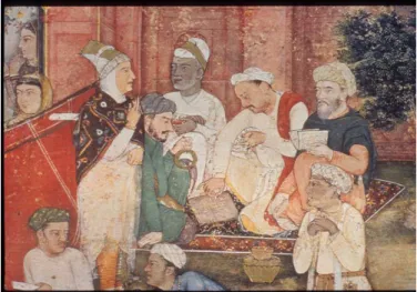
According to Professor Sreeramula Rajeswara Sarma,¹⁰ in the following illustration, Kṛṣṇa might be the astrologer in the centre of this miniature, seated between two Muslim astrologers, and casting a horoscope for the birth of Salim, the future emperor Jahāngir. e painting is in the Museum of Fine Arts, Boston (courtesy of Pr. Sreeramula Rajeswara Sarma).
Date conversion was done using Michio Yano’s pancanga program.
¹⁰“Astronomical Instruments in Mughal Miniatures” in Studien in Indologie und Iranistik 16-17 (1992) 235-276. Reprinted in e Araic and the Exotic: Studies in the History of Indian Astronomical Instruments, Manohar, New Delhi 2008.
Figure 1: Kṛṣṇadaivajña¹¹
e word upapatti
is word is used by commentators when they want to give an explanation or a justication of a rule given in the work they are commenting upon. In mathematical texts, rather than a full demonstration such as we may know nowadays, this word indicates that the operation or the procedure formulated by the author is coherent and achieves the result which it has been created for.
Here Kṛṣṇadaivajña justies the cakaravāla rule by showing why the use of the kuṭṭaka is necessary to nd integral solutions of a Pell’s equation.
Notations for operations
To support his reasoning he makes some calculations and uses formal notations. Here is a page of a manuscript with an example of these notations.
Figure 2: A manuscript page of the Bījapallava
We can read on lines 3 to 5 (we have supplied between square brackets some words or signs which are missing but which can be found in other manuscripts):
¹¹“Astrologers casting the Horoscope,” detail from the “Birth of Salim,” Museum of Fine Arts, Boston, 17.3112. Cf. Stuart Cary Welch, Imperial Mughal Painting, London 1978, Pl. 16, pp. 70-71.
tatra pūrvakaniṣṭaṃ i • ka 1 kṣe
asya vargaḥ iva • kava kṣeva 1
prakṛtiguṇaḥ iva • kava • pra 1 kṣeva 1
jyeṣṭhasādhārthaṃ kṣepaś cā-yaṃ[iva 1
kṣe 1 ]
atha kṣepabhaktajyeṣṭhādhikaṃ [kaniṣṭhaṃ] i • ka 1 jye 1 kṣe [1]
asya vargaḥ iva • kava [1] i • ka [•] jye [2] jye[va] 1 [kṣeva 1]
pra-kṛtiguṇaḥ pra • i[va •] kava 1 [pra •] i [•] ka [•] jye 2 pra [•] jyeva 1
kṣeva [1]
e explanation of this system is as follows: It uses the rst syllable of a word as algebraic symbols: i stands for iṣṭa (assumed number), ka for kaniṣṭha (least root), jye is jyeṣṭha (greatest root), pra for prakṛti and kṣe for kṣepa (additive). e Sanskrit word for square is varga, so to denote the square of one quantity, the syllable va is postponed to the syllable representing the quantity: kava means the square of the kaniṣṭha, x2.
A bullet is a multiplication sign, but not in all manuscripts. Fractions are noted by puing the numerator above the denominator, without any fraction line. ere is no sign for addition, only a number is placed aer a symbol as a counting indication; for instance if we want to note the square of the sum of the least (ka) and greatest roots (jye), it will be wrien like this: kava 1 ka•jye 2 jyeva 1 (x2+ 2xy + y2).
Finally the calculations are separated from the text by a frame. Here is the translation of this passage:
Now, the preceding least root is αx
k ; its square α2x2
k2 multiplied by the prakṛti is: α2x2p
k2 and, in order to calculate the greatest root, the additive is this one: [
α2 k
] . en, [the least root], added to the greatest one divided by the additive is: αx+ y
k ;
its square,α2x2+ 2αx y + y2
k2 , multiplied by the prakṛti is:
pα2x2+ 2pαx y + py2
k2 .
A preliminary study
As a starting point to his justication, Kṛṣṇa mentions the rule for the additive simplication by a square: “If the additive is divided by the square of an assumed number…” (see page 7) and he uses it twice: First in the ‘multiplicative form’, multiplying the least root by an arbitrary number, he says that the additive must be multiplied by the square of that number. If we denote αthe arbitrary number and if we have a triple [x1, y1; k1], we have a newleast root αx1and a
new additive α2k1.
en he uses the same rule, choosing as assumed number the additive of the triple and dividing the just obtained least root and additive. Doing this, he concludes that we have again a new least root and additive:
x2= αx1 k1 k2 = α2k1 k12 = α2 k1 And he remarks:
“In these conditions, one must imagine a number chosen in this way: Once the least root is multiplied by this number, there will be a simplication if it is divided by the additive, if not how could the least root be non-fractional?
For this purpose —that is to say: What is the number by which the least root being multiplied then divided by the additive will be without remainder?— a multiplier
and a quotient must be calculated aer making the least root a dividend, the additive a divisor without any k-additive.¹²”
Indeed, if we want x2 to be an integer we must choose α such that k1 divides αx1 so, we
must solve the following kuṭṭaka:
x1u= k1v
And Kṛṣṇa concludes:
“In that case, the quotient will be the least root. e square of the multiplier —the very [number] sought, which is the multiplier in this [kuṭṭaka]— divided by the previous additive will be the additive. en, the greatest root multiplied by the multiplier and divided by the additive will be the greatest root.¹³”
If the couple (α, β) is a solution of the kuṭṭaka x1u= k1v, the quotient is β = αx1
k1 and we
recognise the value calculated above by Kṛṣṇa as the new least root, x2; the associated values
for the additive, k2, and the greatest root, y2, follow. From the general solution of this kuṭṭaka
without k-additive, namely: u = k1t, v = x1twith t an arbitrary integer, we can see that
the new triple [x2, y2; k2] is composed of integral values:
x2 = β = α x1 k1 = k1t x1 k1 = t x1; k2 = α2 k1 = k12t2 k1 = k1t 2; y 2 = α y1 k1 = k1t y1 k1 = t y1
Of course we recognise the ‘simplication rule’ (page 7) under its multiplicative form, but what is interesting in Kṛṣṇa’s explanation is the reason for introducing the kuṭṭaka and the distribution of the roles: e least root is a dividend and the additive a divisor. He will never explain why the greatest root is chosen as the k-additive but will show by a calculation that this choice allows the new additive to be minimised.
Explanation of Bhāskara’s rule for the cakravāla
“e master endeavoured to calculate dierently because in the [preceding calcu-lation] the additive is too large. A multiplier and a quotient are calculated puing the least root (x1) as thedividend, the greatest root (y1) as thek-additive and the
additive (k1) as thedivisor.¹ ”
e ‘preceding calculation’ is the one done by Kṛṣṇa in his preliminary study; according to it, the new additive obtained aer applying the kuṭṭaka is: k2 = α
2
k1, αbeing the multiplier of the resolved kuṭṭaka.
Of course, even if the preliminary study clearly shows how to produce integral solutions for a Pell’s equation, as the goal of the cakravāla is to produce an additive equal to ±1 or ±2 or ±4, as stated in the Bhāskara’s last rule: “If the additive is two or four …” (see page 10), and from there to use the bhāvanā as a shortcut to nd the integral solutions of p x2+ 1 = y2, in Kṛṣṇa’s study the size of the additive cannot be mastered.
Kṛṣṇa will now justify that the new additive proposed by Bhāskara, k2 = ±α 2− p
k1 , which
can be minimised by the choice of α, is the right additive, if the new least root is set to be the quotient obtained in the kuṭṭaka with k-additive xed as the previous greatest root, y1.
¹²See text 6, page 20. ¹³Text 7, page 20. ¹ See the rule page 9.
Comparing the least root in Kṛṣṇa’s study with Bhāskara’s least root Kṛṣṇa introduces his calculations like this:
“A [new] least root has been previously put as the least root multiplied by the mul-tiplier¹ and divided by the additive but now the least root multiplied by the multi-plier and added to the greatest root then divided by the additive will be a [new] least root. erefore the greatest root divided by the additive is produced as an additional [number] to the least root. us, let us see what number is added to the square of the least root multiplied by the prakṛti.¹ ”
Applying Bhāskara’s rule, let (α, β) be a solution of the kuṭṭaka: x1u+ y1 = k1v, a new
least root is β = α x1+ y1
k1 and Kṛṣṇa makes this calculation:
p(α x1+ y1 k1 )2 = p α 2x2 1+ 2 p αx1y1+ p y12 k21 = p α 2x2 1+ 2 p αx1y1+ p (p x21+ k1) k12 using y 2 1 = p x21+ k1 = p α 2x2 1+ 2 p αx1y1+ p2x21+ p k1 k21 = p(α x1 k1 )2 + 2 p αx1y1+ p 2x2 1+ p k1 k21 So, the boxed number is the sought one.
en Kṛṣṇa remarks that in his previous reasoning the square of the multiplier (α) divided by the additive has to be added in order to nd the greatest root and, for this purpose, he splits the number he has just calculated in two components:
2 p αx1y1+ p2x21+ p k1 k21 = 2 p αx1y1+ p2x21 k12 + p k1 (∗)
And now the argument is:
“With this additional number, the prakṛti divided by the additive is added, but the square of the multiplier divided by the additive must be added, thus in this [rule] the dierence between the square of the multiplier and the prakṛti divided by the additive must be also added, because doing this, only the square of the multiplier divided by the additive will be added.¹ ”
With this argument the new additive, α2− p
k1 , given by Bhāskara’s rule is now justied:
p k1 + α2− p k1 = α2 k1
since this last result will enable us to nd a greatest root if we add it to p(α x1 k1
)2
as shown in the preliminary study.
Kṛṣṇa also explains why the new additive has to be ‘reversed’ if the prakṛti is greater than the square of the multiplier, the result being the same in both cases. Let us summarise these reasons using modern notations:
¹ Calculated by the kuṭṭaka. ¹ Text 4, page 20.
if α2 ≥ p then p k1 + α2− p k1 = α2 k1 if α2 ≤ p then p k1 +( − p− α2 k1 ) = α2 k1
Putting things together
Aer this separate study about the additive according to Bhāskara’s rule, Kṛṣṇa takes into ac-count the rst member of the number (∗) he had split in two parts and says: “No doubt then that this very number, 2 p αx1y1+ p2x21
k21 , is added to the square of a greatest root, namely the square of α y1
k1 .”
To understand what is meant here, let us summarise the full calculation made by Kṛṣṇa 1. Firstly he develops p(α x1+ y1
k1
)2
and, using the identity: y12= p x21+ k1, he obtains this
equality: p(α x1+ y1 k1 )2 = p(α x1 k1 )2 + 2 p αx1y1+ p 2x2 1 k21 + p k1
2. He then adds, or subtracts, the additive given by the rule: α2− p k1 : p (α x1+ y1 k1 )2 ± α2− p k1 =p (α x1 k1 )2 +2 p αx1y1+ p 2x2 1 k12 + α2 k1
3. He adds the rst and the last terms of the second member of the equality, aer remarking that this sum is a greatest root:
p(α x1+ y1 k1 )2 ± α2− p k1 = (α y1 k1 )2 +2 p αx1y1+ p 2x2 1 k21
Now the justication of the cakravāla rule is complete because the last result is a square: (α y1 k1 )2 +2 p αx1y1+ p 2x2 1 k12 = (α y1+ p x1 k1 )2
And thus we have a new triple that veries the relation p x2
2+ k2= y22: x2 = α x1+ y1 k1 k2 = α2− p k1 y2= α y1+ p x1 k1
Kṛṣṇa concludes his upapai like this:
“When a least root multiplied by an assumed number and added to a greatest root [the result] being divided by an additive is put as a least root, then the dierence between the square of the assumed number and the prakṛti divided by the additive is an additive. e greatest root multiplied by the assumed number and added to the least root multiplied by the prakṛti, [the result] being divided by the additive is then the [new] greatest root.
In this procedure, even if there is no requirement of the kuṭṭaka —roots being ob-tained only by force of an assumed number— a kuṭṭaka is nevertheless performed for a state of non-fractionation [of the roots]; hence the statement: “Having made the least and greatest roots and the additive…¹ is justied”
e rst paragraph is a summary of Bhāskara’s rule with a slight dierence: while the rule says: “e quotient associated to the multiplier is a least root, whence a greatest root”, that is to say that once we have a least root and an additive, we can calculate the associated greatest root by the general relation: p x2+ k = y2, we can nevertheless calculate the greatest root using the result of Kṛṣṇa’s calculations: y2 = α y1+ p x1
k1 where α is a solution of the kuṭṭaka laid
down for the cakravāla.
In the second paragraph, we have an interesting observation: Whatever the number d is, if [x1, y1; k1] is a triple, solution of a Pell’s equation, [dx1, dy1; d2k1] is another such triple. Kṛṣṇa
uses this to prove that the result in the cakravāla rule is a square when he remarks that the additiveα2− p
k1 eliminates
p
k1 and that, in fact, we get a greatest root while combining p
(α x1 k1
)2 and what remains: α2
k1.
Final remarks
What Kṛṣṇa really demonstrates here is that if we follow Bhāskara’s rule, puing as a least root x2 = α x1+ y1
k1 , the quotient of a well-chosen kuṭṭaka, and as additive
α2− p k1 , the result is a square.
Another very interesting point is his aempt, in the preliminary study, to justify the use of the kuṭṭaka if we want integral solutions. e use of the full kuṭṭaka, with the greatest root as a k-additive, is not explained though, but it is certainly not obvious!
e expression found for the greatest root allows to make an iterative description of the cakravāla process: Let [x1, y1; k1] be a triple of integers such as p x12+ k1= y12and let u1and
v1be integral solutions of x1u+ y1= k1v, such that |u21− p| is minimal, then:
x2 = x1u1+ y1 k1 k2= u21− p k1 y2 = u1y1+ p x1 k1 is a new triple of integers verifying the same relation.
From there, other triples can be calculated by induction; but, as the dierence between the square of the solution of the kuṭṭaka and the prakṛti is minimised —that is to say: the additive— at each step, the process will come to an end with an additive equal to 1. is also is not obvious. A question which is not approached by Kṛṣṇa —nor by Bhāskara— is: Why is the additive, α2− p
k1 an integer? We can answer this question, supposing that the least root, x1 and the
additive, k1, are relatively prime —if they are not, the equation could be transformed into an
equation with additive equal to 1, and the cakravāla is useless in that case. We multiply α2− p by x21and obtain the following identities:
(α2− p) x21 = α2x21− p x21
= α2x21− y21+ k1 (because p x21 = y21− k1)
= (α x1+ y1)(α x1− y1) + k1
en k1 divides the right member of the last identity, because α had been chosen for this
purpose, so k1must divide the le member and as it does not divide x1, it must divide α2− p.
e last remark we can make is: How has such a sophisticated method been developed? e answer might be found in some unknown works or commentaries in the multitude of manuscripts stored in libraries in India.
5 Examples
Bhāskara puts forward examples in order to illustrate the theoretical part of the cakravāla. He asks to solve these two equations:
67 x2+ 1 = y2 and 61 x2+ 1 = y2
We give briey the solutions according to Kṛṣṇa’s commentary but using our modern no-tations (starred items indicate the beginning of a cycle).
67 x2+ 1 = y2
*1. Choose a suitable triple: [x1, y1; k1] = [1, 8; −3] 67 × 12− 3 = 82
2. Solve the kuṭṭaka: u+ 8 = −3 v : u0= 1 v0 = −3
3. Calculate p− u20 = 67 − 1 = 66
4. Calculate p− u20 = 67 − 1 = 66 e result is not small.
5. Other solutions of the kuṭṭaka are: u = 1 − 3t v = −3 + t. Choose t = −2 : u1 = u0− 2 × −3 = 7 v1 = −3 − 2 = −5
6. Calculate p − u21= 67 − 49 = 18 which minimises the dierence.
e additive is: k2 = −p− u
2 1
k1 = −
18 −3 = 6 e least root is: x2 = v1= −5
e greatest root is: y2 = 41
*7. A new triple is: [x2, y2; k2] = [5, 41; 6] e new vargaprakṛti is: 67 x2+ 6 = y2
8. Solve the kuṭṭaka: 5 u + 41 = 6 v : u0 = 5 v0 = 11 9. Calculate p− u20 = 67 − 25 = 42
e additive is: k3 = −p− u 2 0
k2 = −
42 6 = −7 e least root is: x3 = v0= 11
e greatest root is: y3 = 90
*10. A new triple is: [x3, y3; k3] = [11, 90; −7] e new vargaprakṛti is: 67 x2− 7 = y2
11. Solve the kuṭṭaka: 11 u + 90 = −7 v : u0 = 9 v0 = −27
12. Calculate u20− p = 81 − 67 = 14 e additive is: k4 = u
2 0− p
k3 =
14
−7 = −2
e least root is: x4 = −27
e greatest root is: y4 = 221 67 × 272− 2 = 2212
*13. A new triple is: [x4, y4; k4] = [27, 221; −2] e new vargaprakṛti is: 67 x2− 2 = y2
14. e additive is now −2 and we can use the bhāvanā as a shortcut: 27 221 −2
27 221 −2
e least root is: x5 = 2 × 27 × 221 = 11934
e greatest root is: y5 = 67 × 272+ 2212 = 97684 e additive is: k5 = (−2)2= 4
15. e additive being a square, we can now use the simplication rule, dividing k5by 4 we
have to divide the roots by 2 and nd the solution: 67 × 59672+ 1 = 488422
e second example is more impressive and uses fractional intermediary roots. 61 x2+ 1 = y2.
*1. Choose a suitable triple: [x1, y1; k1] = [1, 8; 3] 61 × 12+ 3 = 82
2. Solve the kuṭṭaka: u+ 8 = 3 v : u0 = 1 v0 = 3 and, as in the previous example,
choose other solutions u1= 1 + 2 × 3 = 7 v1 = 3 + 2 = 5, which minimises p − u21
3. Calculate p − u21= 61 − 49 = 12
e additive is: k2 = −p− u
2 1
k1 = −
12 3 = 4 e least root is: x2 = v1= 5
e greatest root is: y2 = 39
*4. A new triple is: [x2, y2; k2] = [5, 39; −4] e new vargaprakṛti is: 61 x2− 4 = y2
5. e additive being a square, we can now use the simplication rule, dividing k2 by 4
we have to divide the roots by 2 and nd fractional solutions with triple: [x3, y3; k3] =
[5 2,
39 2; −1]
6. Using an equal bhāvanā, we get a new triple: [x3, y3; k3] = [1952 , 15232 ; 1]
7. Compose this triple with the preceding one and obtain the triple: [x4, y4; k4] = [3805, 29718 ; −1]
8. An equal bhāvanā yields the solution:
61 × 2261539802+ 1 = 17663190492
Sanskrit texts
Text 1.
vargaḥ prakṛtir yatreti vargaprakṛtiḥ yato 'sya gaṇitasya yāvadādivargaḥ prakṛtiḥ yadvā yā-vadādivargeṣu prakṛtibhūtād aṅkād idaṃ gaṇitaṃ pravartata iti vargaprakṛtiḥ atra yāvadva-rgādiṣu prakṛtibhūto yo 'ṅkaḥ sa prakṛtiśabdenocyate sa cāvyaktavargaguṇaka eva ato 'tra padasādhane vargasya yo guṇaḥ sa prakṛtiśabdena vyavahṛyate
Text 2.
evaṃ cakravālena caturdvyekayutau catuḥkṣepe dvikṣepa ekakṣepe cābhinne pade bhavataḥ idam upalakṣaṇam yatra kutrāpi kṣepe 'bhinne pade bhavataḥ yutāv ity apy upalakṣanam tena śuddhāv apīti jñeyam
Text 3.
atha rūpakṣepapadānayane prakārāntaram apy astīty āha ``caturdvikṣepamūlābhyām'' iti catuḥkṣepamūlābhyāṃ dvikṣepamūlābhyāṃ ca rūpakṣepārthaṃ bhāvanā rūpakṣepārthabhā-vanā kāryeti śeṣaḥ catuḥkṣepe ``iṣṭavargahṛtaḥ kṣepa'' ityādinā dvikṣepe tu tulyabhāvanayā
catuḥkṣepapade prasādhya paścād ``iṣṭavargahṛtaḥ kṣepa'' ityādinā rūpakṣepaje pade vā bha-vata itiyarthaḥ
Text 4.
pūrvaṃ tu guṇaguṇitaṃ kaniṣṭhaṃ kṣepabhaktaṃ sat kaniṣṭhaṃ bhavatīti sthitam idānīṃ tu guṇaguṇitaṃ kaniṣṭhaṃ jyeṣṭhayutaṃ kṣepabhaktaṃ sat kaniṣṭhaṃ syāt tasmād jyeṣṭhaṃ kṣe-pabhaktaṃ kaniṣṭhe 'dhikaṃ jātam evaṃ sati prakṛtiguṇe kaniṣṭhavarge kim adhikaṃ bhavatīti vicāryate
Text 5.
caturadhike antyapadakṛtis tryūnā dalitā antyapadaguṇā antyapadam antyapadakṛtis vyekā dvihṛtā ādyapadāhatā ādyapadam
caturūne antyapadakṛtī tryekayute vadhadalam pṛthak vyekam vyekāḍyāhatam antyam padavadhaguṇam ādyam āntyapadam Text 6.
atreṣṭaṃ tādṛśaṃ kalpanīyaṃ yena guṇitaṃ kaniṣṭhaṃ kṣepabhaktaṃ śuddhyet anyathā kani-ṣṭham abhinnaṃ kathaṃ syāt
tadarthaṃ kaniṣṭhaṃ kena guṇitaṃ kṣepabhaktaṃ niḥśeṣaṃ syād iti kaniṣṭhaṃ bhājyaṃ pra-kalpya kṣepaṃ haraṃ ca prapra-kalpya kṣepābhāve guṇāptī sādhye
Text 7.
atra yā labdhis tat kaniṣṭhaṃ padam yo 'tra guṇas tad eveṣṭam iti guṇakavargaḥ pūrvakṣepa-bhaktaḥ kṣepaḥ syāt jyeṣṭham api guṇaguṇitaṃ kṣepabhaktaṃ jyeṣṭhaṃ syāt
Text 8.
anenādhikena kṣepabhaktā prakṛtiḥ kṣiptā syāt kṣepaṇīyas tu kṣepabhakto guṇavargaḥ tad atra guṇavargaprakṛtyor antarālam api kṣepabhaktaṃ kṣepyam tathā sati kṣepabhakto guṇavarga eva kṣipto bhavet
Text 9.
yadā tv iṣṭaguṇaṃ kaniṣṭaṃ jyeṣṭhayutaṃ kṣepabhaktaṃ sat kaniṣṭhaṃ kalpyate tadā guṇa-vargaprakṛtyor antaraṃ kṣepabhaktaṃ sat kṣepo bhavatīṣṭaguṇaṃ jyeṣṭhaṃ prakṛtiguṇakani-ṣṭena yutaṃ kṣepabhaktaṃ sat tatra jyeṣṭhaṃ bhavatīti
atra yady apy iṣṭavaśād eva padasiddhir astīti kuṭṭakasya nāpekṣā tathāpy abhinnatvārthaṃ kuṭṭakaḥ kṛtaḥ ata upapannaṃ hrasvajyeṣṭhapadakṣepān ityādi
References
[1] André Weil, Number eory, An approa through history from Hammurapi to Legendre, Reprint of the 1984 Edition, Birkhäuser, Boston, 2007
[2] Clas-Olof Selenius, Rationale of the akravāla process of Jayadeva and Bhāskara II, in His-toria Mathematica 2, 1975 pp 167-184
[3] Kṛṣṇadaivajña, Bīja Pallavam a commentary on Bīja Ganita, the Algebra in Sanskrit, Edited with Introduction by T.V. Radhakrishna Sastri, Tanjore Saraswati Mahal Series N° 78, Tan-jore, 1958
[4] A. A. Krishnaswami Ayyangar, New Light on Bhaskara’s Chakravala or Cyclic Method of solving Indeterminate Equation of the Second Degree in Two Variables, Journal of the Indian Mathematical Society, 1929-30, Vol.18
[5] Edward Evere Whitford, e Pell Equation, College of the city of New York, 1912 [6] Edward Strachey, Bija Ganita or the Algebra of the Hindus, London, 1813(partly translated
from a Persian translation by Ata Alla Rasheedee in 1634)
Manuscripts
[1] Bījapallava, Bhandarkar Oriental Institute, Puṇe, No 287 of Viśrāma (1), foll. 133 [2] Bījapallava, Bhandarkar Oriental Institute, Puṇe, No 538 of 1895-1902, foll. 116 [3] Bījapallava, Maharaja Maan Singh Pustak Prakash Research Center, Jodhpur, foll. 243