HAL Id: hal-03023595
https://hal.archives-ouvertes.fr/hal-03023595
Submitted on 25 Nov 2020
HAL is a multi-disciplinary open access
archive for the deposit and dissemination of
sci-entific research documents, whether they are
pub-lished or not. The documents may come from
teaching and research institutions in France or
abroad, or from public or private research centers.
L’archive ouverte pluridisciplinaire HAL, est
destinée au dépôt et à la diffusion de documents
scientifiques de niveau recherche, publiés ou non,
émanant des établissements d’enseignement et de
recherche français ou étrangers, des laboratoires
publics ou privés.
Beam size dependency of a laser-induced plasma in
confined regime: Shortening of the plasma release.
Influence on pressure and thermal loading
Alexandre Rondepierre, Selen Ünaldi, Yann Rouchausse, Laurent Videau,
Rémy Fabbro, Olivier Casagrande, Christophe Simon-Boisson, Hervé
Besaucéle, Olivier Castelnau, Laurent Berthe
To cite this version:
Alexandre Rondepierre, Selen Ünaldi, Yann Rouchausse, Laurent Videau, Rémy Fabbro, et al..
Beam size dependency of a laser-induced plasma in confined regime: Shortening of the plasma
re-lease. Influence on pressure and thermal loading. Optics and Laser Technology, Elsevier, 2021, 135,
�10.1016/j.optlastec.2020.106689�. �hal-03023595�
Beam size dependency of a laser-induced plasma in confined regime:
Shortening of the plasma release. Influence on pressure and
thermal loading
Alexandre Rondepierre
a,b,*, Selen Ünaldi
a, Yann Rouchausse
a, Laurent Videau
c,d,
R´emy Fabbro
a, Olivier Casagrande
b, Christophe Simon-Boisson
b, Herv´e Besauc´ele
b,
Olivier Castelnau
a,*, Laurent Berthe
a,*aLaboratoire Proc´ed´es et Ing´enierie en M´ecanique et Mat´eriaux (PIMM), UMR8006 ENSAM, CNRS, CNAM, 151 bd de l’Hˆopital, 75013 Paris, France bTHALES LAS France, 78990 Elancourt, France
cCEA, DAM, DIF, 91297 Arpajon, France
dUniversit´e Paris-Saclay, CEA, Laboratoire Mati´ere en Conditions Extrˆemes, 91680 Bruy´eres-le-Chˆatel, France
Keywords:
Plasma release Plasma lifetime Laser shock peening Thermal effect VISAR analysis Finite element method
A B S T R A C T
Processes using laser-shock applications, such as Laser Shock Peening or Laser Stripping require a deep under-standing of both mechanical and thermal loading applied. We hereby present new experimental measurements of the plasma pressure release regarding its initial dimension, which depends on the laser beam size. Our data were obtained through shock waves’ velocity analysis and radiometric assessments. A new model to describe the adiabatic release behavior of a laser-induced plasma with a dependency to the beam size is developed. The results and the associated model exhibit that the plasma release duration is shortened with smaller laser spots. As a consequence, with chosen smaller laser spots (0.6 mm to 1 mm), the thermal loading applied during the plasma lifetime will also decrease. These new results shall help for a better understanding of laser-matter interaction for laser-shock applications by giving more accurate plasma profiles. Thus, process simulations can be improved as well. Eventually, by considering recent developments with high-power Diode Pumped Solid-State lasers (DPSS), we now expect to develop a new configuration for LSP which could be applicable both without any thermal coating and deliverable by an optical fiber.
1. Introduction
Laser-induced plasma consists in a high-power pulsed laser (1 J, 10 ns) focused on a metal target in order to vaporize and ionize it. A plasma is then rapidly created, and the remaining laser energy is used to heat the formed plasma and increase its pressure. As a reaction of this high- pressure generated by the plasma, shock waves propagate inside the material.
Laser Shock Applications, which rely on the generation of a high- pressure plasma, are in development for last 60 years, since the exper-imental discovery of laser by Maiman in 1960. Among these applica-tions, we can find Laser Shock Peening (LSP), LAser Shock Adhesion Test (LASAT, [1]) and Laser Stripping (LS, [2]). LSP is a laser shock process that is similar to shot peening and applied in many fields such as
aeronautics and nuclear power plants [3,4]. Shock waves, which prop-agate inside the material, lead to deformations, and deep compressive residual stresses (CRS) are generated up to more than 1 mm, for aluminium alloy for example. On the other hand, for a conventional shot peening, the depth of the generated CRS is around 0.25 mm [5]. These CRS help to enhance fatigue life of the treated material by retarding the crack initiation and slowing down its propagation [6]. Furthermore, it can also improve the resistance against pitting corrosion [7].
The confined regime was developed in 1970 as, initially, both the pressure and the duration of the plasma were quite low. Anderholm [8]
demonstrated that one can significantly increase the pressure magnitude by 4 times higher than in direct regime, at the same power density, and by 2 times its duration. This can be done by confining the plasma with a medium transparent to the laser wavelength, such as water, quartz or
* Corresponding authors at: Laboratoire Proc´ed´es et Ing´enierie en M´ecanique et Mat´eriaux (PIMM), UMR8006 ENSAM, CNRS, CNAM, 151 bd de l’Hˆopital, 75013 Paris, France (A. Rondepierre).
2. Experimental setup and used methods 2.1. Hephaistos laser facility and optical setup
Experiments presented in this paper were performed at the Hephaïstos laser facility, located in the PIMM laboratory (Proc´ed´es et Ing´eni´erie en M´ecanique et Mat´eriaux). It consists in a Thales Gaïa HP laser, which is a flashlamp-pumped Nd:YAG laser (2*7 J, 7.2 ns, 2 Hz, @532 nm).
The beam is focused with a 350 mm converging lens to obtain desired focal spots. These spots were precisely measured through an imaging setup via camera, with a magnification of 10. The used spot sizes were: 3 mm, 2 mm, 1.5 mm, 1 mm, 0.8 mm and 0.6 mm. Energies were measured for each case with a Gentec-EO calorimeter.
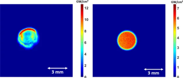
In the case of large spots (>3 mm), as our laser spot experiences over- intensities due to diffraction effects and long-distance propagation, the beam was spatially smoothened thanks to the use of a DOE (Diffractive Optical Element) as shown on Fig. 1. It is important to ensure the uni-formity of intensity’s distribution for large spots as we used the mono-dimensional assumption for the plasma release.
Furthermore, the laser pulse duration was measured with a DET10A2 (Thorlabs) photodiode. Temporal profile is represented on Fig. 2.
Finally, we used power densities ranging from 1 to 4 GW/cm2, to
avoid laser breakdown plasma inside the confinement (threshold: 8 GW/ cm2, [21]).
2.2. Plasma lifetime measurements with high-speed photodiode
The plasma lifetime was measured by using an optical setup (see
Fig. 3). To do this, the radiant intensity emitted by the plasma is temporally acquired. For this purpose, we used an afocal system and we ensured that the whole plasma was at each time captured by the photodiode. Two converging lenses were used, one of +200 mm focal length and one of +80 mm length which was the closer to the plasma. In this case, the numerical aperture of the system is high and hence we have an optimized intensity signal.
Measurements were done with a fast photodiode (FND-100Q from Excelitas) with an optical notch filter at @532 nm and a band-pass filter (@800–840 nm) to not be disturbed by the laser pulse emission. As we consider the plasma as an ideal gas, thus the pressure could be easily related to the temperature.
With this optical setup, we can measure the radiant intensity, abusively called intensity. This light emission is directly depending on the temperature, through Planck’s law, and so it is also directly related to the pressure.
From Planck’s law, we can calculate the radiance LΩ by making an
integer in the range of our filter. As the geometry is fixed for our setup, the radiance (W⋅sr−1⋅ m−2) can directly be linked with the radiant flux
(W), which was measured by our photodiode.
LΩ(t) =
∫840nm
800nm
2hc2
λ5eλkBT(t)hc − 1dλ (1)
λ is the wavelength, kB the constant of Boltzmann, h the constant of
Planck and c the speed of light. T is the plasma temperature that can be obtained with the ideal gas law:
T(t) =P(t)V(t)
nRm (2)
Rm being the ideal gas constant and n the chemical amount, assumed
constant after laser ablation. Finally, the radiant intensity can be calculated and normalized to be compared with experimental (and also normalized) intensity measured with the photodiode.
solid polymers [9] which allows to operate with low energy lasers. Today, all industrial applications are used in the confined regime. Furthermore, these applications also need a thermal coating to be applied before laser shots in order to protect the metal from thermal damage, as the plasma reaches temperature of more than 10 000 K [10]. However, at end of the 90’s, Sano et al. have been developing LSP without thermal Coating (LPSwC), by using small focal spot sizes, up to 0.6 mm compare to more than 5 mm for other applications with the thermal coating [11]. On the other hand, laser systems based on DPSS lasers delivering high energy (up to 1 J) at high-frequency (up to 200 Hz), are now available. These lasers could be delivered through an op-tical fiber and used with small focal spots without impacting the treat-ment time compared with the configuration with thermal coating. Indeed, in that case large spot sizes are used and it requires lasers of more than 10 J, which are limited to a repetition rate of 10 Hz.
Yet, in the LSPwC configuration, some thermal damages can occur and the surface will experience oxidation [12]. In addition, both roughness and stress measurements made between large and small focal spot configurations are greatly different [13].
Then, we expect the first layers of the treated samples to be under tensile stresses, which are detrimental for fatigue issues and compromise the positive effect of LSP.
Hence, it is crucial to correctly understand the laser-induced plasma behavior for simulations and process optimizations. Previous works [14]
have already developed analytical models for the plasma behavior (loading and releasing), in the range of large focal spots (4 mm to 10 mm), where models can be simplified into a monodimensional case. Most recently, numerical models were developed [15] and show a good agreement with the existing analytical model [16,17]. Simulations of LSP process are in great development. However recent simulation works tend to configuration using small spot size (from 1 mm to 3 mm) but implement pressure loading profile developed for large and mono-dimensional spot [18,19].
However, previous models developed for large spots are no longer valid for small focal spots as the monodimensional assumptions cannot be done anymore. Indeed, as smaller the spot size will be, as greater the relative radial leaking release of the plasma will be, and hence it should be taken into account.
Moreover, it is also well-known that the release of the plasma is drastically reduced at longer time (more than 1 μs) when using
sub-millimeter laser spots [20].
Then, we are here interested in the physical comprehension of these different configurations, necessarily leading to different plasma profiles regarding the focal spot size. Thus, it is very important to know the plasma behavior, and especially its duration which drives the thermal loading, as high-temperature can induce detrimental effects such as tensile stresses inside the metal, which attenuate the positive effect of the LSP treatment.
This paper presents new results for the plasma pressure release, and highlights the changes in the plasma behavior as a function of laser spot size. These results have been obtained with plasma-induced shock waves’ velocity profile (which lies with the plasma pressure loading), but also through the plasma lifetime, which was obtained with radiant intensity measurements, with a high-speed photodiode. Moreover, a Radius dependent Model (RM) has been developed in order to under-stand and validate new experimental results.
In a first part, the used experimental setup will be described, and secondly we will present our new experimental results about the plasma release. Then, we will introduce how the release, with a dependency to the laser beam size, can be modeled in a good accordance with experi-mental results. Finally, we will analyze what will be the influence of using small spots sizes, regarding mechanical and thermal loading, for laser shock processes.
2.3. Shock waves velocity measurement by VISAR (Velocity Interferometer System for Any Reflector)
An effective method for determining the pressure generated by the laser as function of its intensity (in GW/cm2) is to measure the velocity
of the induced shock wave.
We measured the pressure induced by the plasma using a VISAR (see
Fig. 3), which is based on a Barker one [22,23]. A VISAR is a very
accurate optical tool, for time-resolved velocity measurements, consti-tuted of two parts: a probe laser (Coherent, VERDI 1 W CW @532 nm), focused on the rear-surface of the target, that will be wavelength-shifted by Doppler effect, and a Michelson type interferometer to measure the Doppler shift and link it to the rear velocity.
2.3.1. Use of BK7 glass plate
When using small focal spots, one should be careful about what is called edge effects [24–26]. These mechanical effects are coming from the fact that there is a huge discontinuity of pressure between the laser spot area (going up to several GPa), and the outside of this area (expe-riencing almost no pressure). Hence, release waves coming from the edge of the focal spot (where there is a discontinuity of pressure) propagate towards the center of the laser spot. Moreover, as these release waves propagate faster than shock waves, they will catch shock waves and modify their amplitudes and durations: shock waves are attenuated. This catch will occur in smaller depths when using smaller laser spots. Thus, in order to avoid measuring a wrong profile for shock waves (linked to plasma pressure profiles) we have to use very thin foils of aluminium. However, in this case, the back-and-forth propagation of shock waves inside the aluminium is too fast, and it interferes with the release of the main shock wave. In addition, due to the use of small spot diameter, strong deformation of target and laser probe deflection will arise.
In order to avoid these issues, the aluminum target is stuck with a BK7 glass plate which has the same mechanical impedance as shown in
Table 1. The bounding between the Al-foil and the BK7 glass is made with a very thin layer (a few μm) of a commercial glue (ethyl
2-cyano-acrylate). Therefore, the shock wave will propagate inside the BK7 with no reflection and the aluminium surface will not undergo defor-mation. As BK7 is transparent to green wavelength, the material velocity at the interface between aluminium and BK7 is measured with VISAR.
To ensure that this method was correct, we compared on Fig. 4 the velocity profiles with a spot size of 3 mm and an aluminium foil of 0.3 mm with and without BK7 glass plate.
The second peak, only visible without BK7, corresponds to the back- and-forth of the shock waves inside the material, as it is reflected at the
Fig. 1. Spatial distribution of intensity (Imean=4 GW/cm2) with DOE (right) and without DOE (left) for a 3 mm laser spot size.
Fig. 2. Temporal profile of the laser pulse (FWHM = 7.2 ns).
Fig. 3. Imaging setup used.
Table 1 Material parameters. Material σy (GPa) (GPa) E ρ (g/cm3) ν Z (g/cm2s) C (m/ s) Aluminium 0.120 69 2750 0.33 1.38.106 6328 BK7 0.64 82 2460 0.206 1.42.106 5640
interface between aluminium and air while there is clearly no reflection at the interface between aluminium and BK7.
2.3.2. Simulations
The plasma behavior cannot be directly deduced from velocity measurements as shock waves will spread and attenuate during propa-gation. For this purpose, an Abaqus FE model (using Jonhson-Cook, see parameters in Table 2) in 2D axisymmetric was previously developed in
[9] to reproduce rear-free surface velocities and material velocities (output), and to compare them with VISAR velocity profiles. This model enables us to find the pressure profiles (input) associated with the experimental velocities.
The aim is to use as input, in Abaqus, the plasma pressure profile obtained through the new model that we have developed, and that will be presented in part 4 of this paper. Then, we checked that the simulated velocities are in good agreement with experimental results, thus con-firming the validity of the model.
For the target geometry, we used a 300 μm thickness aluminium
stuck to a 1.7 mm BK7 glass. We then calculate the temporal material velocity at the interface between aluminium and BK7, where VISAR measurements were performed, to compare it with experimental results. We finally applied the spatial profile of our laser (intensity) to reproduce the pressure loading (slowly decreasing on the edges of the laser spot), as shown on Fig. 5.
3. Results and discussions
In this part, results from a direct measurement of the plasma are presented (radiant intensity). This first diagnosis is made on the front side of the target which is hit by the laser pulse, and so where the plasma is located.
We also present results from velocity measurements, which are in-direct measurement of the plasma as velocities are obtained on the rear surface of the target. As a consequence, the behavior is quite different and numerical simulations must be used to understand whether the
profile is modified from the plasma behavior itself or from geometrical reasons, as the shock waves propagates inside the material.
3.1. Radiant intensity and plasma lifetime
Comparison between experimental intensity signals and the simu-lated intensity (calcusimu-lated using the RM model, presented on part 4) are plotted on Fig. 6. We have normalized both the signals as only the global shape (and the release duration) is mattering there; but one should note that the photodiode is calculating a radiant intensity while our simula-tion only gives us the radiance, one to the other are bound with geometrical consideration (a constant) but not identically the same.
Signals can be separated in two physical parts: the first part of the curve where the signal is rising fast corresponds to the plasma creation and heating, during the laser pulse. This part is, considering our short pulse duration, independent of the spot size and we can see that all the signals are increasing in the same way. On the other hand, the second part, corresponding to the plasma adiabatic release, shows important differences regarding the spot size. Indeed, as smaller the spot size will be as faster the release will occur. For example, it took 24 ns for a 0.6 mm spot size to decrease its intensity by 80%, while it is 47 ns for a 3 mm spot size.
These measurements were highly reproducible. Hence this experi-ment clearly shows that the temporal behavior of the plasma (here, its temperature) is dependent on the used laser focal spot.
3.2. Velocity profile
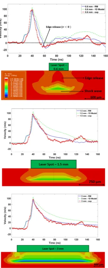
Experimental velocity profiles are plotted on Fig. 7 for 3 spot sizes: 0.6 mm, 1 mm and 3 mm. These results highlight that the loading duration, as the maximum velocity reached (related to the maximum pressure of the plasma), are independent of the spot size. But, most of all, one can see that there is a great dependency of the release duration with the laser spot size. Indeed, the release duration is shortened with smaller spot sizes.
However, as previously explained ([24]), even if we took thin plates of aluminium, there are some edge effects which are more important with smaller spots. We must then use numerical simulations with adapted geometry to separate the edge effects from the plasma pressure profile itself.
On Fig. 8, we have plotted the experimental velocity profiles
Fig. 4. Normalized velocity profile with and without BK7 for a 3 mm spot size and a 300 μm Al-foil at 1 GW/cm2.
Table 2
Johnson–Cook parameters used for aluminium.
B (GPa) C n ∊0
obtained, but also the simulated velocities from Abaqus. For simula-tions, we used a 1D-profile, obtained from Esther Code (CEA, [15]) for a 7.2 ns gaussian pulse. We then used this same profile, but with different
duration for the pressure release to show that velocity profiles can be better reproduced with a shortened pressure profile than with the 1D- model. Even though edge effects can explain the reduction in the
Fig. 5. Geometry, material and pressure profile used on Abaqus.
Fig. 6. Normalized radiant intensity comparison between experimental data and the presented model at 4 GW/cm2 (0.6 mm; 1 mm; 3 mm).
global shape of velocity profiles, it remains inaccurate and a shortening of the pressure release must be added to reproduce as good as possible the experimental profiles.
The used pressure profiles as input for Abaqus (0.6 mm, 1 mm, 3 mm and a 1D pressure model) are plotted on Fig. 9. When reducing the spot size, the release duration of the plasma has to be shortened in order to correctly reproduce velocity profiles.
One should notice that the behavior of the release was changed after a time t = 2.5τ, which corresponds to the end of the laser pulse. This
choice has been made to be consistent with the model that will be developed in part 4. Finally, we can see that, similarly to radiant in-tensity measurements, experimental results indicate that the behavior of the plasma depends on the laser spot size: its release duration will be shortened with smaller laser spots.
Fig. 8 also presents stresses mapping obtained from Abaqus. Tensile stresses go towards red color, while compressive stresses go towards blue ones. We can clearly identify whether the shock is affected or not by edge effects. Indeed, the shock waves seems to be purely plane for the 3 mm spot size compare to the 0.6 mm case, where the release of the shock waves is being attenuated by bi-dimensional effects (tensile stresses) which come from the edges and converge to the center. This is also confirmed by velocity profiles where we can clearly see a negative ve-locity at 60 ns, for the 0.6 mm spot size, due to these release waves coming from the edges.
4. Development of a spot size dependent plasma release model
We hereby present a new model to describe the laser-induced plasma pressure release in confined regime. The first part of the pressure profile (Fig. 10(b)) corresponds to the creation and heating of the plasma, during the laser pulse. This part is calculated from previous work ([14]) and will be used for the second part. One can note that we do not apply our model to the loading part as the dependency to the spot size is limited considering our used pulse durations. Then, the second part corresponds to a slow release and cooling of the plasma (it is said to be adiabatic) and will be described by our model. Previous work [14] made some assumptions to simplify the calculation of this release; it was then only valid for large spot sizes (5–10 mm). The presented model has the aim of modeling and calculating this release for any spot sizes. Finally, after the adiabatic release (≈ 1μs) and because of a rarefaction wave, a
spherical blast wave makes the pressure to rapidly decrease. This last part is also described from previous work.
4.1. Previous work: Monodimensional model
Based on the previous work from Fabbro (1990, [14]) in confined regime, we will start by describing the first part of the laser-matter interaction during which the laser is absorbed and used to heat the plasma. Then, we will describe the cooling phase assuming a mono-dimensional geometry (Fig. 10(a)). In this model, the confinement has an important effect regarding the plasma pressure duration as the confinement retains the plasma to the surface.
The temporal behavior of a laser-induced plasma under vacuum or without any confinement has already been greatly studied and modeled with Laser Supported Detonation (LSD) wave. Pirri ([20,27]) explained some scaling law regarding the plasma expansion with two separated
Fig. 8. Comparison of the experimental velocity with Abaqus simulations for
different pressure profiles (see Fig. 9), and stress map captured from Abaqus at t = 60 ns (Top:0.6 mm – Middle:1.5 mm – Bottom:3 mm).
Fig. 9. Plasma pressure profile obtained to reproduce velocity profiles on
Abaqus, at 4 GW/cm2 and for different cases (0.6 mm; 1 mm; 3 mm and 1D-case).
regimes that are axial and radial blast waves.
4.1.1. Pressure loading through laser absorption
The basic geometry of this problem in a monodimensional (1D) case is shown in Fig. 10. As the confining medium is (almost) transparent to the laser, the absorption surface is located at the boundary between the metal surface and the confinement. In this model, two shock waves of the same pressure (the plasma pressure) propagate inside the metal target and the confinement, thus tending to separate the two layers. Assuming a 1D model implies that the opening L(t) of the plasma along the laser direction is some order of magnitude smaller than the radius of the laser spot.
Basic equations for this problem are the following ones: The plasma’s opening:
dL(t)
dt =U1(t) + U2(t) (3)
where U1 and U2 are respectively the material velocities at plasma-
confinement and plasma-metal interfaces.
Rankine-Huguoniot equation for momentum conservation:
P =ρ1D1U1=ρ2D2U2=Z2U2 (4)
where Pi is the plasma pressure, ρi is the density, Di the shock velocity
and Zi the shock impedance, with 1 and 2 being respectively associated
to the metal and to the confinement. Thus ((3) and (4)): dL(t) dt = 2P(t) Z (5) with: 2 Z= 1 Z1 +1 Z2 (6)
During a time interval dt, the plasma thickness L(t) increases by dL(t) and on the laser spot surface S, the energy deposited by the laser inside the plasma is dElaser(t) = Ilaser(t)Sdt.
This energy is used to increase the internal energy per unit volume
Ei(t) of the plasma (in J/m3) by the amount:
d[Ei(t)SL(t)] (7)
This energy is also used as work of the plasma pressure, P(t), during the increase dL(t) of its thickness. This work is given by:
dEp(t) = P(t)SdL(t) (8)
So, the energy conservation gives:
dElaser(t) = d[Ei(t)SL(t)] + dEP(t) (9)
Finally, one obtains:
Ilaser(t) =
d[Ei(t)L(t)]
dt +P(t) dL(t)
dt (10)
Now, one considers that the thermal energy ET(t) of the plasma is a constant fraction α of the internal energy Ei(t), the remaining fraction (1-
α) Ei(t) being devoted the ionization of the plasma gas. So, as ET(t) =
αEi(t), for an ideal gas, the plasma pressure P(t) can be written as:
P(t) =2ET(t)
3 = 2αEi(t)
3 (11)
Finally ((10) and (11)), one can link the laser intensity Ilaser(t) to the plasma pressure P(t) and the plasma length L(t) by:
Ilaser(t) = 3 2α d[P(t)L(t)] dt +P(t) dL(t) dt (12)
To solve these coupled equations, we can simplify and assume that the laser intensity is constant to Io (average intensity for a square temporal
pulse defined as I0=EpulseSτ)for a duration τ (pulse duration), and use L(0)
=0 (initial condition).
We can then solve and obtain the plasma length:
L(t) = ̅̅̅̅̅̅̅̅̅ 4αI0 √ ̅̅̅̅̅̅̅̅̅̅̅̅̅̅̅̅̅̅̅̅ Z(2α+3) √ t (13) From (5), it comes: P(τ) = ̅̅̅̅̅̅̅̅̅̅ αZI0 √ ̅̅̅̅̅̅̅̅̅̅̅̅̅̅ 2α+3 √ (14) and L(τ) =2P(τ) Z τ (15)
with L(τ)and P(τ)being respectively the plasma length and the plasma pressure at the end of the laser pulse. P(τ) also corresponds to the maximum reached pressure.
A complete solving of Eq. (12) for a given laser pulse shape requires numerical calculations. The pressure profile for a 7.2 ns gaussian pulse presented in this article was calculated using Esther Code.
4.1.2. 1D adiabatic release after the laser pulse
From the previous part, the plasma is no longer receiving energy so it will start to expand and cool down. We assume that there are no losses from the thermal conduction (ns range duration) and then the release is said to be an adiabatic one.
Thereby, we can apply the Laplace’s law for the plasma, still assuming an ideal gas behavior:
for t⩾τ, P(t)V(t)γ=P(τ)V(τ)γ (16) with γ =5
3 for an ideal monoatomic gaz (Laplace’s Coefficient).
Considering our one dimensional case (L(τ)≪R), we can simplify and
use P(t)L(t)γ =P(τ)L(τ)γ. Indeed, in that case, we have: V(t) ≈ L(t)S
0,
with S0 being the area of the spot size.
By combining Eqs. (5) and (16), and applying separation of variables, we can solve the release as:
L(t) = L(τ) ( (γ + 1)(t − τ) τ +1 )1 γ+1 (17)
4.1.3. Spherical blast wave – end of the release
Lastly, as a response to the radial expansion of the plasma, a rare-faction wave, which come from the edge, starts to propagate inside the plasma and at the speed of sound. Pirri ([20,27]) has already been greatly studied and modelled this phenomenon.
The speed of sound can be calculated, still using the ideal gas assumption for the plasma, as:
CS= ̅̅̅̅̅̅ γP ρp √ = ̅̅̅̅̅̅̅̅̅ γRT M √ (18)
with γ the adiabatic coefficient, P the pressure, ρp the density, R the gas
constant, T the temperature and M the molar mass.
Altogether, the rarefaction wave reaches the center of the plasma after a time τR=CRS,m, with CS,m the average sound of speed regarding the
drop in plasma temperature.
The plasma pressure on the surface cannot be maintained anymore after the rarefaction wave have coalesced at the center of the plasma and therefore a spherical blast wave occurs, as shown in Fig. 10, and the
scaling law for the pressure is given by:
P(t)∝ ( t τR )−6 5 (19) For laser shock processes, temperature are known to be close to 10 000 K
[10], so that (from Eq. (18)) we get a maximum sound velocity (when the release starts) of approximately CS=5000 m/s. Thus, values for τR
are expected to be close to 1 μs.
4.2. Release calculated with the spot size dependency
The previous model has been derived for a 1D geometry, because it is considered that the losses of confined plasma resulting of its possible radial expansion are negligible for the large spot radius R that are commonly used. But, even if the plasma thickness L(t) is always very small compared to the laser spot radius, it is obvious that when the laser spot radius R is reduced, the radial expansion of the plasma should be taken into account: its effect is to reduce its mean density and therefore to shorten the pressure pulse duration. This is the objective of this Radius dependent Model (RM) to determine the effect of the laser spot radius on the time dependent pressure pulse of the confined plasma and to analyze the corresponding experimental results.
4.2.1. Description of the model and used assumptions
The geometry used for the model is shown on Fig. 11. The radial dimension, characteristic of the laser spot radius R, ranges from 300 μm
to more than 5 mm, while the axial one (L) ranges from 10 μm to 50 μm
depending on the laser parameters used (pulse duration and intensity, mainly). As for the 1D model, the pressure of this confined plasma has the effect of generating shock waves propagating axially into the metallic target and into the confining medium. However, and because of the very high pressure of the confined plasma compared to the confining medium, the plasma also expands radially through this lateral surface.
But, because of the very small thickness L(t) of this plasma, this radial expansion can be considered as a plasma jet entering the confining medium. In order to estimate the mass flow rate of the radial leak resulting of this plasma jet, we will use a one-dimensional similarity (radial) gas flow analysis described by Landau and Lifschitz ([28]).
This radial one-dimensional similarity gas flow model can be used because of this plasma slice is very thin compared to its radius. It is terminated by the lateral surface acting as a valve and when the valve is opened, the gas flows into the confining medium and a rarefaction wave propagates at the speed of sound in the opposite direction, i.e. towards the center of the plasma. This assumption made in this model is valid until the rarefaction wave has not travelled more than a spot radius, so while t <τR. We do not described what happens after, as we used the
blast wave of Pirri to determine the end of the release.
For the determination of the release, one must know the mass flow rate during this process that decreases the mean density of the confined plasma and, as a result, controls the pressure release.
From Landau [28], the velocity of the gas flow is given by: vf =2CS γ+1,
and the density of this gas flow is: ρf =ρp(γ+21)γ+21, with ρp the density of
the plasma. This contributes to a mass flow rate: Φf=ρfvfSext with Sext = 2πRL, the lateral surface of the cylinder, from which the gas flows.
This plasma leak, which is a mass loss that decreases the mean plasma density as explained above, can be also modeled as if the plasma volume were growing radially. We must then determine the rate of the radial expansion of the volume, which would have driven the same mean density decrease of the plasma. Thus, one considers that this equivalent plasma volume is radially expanding at a velocity vR, that
causes the density ρp of the plasma to decrease at the same rate as with
the plasma leak flow. The two approaches to this problem are similar if and only if the two mass flows are equal:
Φf=ρfvfSext=ρpvRSext (20)
This leads to:
vR=CS ( 2 γ + 1 )3+γ 1+γ (21)
4.2.2. Velocity of the radial expansion and ablated mass
We must calculate the velocity of the gas flow at the beginning of the release. For greater time, this velocity will be calculated using Eq. (18), as the temperature is also calculated with the pressure using Laplace’s law and the ideal gas law.
Using simulation with Esther Code (CEA, [15]), the ablated mass can be calculated, and thus the density of the plasma. For an aluminium plasma, with water confinement, we find that ρp=0.05 g/cm3 and then
CS=12000 m/s (these values were taken at t = 20 ns). Thus, vR=7200 m/s.
One could have made an estimation of the ablated mass considering that a fraction β (with β <α) of the total laser energy is used to heat and
to vaporize a mass mAl of aluminium, and a mass mW of the water
confinement. The details of this calculation is out of range of this paper, but using this method we found values of density which were in the same order of magnitude compared to Esther simulations.
4.2.3. Calculation of the release
Finally, with Eq. (21) giving us the radial expansion of the equivalent volume of the plasma flow, we can calculate the release. We will consider the volume V(t) of the plasma to be constituted of two parts, ∀t >τ:
– V1(t) =πL(t)R2 corresponding to the volume of the plasma in 1D
case. We have V1(τ)=V(τ)
– V2(t) =πL(t)(2R +CRΔR(t))CRΔR(t) with ΔR(t) = vR(t)t. We have
V2(τ) = 0. This part of the volume corresponds to a leak of the plasma from its edge, that is expanding at the velocity vR. This
vol-ume has then a toroidal shape formed by the rotation (around the laser spot) of a rectangle with ΔR and L for side dimensions. CR is a
corrective coefficient that is used to adjust the model to experimental results, as many assumptions were made like using an ideal gas model for the plasma.
As ∀t >τ,V(t) = V1(t) + V2(t), then we have:
V(t) =πL(t)(R2+ (2R + C
RΔR(t))CRΔR(t)
)
(22) This leak is expanding one order of magnitude faster than the main plasma (i.e.: dL(t)
dt ≈Cp (t)
10). In this model, the volume is then expanding
faster (compare to a monodimensional volume assumption) at longer time (ΔR becomes greater than R) but also, and above all, it is expanding faster with small focal spots.
One can observe, for large spots (R≫L(t) and R≫ΔR), that we have
V(t) ≈πL(t)R2 which is the well-known monodimensional assumption
previously made.
The plasma expansion is then calculated using Eqs. (5), (16) and (22), and by solving the differential equation obtained. This non-linear equation does not admit analytic solution because of the dependency of
CS(t) with the temperature, and so with the pressure P(t). It has been solved using numerical solver from Matlab.
4.3. Calculation of the fitting parameter using experimental results
The method shown on Fig. 12 details how the fitting parameter CR of
the model was tuned using our experimental results.
As explained, CR is a corrective coefficient used to adjust the model
to experimental results. On the one hand, we have simulated the tem-perature profile with the RM (with CR initially equal to 1) and we
compared it to the experimental temperature, deduced from the radiant intensity measurements of the plasma. As there were some differences, we modified the CR coefficient and we iterated that same procedure until
simulated and experimental data fitted.
On the other hand, independently, we used the same method to calculate pressures with the RM, and use these simulated pressures as the loading source in Abaqus. Then, experimental velocities were compared to simulated velocities, and we iterated this procedure (by changing CR) until the two data fitted.
The finale CR coefficient used for our model will be taken as the mean
average of the two CR coefficient, if they differ between the adjustment
on temperature or on pressure.
4.4. FWHM and FWQM of the pressure profile
Using the presented RM, with the CR coefficient being adjusted
thanks to experimental results, pressure profiles were calculated. We found that the best CR coefficient was equal to 0.68 for radiant intensity
measurements (plasma lifetime) and to 0.86 for mechanical measure-ments (plasma pressure). The average CR coefficient that will be used for
the model is CR =0.77.
Even if some differences subsist between experimental data and our model, as two different (but close) CR coefficient were found, we can
clearly observe that the main behavior of the plasma (the shortening with small focal spots) is correctly reproduced.
The following assumptions were used for the model:
– The plasma was considered to be an ideal gas and a perfect black body
– The release part is starting only at the end of the laser pulse – Although there is a loss of mater (with the radial plasma leaking), we
have kept an adiabatic behavior for the release
– We have neglected the absorption of water (though, it is very low) in the range [800,840] nm, and its thickness variation regarding the spot size
Looking at all our assumptions, the obtained results are then correctly modeling the experimental behavior of the plasma with
smaller spot size, even if it does not perfectly reproduce it (see Fig. 6 for temperatures and Fig. 8 for material velocities).
When using the RM, the pressures have the same behavior than the pressures used in Abaqus to reproduce velocity profiles: as smaller the spot size will be, as faster the pressure will decrease.
For instance, the pressure decreased to 0.14 GPa after 50 ns for a 1 mm spot size, compare to 0.33 GPa for a 3 mm spot size and 0.52 GPa for a 1D case, being the classical Fabbro pressure profile used as shown on
Fig. 9.
Altogether, considering our different assumptions this new model is closer than previous (1D) models to reproduce both temperature loading and pressure loading, and should be used for simulations.
Fig. 13 shows values of the FWHM and of the FWQM (respectively Full Width at Half and at Quarter Maximum) of the plasma pressure, obtained with the RM model and normalized by the pulse duration τ,
versus the ratio Φ/τ, with Φ the spot diameter (in μm) and τ the laser
pulse duration (in ns). Experimental values (obtained with the pressure profile from Abaqus) are also represented and correspond to laser spot diameter of 0.6 mm, 1. mm and 3 mm.
This brings now, a scaling law to determine the FWHM and the FWQM of the plasma pressure profile. This law is valid for any changes in the configuration until the spot size and the pulse duration is known.
Two fits (FWHM(Φ/τ) =1.519 * (Φ
τ)0.036 and FWQM(Φ/τ) =
1.4 * (Φ
τ)0.1305) have been calculated with a great correlation
(respec-tively R2=0.979 and R2=0.994).
We have defined a criterion (Φ/ τ =500 μm/ns) to check whether or
not one should use our model. For one case (Φ/ τ >500 μm/ns), the
error made by using a 1D model will not exceed 10% (< 5% for the FWHM, and < 10% for the FWQM); in other word, for these cases, the
Fig. 12. Method using experimental results to tune the fit parameter CR of the RM.
Fig. 13. Full Width at Half Maximum (FWHM) and Full Width at Quarter Maximum (FWQM) of the plasma pressure profile, normalized by the pulse duration τ,
5. Discussions on mechanical and thermal loading
Both our simulated and experimental data show that there is a great difference between the currently used 1D plasma profile, obtained from Fabbro’s work, and the one obtained with the RM presented in this paper.
Considering laser-shock process, especially LSP, these new results are of a great importance. Indeed, as the plasma is releasing quicker with smaller spot sizes due to multiple effects (faster adiabatic release, and rarefaction waves arrival at the center), it will have a major importance regarding shock-waves attenuation and thermal loading. As a conse-quence, the depth inside the material that will experience plasticization (CRS) will be different. Moreover, the Melt-Affected-Zone (MAZ), define as the depth that will exceed the melting temperature, will also depends on the spot size. Furthermore, our simulations also show that bi- dimensional edge effects have an important impact too on shock- waves, and cannot be neglected.
5.1. Consequences for the mechanical loading
First, we can calculate for each cases the depth that will be plasti-cized by our shock wave. This depth corresponds to the region inside the material where the pressure remains above the Hugoniot Elastic Limit (PHEL). As mentioned, the pressure will be reduced both due to the
modification brought by our model, but also due to edge release waves. We made simulations with an intensity of 1 GW/cm2, which corresponds
to an initial maximum pressure of 2.2 GPa. For the used aluminium, we measured an elastic precursor velocity of ve=33 m/s which corre-sponds to a pressure of PHEL=0.28 GPa (Ballard, [29]).
As the shock will need longer distance to attenuate, we will only calculate the depth that will be reached by a shock with a pressure greater than 0.5 GPa. For example, with a spot of 0.6 mm, this depth is equal to 375 μm with the RM compared to 505 μm with the 1D model.
Results are summarized in Table 3.
5.2. Consequences for the thermal loading
Temperature profiles are presented on Fig. 14 for different spot sizes. Though the exact maximum temperature remains unknown, we have taken it equal to Tmax=50 000 K (for I = 4 GW cm2), according to simulations from Esther Code. As stated before, we can identify two main parts for these temperature profiles. The first part corresponds to the adiabatic release which depends on the spot size, since it is also driven by the same presented model. Indeed, the temperature will drop from 50,000 K to 5000 K in 200 ns for a 1 mm spot size, compare to 460 ns for a 3 mm spot size and 1900 ns for a 10 mm spot (this last case being considered as the 1D model of Fabbro). Then, the second part is a rapid decrease cause by the rarefaction wave creating a spherical blast wave (described by Pirri). This will occur at shorter time with smaller spot size. It happens around 400 ns for a 1 mm spot size, whereas it is at 1700 ns for a 3 mm spot size and after 3000 ns for a 1D case (Φ > 10 mm).
Even if the adiabatic cooling assumption is less and less valid at greater time, this was still used to calculate the full temperature profile and obtain an order of magnitude for the in-depth temperature regarding the spot size.
From these temperature profiles, it then becomes possible to
calcu-late the corresponding temperature field (at any time and depth) in the metal, which is in contact with the plasma. For this purpose, we will consider a 1D model for the heat conduction (semi-infinite plate of metal). Previous work from Carslaw and Jaeger ([30]) gives the following solution for the temperature:
T(z, t) = Ti+ z 2√̅̅̅̅̅πκ ∫ t 0 TP(u) e(−4κ(t− u)z2 ) (t − u)32 du (23)
With z the in-depth position, κ the thermal diffusivity (κ = 98.8 μm2/s
for aluminium), Ti the initial temperature of the metal (the ambient
temperature, 300 K) and TP the plasma temperature (Fig. 14). The
temperature evolution versus time for different depth positions has been plotted on Fig. 15.
If we are interested in the depth that will exceed the melting point of aluminium (Tmelting =660.3◦C), as it will be damaged and under tensile
residual stresses, we can notice that a 0.6 mm spot size will only be affected by a depth of 10 μm compare to 20 μm for a 3 mm spot size.
Thus, we can expect the fatigue life of samples treated with small spots to be higher than samples treated with big spots. Indeed, crack will initiate and propagate more easily with this depth under tensile residual stresses. (if samples were treated without coating).
The affected depth versus the spot size are summarized in Table 4. We made a comparison of the results obtained from our model compared to results obtained with the 1D Fabbro model.
5.3. Consequences for LSP process
The presented results and model show that using small focal spots could be a way of reducing the thermal damage of LSP, and hence, to apply LSP without coating on various use cases. Moreover, keeping an intensity of 4 GW/cm2 for the process will require less than 1 J for small spots. Consequently, faster and cheaper laser system could be used, but also it could become possible to deliver LSP through optical fiber.
However, some drawbacks remain in that configuration: shock waves are attenuated faster and then we expect the residual stress to decrease. One solution could be the use of very high overlap ratio for LSP process, as the thermal loading will be the same while the mechanical one will be quite different (as previous shock waves yield the material).
6. Conclusions
The dependency of a laser-induced plasma pressure withing the laser spot size has been experimentally demonstrated. From these results, one should be informed that the pressure loading profile is depending on the laser spot size.
We have developed a new model to obtain the plasma pressure versus time generated by a laser pulse (in the range of 10 ns) and in confined regime. This model uses previous work concerning the loading and the final release, and it brings new improvements for the cooling phase of the plasma (adiabatic release) taking into account the laser spot size. This dependency of the cooling phase with the spot size is highly important as it will change the attenuation of shock waves generated by the plasma, but also the thermal loading applied as the temperature is linked with the pressure.
We experimentally verified this model with a mechanical and an optical measurement of the plasma pressure. We confirmed the main
Table 3
Depth experiencing pressure over 0.5 GPa at 1 GW/cm2.
Spot size Depth-RM (μm) Depth-Fabbro’s Model (1D) (μm)
0.6 mm 375 505
1.5 mm 660 930
3 mm 720 950
Table 4
Depth of the MAZ.
Spot size Depth-RM (μm) Depth-Fabbro’s Model (1D) (μm)
0.6 mm 12 19
1.5 mm 15 22
3 mm 23 37
5 mm 29 38
trends of the presented model, namely a decrease of the duration of the pressure with small spot sizes (submillimeter). Furthermore, we also showed that the temperature loading is shortened with small spot sizes. As a consequence, the depth affected by a temperature exceeding the melting temperature is also reduced with small focal spots.
Future works using small focal spots shall now take into account the presented behavior of the plasma during its release, as it depends of the laser spot size. Especially, numerical simulations for CRS calculations will be greatly different, at high area overlap ratios (>600%), depending on whether the presented model (RM) or a previous monodimensional one (such as Fabbro’s model) may be used.
This new model should now enhance simulations of LSP processes and the prediction of behaviors of components subjected to fatigue issues.
Funding
This research was funded by Thales company, institutions (CEA,
CNRS, ENSAM), and by the ANR (Agence Nationale de la Recherche), Forge Laser Project (Grant No.: ANR-18-CE08-0026).
Declaration of Competing Interest
The authors declare that they have no known competing financial interests or personal relationships that could have appeared to influence the work reported in this paper.
References
[1] M. Sagnard, R. Ecault, F. Touchard, M. Boustie, L. Berthe, Development of the symmetrical laser shock test for weak bond inspection, Opt. Laser Technol. 111 (2018) 644–652, https://doi.org/10.1016/j.optlastec.2018.10.052.
[2] H. Jasim, A. Demir, B. Previtali, Z. Taha, Process development and monitoring in stripping of a highly transparent polymeric paint with ns-pulsed fiber laser, Opt. Laser Technol. 93 (2017) 60–66, https://doi.org/10.1016/j.optlastec.2017.01.031. [3] D. Furfari, Laser shock peening to repair, design and manufacture current and
future aircraft structures by residual stress engineering, Adv. Mater. Res. 891–892 (3) (2014) 992–1000, https://doi.org/10.4028/www.scientific.net/AMR.891-
892.992.
Fig. 14. Temperature decreasing profiles for different cases 1 mm; 3 mm; 1D.
[17] B. Wu, Y. Shin, A one-dimensional hydrodynamic model for pressures induced near the coating-water interface during laser shock peening, J. Appl. Phys. 101 (023510) (2007). doi:10.1063/1.2426981.
[18] C. Vazquez Jimenez, V. Granados Alejo, C. Rubio Gonzalez, G. Gomez Rosas, S. Llamas Zamorano, Fatigue life behavior of laser shock peened duplex stainlesssteel with different samples geometry, Adv. Mater. Sci. Eng. (2019),
https://doi.org/10.1155/2019/8053248, 023510.
[19] G. Kumar, G. Rajyalakshmi, Fe simulation for stress distribution and surface deformation in ti-6al-4v induced by interaction of multi scale laser shock peening parameters, Optik 206 (164280) (2020), https://doi.org/10.1016/j.
ijleo.2020.164280.
[20] A. Pirri, Theory for momentum transfer to a surface with a high-power laser, Phys. Fluids 16 (9) (1973) 1435–1440, https://doi.org/10.1063/1.1694538. [21] R. Fabbro, P. Peyre, L. Berthe, X. Scherpereel, Physics and applications of laser-
shock processing, J. Laser Appl. 10 (6) (1998) 265–279, https://doi.org/10.2351/
1.521861.
[22] L. Barker, R. Hollenbach, Laser interferometer for measuring high velocities of any reflecting surface, J. Appl. Phys. 43 (11) (1972) 4669–4675, https://doi.org/
10.1063/1.1660986.
[23] L.M. Barker, K.W. Schuler, Correction to the velocity-per-fringe relationship for the visar interferometer, J. Appl. Phys. 45 (8) (1974) 3692–3693, https://doi.org/
10.1063/1.1663841.
[24] J.-P. Cuq-Lelandais, Etude du comportement dynamique de mat´eriaux sous choc laser subpicoseconde, Ph.D. thesis, ISAE-ENSMA Ecole Nationale Sup´erieure de M´ecanique et d’A´erotechique-Poitiers, 2010.
[25] M. Boustie, J. Cuq-Lelandais, L. Berthe, C. Bolis, S. arradas, M. Arrigoni, T. De Resseguier, M. Jeandin, Damaging of material by bi-dimensional dynamic effects, Am. Inst. Phys. 955 (2007) 1323–1326, https://doi.org/10.1063/1.2832967. [26] M. Boustie, J. Cuq-Lelandais, C. Bolis, L. Berthe, S. Barradas, M. Arrigoni, T. de
Resseguier, M. Jeandin, Study of damage phenomena induced by edge effects into materials under laser driven shocks, J. Phys. D: Appl. Phys. 40 (22) (2007) 7103–7108, https://doi.org/10.1088/0022-3727/40/22/036.
[27] A. Pirri, R. Root, P. Wu, Plasma energy transfer to metal surfaces irradiated by pulsed lasers, AIAA J. 16 (12) (1978) 1296–1304, https://doi.org/10.2514/
3.61046.
[28] L.D. Landau, E.M. Lifshitz, Fluid Mechanics, second ed., vol. 6, Pergamon Press,
1987, pp. 366–371.
[29] P. Ballard, Contraintes r´esiduelles induites par impact rapide. application au choc- laser, Ph.D. thesis, Ecole Polytechnique, 1991. https://pastel.archives-ouvertes.
fr/pastel-00001897.
[30] H.S. Carslaw, J.C. Jaegger, Conduction of Heat in Solids, second ed., Oxford
University Press, 1959, pp. 305–306.
[4] Y. Sano, N. Mukai, M. Yoda, T. Uehara, I. Chida, M. Obata, Development and applications of laser peening without coating as a surface enhancement technology, Proc. SPIE 6343 (3) (2006) 1–12, https://doi.org/10.1117/12.707937. [5] P. Peyre, R. Fabbro, P. Merrien, H.P. Lieurade, Laser shock processing of
aluminium alloys. Application to high cycle fatigue behaviour, Mater. Sci. Eng. A210 (3) (1996) 102–113, https://doi.org/10.1016/0921-5093(95)10084-9. [6] B.P. Fairand, B.A. Wilcox, W.J. Gallagher, D.N. Williams, Laser shock-induced
microstructural and mechanical property changes in 7075 aluminum, J. Appl. Phys. 43 (9) (1972) 3893–3895, https://doi.org/10.1063/1.1661837. [7] P. Peyre, C. Carboni, P. Forget, G. Beranger, C. Lemaitre, D. Stuart, In?uence of
thermal and mechanical surface modi?cations induced by laser shock processing on the initiation of corrosion pits in 316l stainless steel, J. Mater. Sci. 42 (2007) 6866–6877, https://doi.org/10.1007/s10853-007-1502-4.
[8] N.C. Anderholm, Laser-generated stress waves, Appl. Phys. Lett. 16 (3) (1970) 113–115, https://doi.org/10.1063/1.1653116.
[9] C. Le Bras, A. Rondepierre, R. Seddik, M. Scius-Bertrand, Y. Rouchausse, L. Videau, B.Fayolle, M. Gervais, L. Morin, S. Valadon, R. Ecault, D. Furfari, L. Berthe, Laser shock peening: toward the use of pliable solid polymers for con?nement, Metals 9793 (3) (2019) 1–13. doi:10.3390/met9070793.
[10] T. Sakka, K. Takatani, Y. Ogata, M. Mabuchi, Laser ablation at the solid-liquid interface: transient absorption of continuous spectral emission by ablated aluminium atoms, J. Phys. D: Appl. Phys. 35 (12) (2002) 65–73, https://doi.org/
10.1088/0022-3727/35/1/312.
[11] Y. Sano, N. Mukai, K. Okazaki, M. Obata, Residual stress improvement in metal surface by underwater laser irradiation, Nucl. Instrum. Methods Phys. Res. B121
(3)(1997) 432–436, https://doi.org/10.1016/S0168-583X(96)00551-4. [12] P. Peyre, C. Carboni, A. Sollier, L. Berthe, C. Richard, E. de Los Rios, R. Fabbro,
New trends in laser shock waves physics and applications, Proc. SPIE 4760 (2002) 654–666, https://doi.org/10.1117/12.482138.
[13] L. Petan, J. Oca˜na, J. Grum, Influence of laser shock peening pulse density and spot size on the surface integrity of x2nicomo18-9-5 maraging steel, Surf. Coat. Technol. 307 (2016) 262–270, https://doi.org/10.1117/12.482138.
[14] R. Fabbro, J. Fournier, P. Ballard, D. Devaux, J. Virmont, Physical study of laser- produced plasma in confined geometry, J. Appl. Phys. 68 (2) (1990) 775–784,
https://doi.org/10.1063/1.346783.
[15] S. Bardy, B. Aubert, T. Bergara, L. Berthe, P. Combis, D. H´ebert, E. Lescoute, Y.Rouchausse, L. Videau, Development of a numerical code for laser-induced shock waves applications, Opt. Laser Technol. 124 (105983) (2020) 1–12, https://
doi.org/10.1016/j.optlastec.2019.105983.
[16] B. Wu, Y. Shin, A self-closed thermal model for laser shock peening under the water confinement regime configuration and comparisons to experiments, J. Appl. Phys. 97 (113517) (2005). doi:10.1063/1.1915537.