HAL Id: hal-00488401
https://hal.archives-ouvertes.fr/hal-00488401
Submitted on 18 Jul 2012
HAL is a multi-disciplinary open access
archive for the deposit and dissemination of
sci-entific research documents, whether they are
pub-lished or not. The documents may come from
teaching and research institutions in France or
abroad, or from public or private research centers.
L’archive ouverte pluridisciplinaire HAL, est
destinée au dépôt et à la diffusion de documents
scientifiques de niveau recherche, publiés ou non,
émanant des établissements d’enseignement et de
recherche français ou étrangers, des laboratoires
publics ou privés.
First-improvement vs. Best-improvement Local Optima
Networks of NK Landscapes
Gabriela Ochoa, Sébastien Verel, Marco Tomassini
To cite this version:
Gabriela Ochoa, Sébastien Verel, Marco Tomassini. First-improvement vs. Best-improvement Local
Optima Networks of NK Landscapes. 11th International Conference on Parallel Problem Solving From
Nature, Sep 2010, Krakow, Poland. pp.104 - 113. �hal-00488401�
First-improvement vs. Best-improvement
Local Optima Networks of NK Landscapes
Gabriela Ochoa1
, S´ebastien Verel2
, and Marco Tomassini3
1 School of Computer Science, University of Nottingham, Nottingham, UK. 2 INRIA Lille - Nord Europe and University of Nice Sophia-Antipolis, France. 3
Information Systems Department, University of Lausanne, Lausanne, Switzerland.
Abstract. This paper extends a recently proposed model for combinatorial land-scapes: Local Optima Networks (LON), to incorporate a first-improvement (greedy-ascent) hill-climbing algorithm, instead of a best-improvement (steepest-(greedy-ascent) one, for the definition and extraction of the basins of attraction of the landscape optima. A statistical analysis comparing best and first improvement network mod-els for a set ofN K landscapes, is presented and discussed. Our results suggest structural differences between the two models with respect to both the network connectivity, and the nature of the basins of attraction. The impact of these dif-ferences in the behavior of search heuristics based on first and best improvement local search is thoroughly discussed.
1
Introduction
The performance of heuristic search algorithms crucially depends on the structural as-pects of the spaces being searched. An improved understanding of this dependency, can facilitate the design and further successful application of these methods to solve hard computational search problems. Local optima networks (LON) have been recently in-troduced as a novel model of combinatorial landscapes [6, 8, 9]. This model allows the use of complex network analysis techniques [5] in connection with the study of fitness landscapes and problem difficulty in combinatorial optimisation. The model, inspired by work in the physical sciences on energy surfaces [3], is based on the idea of com-pressing the information given by the whole problem configuration space into a smaller mathematical object which is the graph having as vertices the optima configurations of the problem and as edges the possible weighted transitions between these optima (see Figure 1). This characterization of landscapes as networks has brought new insights into the global structure of the landscapes studied, particularly into the distribution of their local optima. Moreover, some network features have been found to correlate and suggest explanations for search difficulty on the studied domains. The study of local optima networks has also revealed new properties of the basins of attraction.
The current methodology for extracting LONs requires the exhaustive exploration of the search space, and the use of a best-improvement (steepest-ascent) local search algorithm from each configuration. In this paper, we are interested in exploring how the network structure and features of a given landscape will change, if a first-improvement (greedy-ascent) local search algorithm is used instead for extracting the basins and tran-sition probabilities. This is apparently simple but, in reality, requires a careful redefi-nition of the concept of a basin of attraction. The new notions will be presented in the
0.27 0.4 0.05 0.76 0.055 0.33 0.185 0.65 0.29 fit=0.7046 fit=0.7133 fit=0.7657
Fig. 1. Visualisation of the weighted local optima network of a smallN K landscape (N = 6, K = 2). The nodes correspond to the local optima basins (with the diameter indicating the size of basins, and the label ”fit”, the fitness of the local optima). The edges depict the transition probabilities between basins as defined in the text.
next section. Following previous work [8, 9], we use the well-known family of N K landscapes [4] as an example, as it allows the exploration of landscapes of tunable ruggedness and search difficulty.
The article is structured as follows. Section 2, includes the relevant definitions and algorithms for extracting the LONs. Section 3 describes the experimental design, and reports the analysis of the extracted networks, including a study of both their basic features and connectivity, and the nature of the basins of attraction of the local optima. Finally, section 4 discusses our main findings and suggest directions for future work.
2
Definitions and algorithms
A Fitness landscape [7] is a triplet(S, V, f ) where S is a set of potential solutions i.e. a search space,V : S −→ 2S, a neighborhood structure, is a function that assigns to
everys ∈ S a set of neighbors V (s), and f : S −→ R is a fitness function that can be pictured as the height of the corresponding solutions. In our study, the search space is composed by binary strings of lengthN , therefore its size is 2N. The neighborhood is
defined by the minimum possible move on a binary search space, that is, the 1-move or bit-flip operation. In consequence, for any given strings of length N , the neighborhood size is|V (s)| = N . The HillClimbing algorithm to determine the local optima and therefore define the basins of attraction, is given in Algorithm 1. It defines a mapping from the search spaceS to the set of locally optimal solutions S∗
.
First-improvement differs from best-improvement local search, in the way of select-ing the next neighbor in the search process, which is related with the so-called pivot-rule. In best-improvement, the entire neighborhood is explored and the best solution is
Algorithm 1 Best-improvement (left) and first-improvement (right) algorithms.
Choose initial solutions ∈ S repeat
choose s′ ∈ V (s), such that f (s′) = maxx∈V(s)f (x)
iff (s) < f (s′) then s ← s′
end if
untils is a Local optimum
Choose initial solutions ∈ S repeat
chooses′∈V (s) using a predefined ran-dom ordering
iff (s) < f (s′) then s ← s′
end if
untils is a Local optimum
returned, whereas in first-improvement, a solution is selected uniformly at random from the neighborhood (see Algorithm 1).
First, let us define the standard notion of a local optimum.
Local optimum (LO). A local optimum, which is taken to be a maximum here, is a solutions∗
such that∀s ∈ V (s), f (s) ≤ f (s∗
).
Let us denote byh, the stochastic operator that associates to each solution s, the solution obtained after applying one of the hill-climbing algorithms (see Algorithms 1) for a sufficiently large number of iterations to converge to a LO. The size of the landscape is finite, so we can denote byLO1,LO2,LO3. . . , LOp, the local optima.
TheseLOs are the vertices of the local optima network.
Now, we introduce the concept of basin of attraction to define the edges and weights of our network model. Note that for each solutions, there is a probability that h(s) = LOi. We denotepi(s) the probability P (h(s) = LOi). We have that for:
Best-improvement: for a given solutions, there is a (single) local optimum, and thus ani, such that pi(s) = 1 and ∀j 6= i, pj(s) = 0.
First-improvement: for a given solutions, it is possible to have several local optima, and thus severali1, i2, . . . , im, such thatpi1(s) > 0, pi2(s) > 0, . . . , pim(s) > 0.
For both models, we have, for each solutions ∈ S,Pni=1pi(s) = 1.
Following the definition of the LON model in neutral fitness landscapes [9], we have that:
Basin of attraction. The basin of attraction of the local optimumi is the set bi =
{s ∈ S | pi(s) > 0}. This definition is consistent with our previous definition [8] for
the best-improvement case.
The size of the basins of attraction can now be defined as follows:
Size of a basin of attraction. The size of the basin of attraction of a local optimum i isPs∈Spi(s).
Edge weight. We first reproduce the definition of edge weights for the non-neutral landscape, and best-improvement hill-climbing [8]: For each solutions s and s′
, let p(s → s′
) denote the probability that s′
is a neighbor ofs, i.e. s′
∈ V (s). Therefore, we define below:p(s → bj), the probability that a configuration s ∈ S has a neighbor
in a basinbj, andp(bi → bj), the total probability of going from basin bito basinbj,
which is as the average over alls ∈ biof the transition probabilities to solutionss ′
∈ bj
(where♯biis the size of the basinbi) :
p(s → bj) = X s′∈b j p(s → s′), p(bi→ bj) = 1 ♯bi X s∈bi p(s → bj)
For first and best improvement hill-climbing, we have defined the probabilitypi(s)
that a solutions belongs to a basin i. We can, therefore, modify the previous definitions to consider both types of network models:
p(s → bj) = X s′∈b j p(s → s′)pj(s ′ ), p(bi→ bj) = 1 ♯bi X s∈bi pi(s)p(s → bj)
In the best-improvement, we havepk(s) = 1 for all the configurations in the basin bk.
Therefore, the definition of weights for the best-improvement case is consistent with the previous definition. Now, we are in a position to define the weighted local optima network:
Local optima network. The weighted local optima networkGw = (N, E) is the
graph where the nodes are the local optima, and there is an edgeeij ∈ E, with weight
wij = p(bi→ bj), between two nodes i and j if p(bi→ bj) > 0.
According to our definition of edge weights,wij = p(bi → bj) may be different
thanwji = p(bj → bi). Thus, two weights are needed in general, and we have an
oriented transition graph.
3
Analysis of the local optima networks
The N K family of landscapes [4] is a problem-independent model for constructing multimodal landscapes that can gradually be tuned from smooth to rugged. In the model,N refers to the number of (binary) genes in the genotype (i.e. the string length) andK to the number of genes that influence a particular gene. By increasing the value ofK from 0 to N −1, N K landscapes can be tuned from smooth to rugged. The K vari-ables that form the context of the fitness contribution of genesican be chosen according
to different models. The two most widely studied models are the random neighborhood model, where the K variables are chosen randomly according to a uniform distribu-tion among then − 1 variables other than si, and the adjacent neighborhood model,
in which theK variables that are closest to siin a total orderings1, s2, . . . , sn(using
periodic boundaries). No significant differences between the two models were found in [4] in terms of the landscape global properties, such as mean number of local optima or autocorrelation length. Similarly, our preliminary studies on the characteristics of theN K landscape optima networks, did not show noticeable differences between the two neighborhood models. Therefore, we conducted our full study on the more general random model.
In order to minimize the influence of the random creation of landscapes, we consid-ered 30 different and independent landscapes for each combination ofN and K param-eter values. In all cases, the measures reported, are the average of these 30 landscapes. The study considered landscapes withN ∈ {14, 16} and K ∈ {2, 4, . . . , N −1}, which are the largest possible parameter combinations that allow the exhaustive extraction of local optima networks. Both best-improvement and first-improvement local optima net-works (b-LON and f-LON, respectively) were extracted and analyzed.
3.1 Network features and connectivity
This section reports the most commonly used features to characterise complex net-works, in both the f-LON and b-LON models.
Table 1.N K landscapes network properties. Values are averages over 30 random instances, standard deviations are shown as subscripts.nvand ne represent the number of vertexes and edges, ¯Cw
, the mean weighted clustering coefficient. ¯Y represent the mean disparity coefficient, ¯
d the mean path length, and ¯dbest the mean path length to the global optimum (see text for definitions).
K nv¯ ¯ne/¯n2
v C¯w Y¯ d¯ dbest¯ N = 14
both b-LON f-LON b-LON b-LON f-LON b-LON f-LON b-LON f-LON 2 146 0.89 1.00 0.980.015 0.3670.0934 0.1720.0977 76194 2818 136 106 4 7010 0.64 1.00 0.920.013 0.1480.0101 0.0480.0079 896 867 268 2311 6 18415 0.37 1.00 0.790.014 0.0930.0031 0.0250.0017 1193 1406 449 4916 8 35022 0.21 1.00 0.660.015 0.0700.0020 0.0170.0008 1332 1834 6710 9520 10 58522 0.12 1.00 0.540.009 0.0580.0010 0.0140.0004 1391 2183 8411 14126 12 89622 0.07 1.00 0.460.004 0.0520.0006 0.0130.0002 1401 2472 10211 19642 131, 08520 0.06 1.00 0.420.004 0.0500.0006 0.0130.0002 1391 2591 1049 21838 N = 16
both b-LON f-LON b-LON b-LON f-LON b-LON f-LON b-LON f-LON 2 3315 0.81 1.00 0.960.024 0.3260.0579 0.1100.0590 5614 3911 165 125 4 17833 0.60 1.00 0.920.017 0.1370.0111 0.0330.0064 1268 12713 359 3213 6 46029 0.32 1.00 0.790.015 0.0840.0028 0.0160.0014 1703 2158 6015 7023 8 89033 0.17 1.00 0.650.010 0.0620.0011 0.0110.0004 1942 2825 8313 11826 101, 47034 0.09 1.00 0.530.007 0.0500.0006 0.0090.0002 2061 3403 11215 18330 122, 25432 0.05 1.00 0.440.003 0.0430.0003 0.0080.0001 2071 3802 14316 27148 143, 26429 0.03 1.00 0.380.002 0.0400.0003 0.0080.0001 2031 4111 15813 35151 153, 86833 0.02 1.00 0.350.002 0.0390.0004 0.0080.0000 2001 4231 16213 39187
Number of nodes and edges: The2nd
column of Table 1, reports the number of nodes (local optima),nv, for all the studied landscapes. The b-LONs and f-LONs have
the same local optima, since both local search algorithms, although using a different pivot-rule, are based on the bit-flip neighborhood. The networks, however, have a dif-ferent number of edges, as can be appreciated in the3rd and4th columns of Table 1,
which report the number of edges normalized by the square of the number of nodes. Clearly, the number of edges is much larger for the f-LONs. This number is always the square of the number of nodes, which indicates that the f-LONs are complete graphs. It is worth noticing, however, that many of the edges have very low weights (see Figure 3). For the b-LON model, the number of edges decrease steadily with increasing values ofK.
Clustering coefficient or transitivity: The clustering coefficient of a network is the average probability that that two neighbors of a given node are also neighbors of each other. In the language of social networks, the friend of your friend is likely also to be your friend. The standard clustering coefficient [5] does not consider weighted edges. We thus used the weighted clustering measure proposed by [1]. The5thcolumn of table
1 lists the average coefficients of the b-LONs for allN and K. It is apparent that the clustering coefficients decrease regularly with increasingK, which indicates that either there are less transitions between neighboring basins for highK, and/or the transitions are less likely to occur. On the other hand, the f-LONs correspond to complete networks; the calculation of the clustering coefficients revealed that∀i, cw(i) = 1.0 (not shown
in the Table). Therefore, the f-LON is densely connected for all values ofK.
Disparity: The disparity measure proposed in [1],Y (i), gauges the heterogeneity of the contributions of the edges of nodei to the total weight. Columns 6th and7th
in Table 1 depict the disparity coefficients, for both network models, respectively. The heterogeneity decreases with increasing values ofK. This reflects that with high values ofK, the transitions to other basins tend to become equally likely, an indication of a more random structure (and thus a difficult search). It can also be seen that the weights for the f-LON model are less heterogenous (more uniform) than for the b-LON one.
Shortest path length: Another standard metric to characterize the structure of works is the shortest path length (number of link hobs) between two nodes on the net-work. In order to compute this measure on the optima network of a given landscape, we considered the expected number of bit-flip mutations to pass from one basin to the other. This expected number can be computed by considering the inverse of the tran-sition probabilities between basins. More formally, the distance between two nodes is defined bydij = 1/wij wherewij = p(bi → bj). Now, we can define the length
of a path between two nodes as being the sum of these distances along the edges that connect the respective basins. Columns9th and7thin Table 1 report this measure on
the two network models. In both cases, the shortest path increases with K, however, for the b-LON the growth stagnates for largerK values. The paths are considerably longer for the f-LON, with the exception of the lowest values ofK. Some paths are more relevant from the point of view of a stochastic local search algorithm following a trajectory over the maxima network. Therefore, columns10th
and11th
in Table 1, report the shortest path length to the global optimum from all the other optima in the landscape. The trend is clear, the path lengths to the optimum increase steadily with increasingK, and similarly, the first-improvement network shows longer paths. This suggest that a larger number of hops will be needed to find the global optimum when a first-improvement local search is used. We must consider, however, that the number of evaluations needed to explore a basin, would beN times lower for first-improvement than for best-improvement.
Outgoing weight distribution: The standard topological characterization of (un-weighed) networks is obtained by its degree distribution. The degree of a node is defined as its number of neighbours, and the degree distribution of a network is the distribution over the frequencies of different degrees over all nodes in the network. For weighted networks, a characterization of weights is obtained by the connectivity and weight dis-tributionspin(w) and pout(w) that any given edge has incoming or outgoing weight w.
In our study, for each nodei, the sum of outgoing edge weights is equal to 1 as they represent transition probabilities. So, an important measure is the weightwii of
self-connecting edges (remaining in the same node). We have the relation:wii+ si= 1.
Figure 2, reports the outgoing weight distributionspout(w) (in log-scale on x-axis)
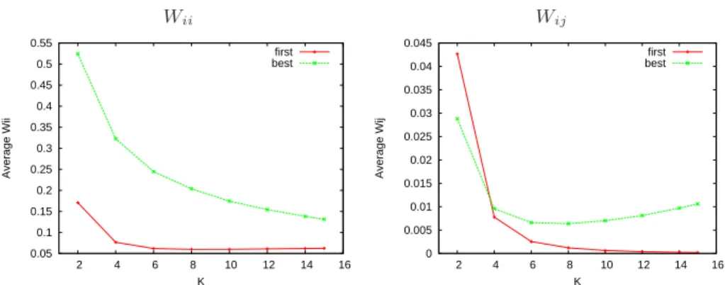
of both the f-LON and b-LON networks on a selected landscape with K = 6, and N = 16. One can see that the weights, i.e. the transition probabilities to neighboring basins are small. The distributions are far from uniform or Poissonian, they are not close to power-laws either. We couldn’t find a simple fit to the curves such as stretched ex-ponentials or exponentially truncated power laws. It can be seen that the distributions differ for the first and best LON models. There is a larger number of edges with low weights for the f-LONs than for the b-LONs. Thus, even though the f-LONs are more densely connected (indeed they are complete graphs) many of the edges have very low weights. Figure 3 (left), shows the averages, over all the nodes in the network, of the weightswii (i.e. the probabilities of remaining in the same basin after a bit-flip
mu-tation) forN = 16 and all the K values. Notice that, for both network models, the weightswiiare much higher when compared to thosewijwithj 6= i (see Fig. 3 right).
Thewiiare much lower for the first than for the best LON. In particular, in the b-LON,
forK = 2, 50% of the random bit-flip mutations will produce a solution within the same basin of attraction, whereas this figure is of less than20% in the f-LON. Indeed, in this case, forK greater than 4, the probabilities of remaining in the same basin fall below10%, which suggests that escaping from local optima would be easier for a first-improvement local searcher.
0 0.01 0.02 0.03 0.04 0.05 0.06 0.07 0.08 0.09 0.1 0.0001 0.001 0.01 0.1 1 P(Wij=w) w first best
Fig. 2. Probability distribution of the network weightswijfor outgoing edges withj 6= i (in logscale on x-axis) forN = 16, K = 6. Averages on 30 independent landscapes.
Wii Wij 0.05 0.1 0.15 0.2 0.25 0.3 0.35 0.4 0.45 0.5 0.55 2 4 6 8 10 12 14 16 Average Wii K first best 0 0.005 0.01 0.015 0.02 0.025 0.03 0.035 0.04 0.045 2 4 6 8 10 12 14 16 Average Wij K first best
Fig. 3. Averages ofwiiweights (left), and averages ofwijwithj 6= i weights (right), for land-scapes withN = 16 and all the K values.
3.2 Basins of attraction features
The previous section studied and compared the basic network features and connectivity of the first and best LONs. The exhaustive extraction of the networks, also produced detailed information of the corresponding basins of attraction. Therefore, this section discusses the most relevant of the basin’s features.
Size of the global optimum basin: When exploring the average size of the global optimum basin of the f-LONs, we found that they decrease exponentially with increas-ing ruggedness (K values). This is consistent with the results for the b-LON on these landscapes [8]. Moreover, the basins sizes for both networks are similar, with those of f-LON being slightly smaller. This may suggest that for the the same number of runs, the success rate of a first-improvement heuristic would be lower. One needs to consider, however, that the number of evaluations per run is smaller in this case.
Basin sizes of the two network models: A comparative study of the basin sizes of the two network models revealed that they are highly correlated. Only the small-est basins of the f-LON model are larger in size when compared to the corresponding smallest basins in the b-LON model.
Basin size and fitness of local optima: Fig. 4 reports the correlation coefficients ρ between the networks’ basin sizes and their fitness, for both the first and best LONs, and landscapes withN = 16 and all the K values. It can be observed that there is a strong correlation between fitness and basin sizes for both types of networks. Indeed, forK ≤ 10, the correlation is over ρ > 0.8. For rugged landscapes, K > 8, the f-LON shows reduced and decreasing coefficients as compared to the b-LON.
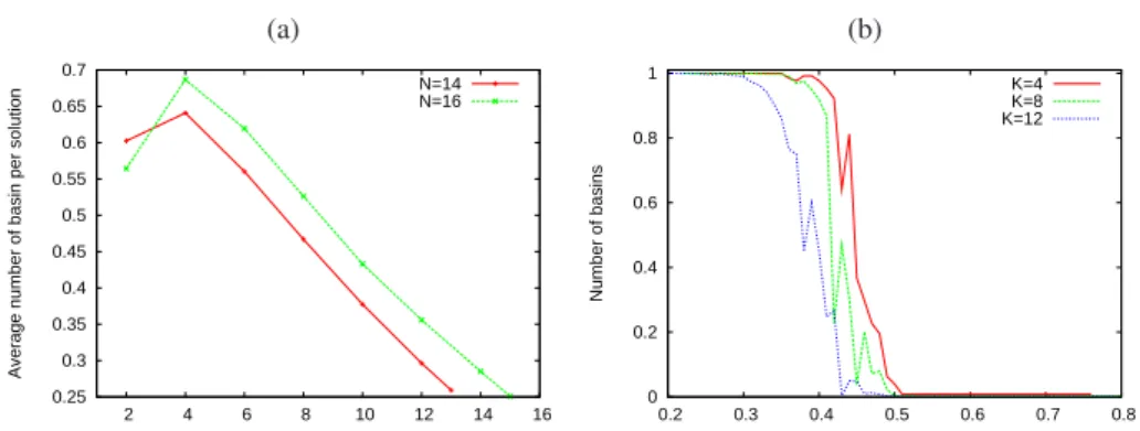
Number of basins per solution on the f-LONs: According to the definition of basins (see section 2), for the f-LON, a given solution may belong to a set of basins. Fig. 5 (a) shows the average number of basins to which a solution belongs (i.e.♯{i | pi(s) >
0}). It can be observed that for N = 16 and K = 4, a solution belongs to nearly 70% of the total number of basins, whereas forK = 14, a solution belongs to less than 30% of the total number of basins. On average, a solution belongs to less basins for highK than for lowK. An exploration of the average number of basin per solution, according to the
0.5 0.55 0.6 0.65 0.7 0.75 0.8 0.85 0.9 2 4 6 8 10 12 14 16 ρ K first best
Fig. 4. Average of the correlation coefficient between the fitness of local optima and their corre-sponding basin sizes on30 independent landscapes for both f-LON and b-LON (N = 16, and all theK values).
solution fitness value (Fig. 5 (b), forN = 16) reveals a striking difference. While low fitness solutions belong to nearly all basins, high fitness solutions belong to at most one basin. The figure suggest the presence of a phase transition, in which the threshold of the transition is lower for highK than for low K. This suggests that the structure of the f-LON network for solutions with high fitness, resembles that of the b-LON, whereas the topology is different with respect to solutions with low fitness.
(a) (b) 0.25 0.3 0.35 0.4 0.45 0.5 0.55 0.6 0.65 0.7 2 4 6 8 10 12 14 16
Average number of basin per solution
K N=14 N=16 0 0.2 0.4 0.6 0.8 1 0.2 0.3 0.4 0.5 0.6 0.7 0.8 Number of basins Fitness K=4 K=8 K=12
Fig. 5. (a) Average number of basins to which a solution belongs. (b) ForN = 16 and 3 selected values ofK, the number of basins per solution according to the solution fitness value. Averages on 30 independent landscapes.
4
Discussion
We have extended the recently proposed Local Optima Network (LON) model to ana-lyze the structural differences between first and best improvement local search, in terms
of the local optima network connectivity and the nature of the corresponding basins of attraction. The results of the analysis, on a set ofN K landscapes can be summarized as follows. The impact of landscape ruggedness (K value) on the network features is similar for both models. First-improvement induces a densely connected network (in-deed a complete network), while this is not the case on the best-improvement model. However, many of the edges in the f-LON networks have very low weights. In par-ticular, the self-connections (i.e. the probabilities of remaining in the same basin after a bit-flip mutation), are much smaller in the f-LON than in the b-LON model, which suggests that escaping from local optima would be easier for a first-improvement lo-cal searcher. The path lengths between lolo-cal optima, and between any optima and the global optimum, are generally larger in f-LON than in b-LON networks. We must con-sider, however, that the number of evaluations needed to explore a basin, would beN times lower for first-improvement than for best-improvement. We, therefore, suggest that first-improvement is a better heuristic for exploringN K landscapes. Our prelimi-nary empirical results support this insight, a detailed account of them will be presented elsewhere due to space restrictions. Most of our work on the local optima model has been based on binary spaces andN K landscapes. However, we have recently started the exploration of permutation search spaces, specifically the Quadratic Assignment Prob-lem (QAP) [2], which opens up the possibility of analyzing other permutation based problems such as the traveling salesman and the permutation flow shop problems. Our current definition of transition probabilities, although very informative, produces highly connected networks, which are not easy to study. Therefore, we are currently consid-ering alternative definitions and threshold values for the connectivity. Finally, although the local optima network model is still under development, we argue that it offers an alternative view of combinatorial fitness landscapes, which can potentially contribute to both our understanding of problem difficulty, and the design of effective heuristic search algorithms.
References
1. M. Barth´elemy, A. Barrat, R. Pastor-Satorras, and A. Vespignani. Characterization and mod-eling of weighted networks. Physica A, 346:34–43, 2005.
2. F. Daolio, S. Verel, G. Ochoa, and M. Tomassini. Local optima networks of the quadratic assignment problem. In Proceedings of the 2010 Congress on Evolutionary Computation, CEC 2010, 2010. (to appear).
3. J. P. K. Doye. The network topology of a potential energy landscape: a static scale-free network. Phys. Rev. Lett., 88:238701, 2002.
4. S. A. Kauffman. The Origins of Order. Oxford University Press, New York, 1993.
5. M. E. J. Newman. The structure and function of complex networks. SIAM Review, 45:167– 256, 2003.
6. G. Ochoa, M. Tomassini, S. Verel, and C. Darabos. A study of NK landscapes’ basins and local optima networks. In Genetic and Evolutionary Computation Conference, GECCO 2008, pages 555–562. ACM, 2008.
7. P. F. Stadler. Fitness landscapes. In M. L¨assig and Valleriani, editors, Biological Evolution and Statistical Physics, volume 585 of Lecture Notes Physics, pages 187–207, Heidelberg, 2002. Springer-Verlag.
8. M. Tomassini, S. Verel, and G. Ochoa. Complex-network analysis of combinatorial spaces: The NK landscape case. Phys. Rev. E, 78(6):066114, 2008.
9. S. Verel, G. Ochoa, and M. Tomassini. Local optima networks of NK landscapes with neu-trality. IEEE Transactions on Evolutionary Computation, 2010. (to appear).