HAL Id: hal-01526090
https://hal.archives-ouvertes.fr/hal-01526090
Submitted on 22 May 2017
HAL is a multi-disciplinary open access
archive for the deposit and dissemination of
sci-entific research documents, whether they are
pub-lished or not. The documents may come from
teaching and research institutions in France or
abroad, or from public or private research centers.
L’archive ouverte pluridisciplinaire HAL, est
destinée au dépôt et à la diffusion de documents
scientifiques de niveau recherche, publiés ou non,
émanant des établissements d’enseignement et de
recherche français ou étrangers, des laboratoires
publics ou privés.
Multi-scale spatial sensitivity analysis of a model for
economic appraisal of flood risk management policies
Nathalie Saint-Geours, Jean-Stéphane Bailly, Frédéric Grelot, Christian
Lavergne
To cite this version:
Nathalie Saint-Geours, Jean-Stéphane Bailly, Frédéric Grelot, Christian Lavergne. Multi-scale spatial
sensitivity analysis of a model for economic appraisal of flood risk management policies. Environmental
Modelling and Software, Elsevier, 2014, 60 (60), pp.153-166. �10.1016/j.envsoft.2014.06.012�.
�hal-01526090�
Multi-scale spatial sensitivity analysis of a model for economic
appraisal of flood risk management policies
Nathalie Saint-Geours
a, *, Jean-Ste
phane Bailly
a, b, Fre
de ric Grelot
c, Christian Lavergne
da
Irstea, UMR TETIS, 500 rue J.F. Breton BP 5095, F-34196 Montpellier, France
b
AgroParisTech, UMR LISAH, 2 place Pierre Viala, F-34060 Montpellier, France
c
Irstea, UMR G-EAU, 361 rue J.F. Breton BP 5095, F-34196 Montpellier, France
d
Universit e Montpellier 3, I3M, Montpellier, France Software availability
Name of software: NOE
Description: The NOE model computes expected annual flood damages at the scale of individual flood-exposed assets, from a given situation, i.e. from a land use map, a set of water depth maps, and a set of depthedamage curves. It also computes expected annual avoided damages at the same scale, when comparing one situation with another. Developers: N. Saint-Geours, T. Langer, F. Grelot and J.-S. Bailly Source language: Python (arcpy library) and R
Software required: ArcGIS© Availability: Contact the developers
1. Introduction
Among the numerical models which are used to investigate environmental issues, many rely on spatially distributed data, such as Digital Terrain Models (DTM), soil maps, land use maps, etc. These spatially distributed models, or simply spatial models, allow for an explicit description of the spatial structures, spatial inter- dependencies, and spatial dynamics involved in the physical, bio- logical, or anthropogenic processes under study. However, it is now well known that all numerical modelsdincluding spatially distrib- uted onesdare fraught with uncertainties, which may stem from a lack of knowledge about the phenomena under study, from the natural variability of the quantities of interest, from measurement errors, model assumptions, or numerical approximations (Walker et al., 2003). Hence, when a spatial model is used as a support tool for decision-making, one must remember that “anyone using un- certain informationdmeaning the overwhelming majority of mapped data usersdshould consider carefully the possible sources of uncer- tainty and how to deal with them” (Fisher et al., 2005).
To address this issue, a number of uncertainty analysis (UA) and sensitivity analysis (SA) methods, both qualitative and quantitative,
have been developed over the last decade (Saltelli et al., 2008). They study how model outputs react when input variables are uncertain. UA focuses on the propagation of uncertainties throughout the model and aims to quantify the resulting variability of the model output. SA seeks to study how the uncertainty in a model output can be apportioned to the uncertainties in each of the model inputs. It allows input variables to be ranked according to their contribu- tion to the output variability. SA thus helps to identify the key input variables, those that determine the final decision of the model end- user, and on which further research should be carried out. UA and SA methods have been gradually adopted by modellers in different disciplinary fields, especially in environmental research (Ascough et al., 2008; Cariboni et al., 2007; Tarantola et al., 2002), and today are widely recognized as essential steps in model building (CREM, 2009; European Commission, 2009). One of the most common SA approach is variance-based global sensitivity analysis (VB-GSA), which widely explores the space of input uncertainties (global method), and does not require any preliminary hypothesis (linearity, regularity) regarding the model under study (Saltelli et al., 2008).
However, partly because of the curse of dimensionality, SA methods have seldom been applied to environmental models with both spatially distributed inputs and outputs. A few recent works have tried to tackle this issue (Lilburne and Tarantola, 2009, for a review). Both Ruffo et al. (2006) and Saint-Geours et al. (2013) used geostatistics to simulate the uncertainty on spatially distributed model inputs and incorporate them into a VB-GSA approach. Moreau et al. (2013) investigated the sensitivity of the agro- hydrological TNT2 model to five different soil-map patterns, mak- ing use of a fractional factorial design to carry out an analysis of variance, while Chen et al. (2013) recently discussed sensitivity analysis for spatial multi-criteria decision making models. In addition, other authors developed new procedures to compute sensitivity indices for a spatial model output, either with respect to its spatial average (Lilburne and Tarantola, 2009) or with respect to the values of the model output at each point of a study area (Heuvelink et al., 2010; Marrel et al., 2011). A number of recent papers also deal with the issue of CPU time expensive environ- mental models, for which standard sensitivity analysis techniques cannot be applied; in this case, the construction of a cheap meta- model (emulator) is often necessary, see (Petropoulos et al., 2013) for a recent illustration on the SimSphere soilevegetationeatmo- sphere-transfer model. The design of such meta-models for expensive computer codes with spatially distributed inputs and outputs is still an open research question (Marrel et al., 2011).
Nevertheless, to date, none of these studies has reported on a key question: the link between UA/SA and spatial scale issues. Indeed, in many environmental models, the end users are inter- ested in the aggregated value of some spatially distributed model output over a given spatial unit v. In most cases, the aggregated value is just the linear average or the sum of model output over v (e.g., the average porosity of a block, the total evapotranspiration over a plot of land, etc.). But Heuvelink (1998) observed that under a change of spatial support v, the relative contribution of uncertain model inputs to the variability of the aggregated model output may change. Hence, in a spatial model, the results of UA/SA depend on the spatial scale of the problem. Unfortunately, the notion of spatial scaledmade up of the scale triplet (Blo€schl and Sivapalan, 1995): spatial extent, support, spacingdis mostly ignored in the mathe- matical frameworks of SA methods. Among scale issues, the so- called change of support problem has long been discussed in the field of geostatistics: we know that the variance of an uncertain spatially distributed quantity depends on the spatial support v over which it is aggregated. Up to our knowledge, only Saint-Geours et al. (2012) tried to translate this problem into the context of
variance-based GSA. On a simple model, they showed how the sensitivity indices of model inputs depend on the spatial support v over which the model output is aggregated; denoting with p(v) the ratio of sensitivity indices of spatially distributed model inputs vs non-spatial inputs, they found a relation of the form p(v) ¼ vc/jvj, with jvj the surface area of v and vc some critical value. When the model output is aggregated on a spatial support of area jvj smaller than vc, the ratio p(v) is larger than 1, which means that the sensitivity indices of spatially distributed inputs are larger than those of non-spatial inputs, and thus that spatially distributed in- puts contribute more to the variance of model output than non- spatial inputs. On the contrary, if jvj is larger than vc, then
p(v) 1, and the non-spatial inputs are key contributors to model output variability. However, their work was mainly theoretical, and their results only valid under restrictive assumptions of inputs stationarity and model additivity. In particular, they did not examine if their conclusions would hold on a real, complex test case.
The aim of this paper is thus to investigate, on an applied case study, how the results of an uncertainty and sensitivity analysis interact with a change of spatial support of the model output. We discuss this question through a complete case study on a model for economic assessment of flood risk management policies, named NOE (Saint-Geours et al., 2013). The NOE model has both spatially distributed inputs (topography, map of water heights, land use map, etc.), and spatially distributed outputs (avoided flood damage indicators). A number of recent studies already performed UA/SA of flood damage assessment models, in whole or in parts (Apel et al., 2008). Most of these studies are limited to the forward propagation of uncertainty (UA), the perimeter of which can vary from a single module of the complete modelde.g., land use (Te Linde et al., 2011), hydraulic simulation (Bales and Wagner, 2009), estimation of damages (Koivuma€ki et al., 2010)dup to the entire modelling chain (de Kort and Booij, 2007; Qi and Altinakar, 2011). Fewer publica- tions address the issue of ranking the various sources of uncertainty with SA (de Moel et al., 2012). In particular, Saint-Geours et al. (2013) already carried out VB-GSA on the NOE model over the Orb Delta, France. However, in this study, they disregarded spatial scale issues: sensitivity indices were only computed with respect to the aggregated value of model output over the entire floodplain, without examining model behaviour at finer spatial scales. There are at least two motivations for an in-depth study of this issue. First, it would bring a better understanding of the behaviour of the NOE model, by identifying the key input variables at different spatial scales. Next, analysing the uncertainty and sensitivity of NOE model outputs at different spatial scales would provide the model end- users (i.e., local water managers) with a more complete informa- tion and may help them in their decision making.
In order to demonstrate how UA/SA can bring a new insight into scaling issues in spatial modelling, we perform a multi-scale VB-GSA of the NOE model. Our idea is to compute variance-based sensi- tivity indices with respect to the NOE outputs aggregated over different spatial supports v. We will try to answer the following questions: what is the uncertainty of the NOE output, at different spatial scales? What are the key input variables that explain the largest fraction of the variance of the NOE output, at different spatial scales? How does the uncertainty of the NOE output, and the related sensitivity indices, vary in space, at a fixed spatial scale?
The next section (Section 2) starts with some relevant back- ground information on the selected study site (the Orb Delta), and presents the NOE model. Next, we display a brief introduction to the concepts of VB-GSA, and portray into details how we simulated the uncertainty sources in the NOE model, propagated them with Monte-Carlo simulations, and how we computed multi-scale vari- ance-based sensitivity indices (Section 3). The results consist of
Fig. 1. The study site is located in He rault de partement, south of France. The Orb River flows southward. Flood risk management plan includes various structural flood mitigation measures.
both uncertainty maps and sensitivity maps that allow us to identify the key input variables in the NOE model at different spatial scales (Section 4). We discuss the main outcomes and limits of our study in Section 5.
2. The NOE model, study site and data
The NOE model and its implementation on the Orb Delta, France, were already fully described by Saint-Geours et al. (2013). In this section, we only reproduce the key points that are necessary to the understanding of our present work.
Flood hazard modelling
Flood exposure modelling
Damage estimation
Expected Annual Avoided Damage
Fig. 2. Simplified flowchart of the NOE model. 2.1. Study site: the Orb Delta hydraulic, GIS and economic modules.
1The main model output is
The Orb Delta is a catchment of 63 sq. km located in the south of France, surrounding a 15 km reach of the Lower Orb River from Be ziers city to the Mediterranean sea (Fig. 1). It has a typical Medi- terranean subhumid regime, with an annual maximum discharge ranging from 100 to 1800 m3/s from year to year at the main gauging station on the Delta (Tabarka gauge, Fig. 1). The Orb Delta includes the cities of Be ziers, Portiragnes, Sauvian, Se rignan, Valras-Plage and Villeneuve-le s-Be ziers. It is covered for one third by cultivated land. About 16,000 people live permanently in the flood prone area, which also hosts 774 companies and 30 seaside campgrounds, gathering up to 100,000 tourists in summertime. In December 1995, a flooding event with a peak discharge of 1700 m3/s at Tabarka gauge caused around 53 MV in material losses (Erdlenbruch et al., 2008). In 2001, local authorities reacted and launched a flood risk management project, mainly based on various structural mitigation measures, including dyke strengthening around urban areas, restoration of sea outfalls and channel hydraulic improvement (SMVOL, 2011). Avail- able data on the area include aerial photographs, a 5 m-cell-size DTM built from photogrammetry, the annual maximum flow series from 1967 to 2009 at the Tabarka gauge (referred to as the AMFS dataset), and various spatial datasets on buildings, cultivated land and eco- nomic activities.
2.2. The NOE model
The NOE model is used to estimate the flood damage reduction which will result from the implementation of flood mitigation measures on the Orb Delta. It is a combination of hydrological,
the Expected Annual Avoided Damage (DEAD [V/year]) over the floodplain, that is, the amount of annual expected flood losses that will be reduced thanks to the flood mitigation measures. We briefly present here the main processes of the NOE model (Fig. 2). 2.2.1. Flood hazard modelling
The DEAD indicator is computed from a range of six potential flood events of various magnitudes, denoted by e1ee6, with increasing maximum discharges q1eq6 (Table 1). These flood events include both historical floods (e3, e4), and floods which were simu- lated with a rainfallerunoff model (e1, e2, e5, e6). Their annual ex- ceedance frequencies f1ef6 were computed from the AMFS dataset, which was fitted by a Gumbel dischargeefrequency curve. Next, for each flood event ei, i ¼ 1,…,6, the water flow over the floodplain was simulated using Isis Flow, a 1D step-backwater hydraulic model (ISIS, 2012). These flow simulations were then combined with the DTM, to produce maps of maximum water depths over the Orb Delta. These computations were carried out both before and after the enforcement of flood mitigation measures.
2.2.2. Flood exposure modelling
To carry out flood exposure analysis, a detailed land use geo- databasedreferred to as the assets mapdof the entire Orb Delta was built from various data sources (Fig. 3). Four types of flood-
1
It must be emphasized that the NOE model is just one possible implementation of a wider, more generic framework for flood damage assessment, that has been used by many authors on various floodplains around Europe (Merz et al., 2010).
Table 1
Main characteristics of flood events e1 to e6: maximum discharge q at Tabarka gauge,
annual exceedance frequency f, and corresponding return interval T ¼ 1/f. Flood event description q [m3/s] f T [years]
e1 Smallest eventa 1018 0.2 5
e2 10-Year design flood 1287 0.1 10
e3 Historical flood (Dec. 1987) 1696 0.0333 30
e4 Historical flood (Jan. 1996) 1882 0.02 50
e5 Large design flood 2133 0.01 100
e6 Extreme floodb 3000 0.001 1000
a Event e1 is supposed to be the smallest flood event for which damages occur. b Event e 6 would result in an over-topping of all existing flood-control dykes. exposed assets are considered: private housing units (individual buildings), plots of cultivated land, campgrounds, and other eco- nomic activities. The assets map describes each asset by an indi- Table 2 Content of the assets map. Type of assets # objects Total surface [sq. km] Private housing 16,436 1.37 Cultivated land 707 23.36 Campgrounds 111 1.02 Other economic activities 691 0.62 2.2.4. Computation of the expected annual avoided damage The expected annual damage (EAD [V/year]) is a common in- dicator used to measure potential flood damages over a given floodplain (Arnell, 1989). It can be defined as the mathematical expectation of flood damages D(e) over the space of possible flood events e. Using the annual exceedance frequencies f of flood events, vidual polygonal object in a GIS vector layer at the 1:5000 scale (Table 2), and each object is further characterized by its subtype, its we have: EAD ¼ Z 1 Dðf Þdf (resp. EAD0 ¼ 0 Z 1 D0 ðf Þdf ). This integral 0 ground floor elevation, its floor surface area, etc. Flood exposure is assessed by overlaying the assets map with water depth maps, and by computing the average water depth over each individual polygonal object. 2.2.3. Damage estimation In this study, flood damage assessment only includes direct and tangible monetary lossesdMerz et al. (2010) list the other types of flood-induced damages that should be considered for a more complete analysis. For each flood event e1ee6, the total damage cost before (resp. after) the enforcement of flood mitigation measures is denoted by Di (resp. D0 ), and DD i ¼ Di D0 denotes the damage can be approximated with a simple trapezoidal ruledamong other integration methodsdfrom the range of flood events e1ee6 with annual exceedance frequencies f1ef6 and corresponding damages D1eD6 (resp. D0 to D0 ). In the present study, the main output of 1 6
interest is the reduction of potential flood damages that will result from the enforcement of flood mitigation measures on the Orb Delta, i.e., the variation: DEAD ¼ EAD EAD0 (1)
One key point is that the DEAD indicator [V/year] can be dis- played at different spatial scales. It is first computed for each indi-i indi-i vindi-idual asset over the floodplaindi-in, and mapped, but indi-it can also be reduction brought by the mitigation measures. Damage estimates
are computed for each flood-exposed asset from flood exposure data, using a set of 94 depthedamage curves, one for each combi- nation of type, subtype of assets and season of flood occurrence (SMVOL, 2011). These depthedamage curves link the average water depth over the asset with a value of damage per unit area of floor surface [V/sq.m.]dfor cultivated land, private housing, and camp- groundsdor with a total value of damage [V]dfor other economic activities. As a coarse approximation, flood velocity and flood duration were considered to be homogeneous over the entire study area.
summed up over any spatial unit v (e.g., an administrative district within the floodplain), or even aggregated over the entire Orb Delta. 3. Methods
3.1. Overview
Multi-scale VB-GSA of the NOE model aims to assess the un- certainty of the DEAD indicator, to compute the associated variance-based sensitivity indices, and to investigate: i) how these uncertainty and sensitivity measures depend on the spatial support
2 Propagating uncertainty (Monte-Carlo simulation) 1 Table 3
Sources of uncertainty in the NOE model. A set of nj random realisations is sampled
for each uncertain input Xj.
Model input nja Model of uncertainty
Modelling uncertainty on model inputs
- flood frequencies - water depth maps - assets map - depth-damage curves NOE model Inputs Outputs 3 Estimating variance-based sensitivity indices Resulting uncertainty on model outputs - ΔEAD maps - aggregated ΔEAD over different spatial units X1 Exceedance frequencies X2 Water depth maps 1000 Confidence interval on the fitted Gumbel dischargeefrequency curve.
100 Errors in hydraulic modelling are not taken into account; Measurement errors in DTM are modelled by a Gaussian noise with spatial auto-correlation. Fig. 4. Flowchart for multi-scale VB-GSA of the NOE model.
of the DEAD indicator; and ii) how they vary in space, for a fixed output scale. In the first step of the analysis (Fig. 4), sources of uncertainty in the NOE model are identified and described in a probabilistic framework, and a set of random realisations is sampled for each uncertain model input (Section 3.2). Next, pseudo-Monte Carlo simulations are used to explore the space of
X3 Assets map 1000 Misclassification of
land use types: confusion matrix;
Variability of ground floor elevation of assets: empirical pdf from field survey; Surface area of polygonal objects: random multiplying coefficient drawn from uniform pdf.
input uncertainty and propagate uncertainty through the NOE model (Section 3.3). Variance-based sensitivity indices are then computed to rank the uncertain model inputs, depending on their contribution to the variance of the DEAD indicator (Section 3.4).
X4 Depthedamage
curves
1000 For each depthedamage curve, random multiplying coefficient εk drawn from
uniform pdf U ½0:5; 1:5 ; εk
are independent. These steps were already presented in a single-scale VB-GSA of the
NOE model (Saint-Geours et al., 2013), thus we only reproduce here the key elements that are necessary to the understanding of the present work. We then go one step further, by computing sensitivity indices in a multi-scale framework (Section 3.5): sensitivity indices are computed with respect to the aggregated value of the DEAD output indicator over cells of different sizes. For each cell size, we compute both uncertainty maps and sensitivity maps, that allow us to discuss the relation between VB-GSA and spatial scale issues. 3.2. Modelling sources of uncertainty
The first step of the analysis is to list the uncertainty sources in the NOE model, then to describe and simulate them in a probabi- listic setting, using residual analysis, external data or expert opinion. Four uncertain inputs are considered (Table 3): the flood annual exceedance frequencies (X1), the assets map (X2), the water depth maps (X3), and the depthedamage curves (X4). A set of nj ¼ 100e1000 random realisations is sampled for each of them. 3.2.1. Uncertainty in flood annual exceedance frequencies (X1)
Uncertainty in the computation of flood annual exceedance frequencies fi may arise from stream gauge measurement errors, non-stationarity of hydrologic series due to climate change, but also from the choice of an extreme value distribution to fit a dis- chargeefrequency relationship to the AMFS dataset, and from the statistical uncertainty of this fit. Here, only the latter uncertainty was taken into account, which we acknowledge is only a small part of the overall uncertainty in fi. Empirical confidence bounds (Fig. 5) were computed around the nominal Gumbel curve fitted on the AMFS dataset (Maidment, 1993), and a set of n1 ¼ 103 Gumbel curves were then randomly sampled from the joint distribution of the fitted parameters. From this set of curves, n1 ¼ 103 exceedance frequencies fi, and associated return intervals Ti ¼ 1/fi, were generated for each flood event ei, i ¼ 1,…,6 (Fig. 6), with an addi- tional white noise following normal distribution N ð0; s2 Þ with s2 the empirical standard deviation of residuals.
a
One can note that the number nj of random realisations is not the same for each
model input: these numbers were chosen under constraints of CPU time and storage space.
3.2.2. Uncertainty in water depth maps (X2)
An in-depth investigation of the uncertainties arising in hy- draulic modelling goes well beyond the scope of the present study. Following Bales and Wagner (2009) and Koivuma€ki et al. (2010), who suggest that high-resolution topographic data is the most important input for accurate inundation maps, we focused on one single source of uncertainty in the water depth maps: the mea- surement and interpolation errors in the 5 m-cell-size DTM. These errors are spatially auto-correlated and are modelled by a Gaussian 2D random field with an exponential variogram model, whose parameters were determined from a set of 500 control field points (sill 17 cm, range 500 m, nugget 0.02). A set of n2 ¼ 100 random realisations of the random error field is then generated using SGeMS software (Remy et al., 2009), and added as noise to the nominal water depth maps.
3.2.3. Uncertainty in the assets map (X3)
Three uncertainty sources in the assets map are considered: misclassification of polygonal objects, measurement errors in the surface area of assets, and variability of the ground floor elevation of assets. We first built a confusion matrix (Fisher, 1991), based on expert opinion, to account for possible misclassifications in the assets map (Table 4). Next, due to digitalising errorsdabout 0.3 mm at the map scale (Hengl, 2006), the surface area of polygonal objects in the assets map is uncertain; we thus multiplied the nominal surface of each asset by a corrective random coefficient in ±6% (uniform pdf). Third, the empirical pdf of ground floor elevation of assets was estimated from a field survey (100 sampled assets, de- tails given in Saint-Geours et al. (2013, Fig. 7)). A total number of n3 ¼ 1000 randomized assets map was sampled, combining these three sources of uncertainty.
Table 4
Confusion matrix of the assets map.
Fig. 5. AMFS dataset from 1967 to 2009 and fitted Gumbel distribution (solid line) with 95% confidence bounds (dashed lines).
Land use type Number of sub-types
Probability of confusion between sub-types Private housing 1 No confusion. Cultivated land 15 25% chance of confusion
between durum wheat and bread wheat; 10% chance of confusion between colza, maize, barley and sunflower; 25% chance of confusion between permanent and temporary grassland. Campgrounds 18 No confusion.
Other economic 60 0.17% chance of belonging activities to each other class of economic
activities.
3.3. Propagating uncertainty through the NOE model
Once each model input has been sampled, uncertainty is propagated through the NOE model using Monte Carlo simulation. Numerous pseudo-Monte Carlo sampling schemes have been suggested in the UA/SA literature to efficiently estimate the share of output variance that is explained by each uncertain model input. In this study, we choose to use the Sobol' sampling scheme (Sobol', 1993), also referred to as the pick and freeze scheme, based on the use of LP-t quasi-random sequences which are known to increase the convergence rate of estimates of high-dimensional integrals (Sobol', 1967). Total sample size is equal to N ¼ n $ (p þ 2) ¼ 24,576 where p ¼ 4 is the number of inputs and n ¼ 4096 is the base size of LP-t quasi-random sequences; it is chosen to be large enough to obtain a satisfactory level of accuracy for the sensitivity indices estimates. The four uncertain model inputs X1eX4 are assumed to be mutually uncorrelated. The ith line of the quasi Monte Carlo sample is an input set ðXðiÞ ðiÞ ðiÞ ðiÞ ðiÞ
Fig. 6. Empirical distributions of return intervals Ti for flood events e1ee6. Sample size
n1 ¼ 1000.
3.2.4. Uncertainty in depthedamage curves (X4)
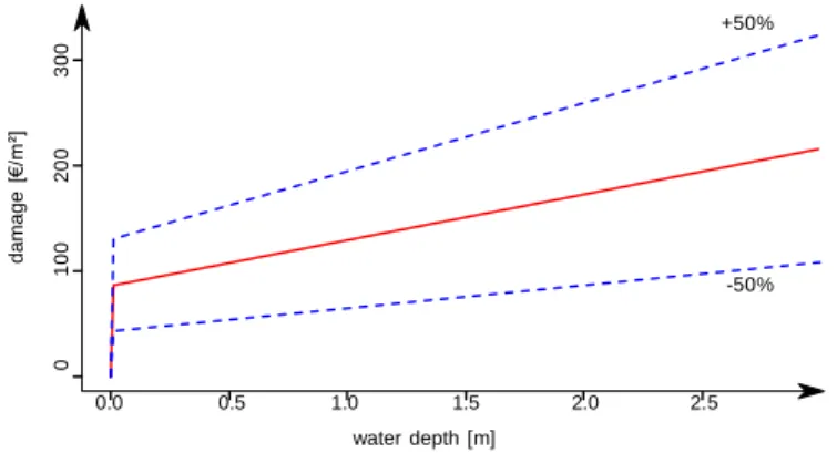
Uncertainty in depthedamage curves has been extensively discussed in previous flood damage assessment studies (Koivumaki et al., 2010; Merz et al., 2010; de Moel and Aerts, 2011). Here, we represent the uncertainty on the set of 94 depthedamage curves by a uniform pdf, defining a 50% to þ50% range around nominal curves (Fig. 7).2 Random depthedamage curves associated with each land use type and subtype are sampled independently3 (sample size n4 ¼ 1000).
2
The [ 50%, þ50%] uncertainty range is chosen based on expert opinion. It is in line with Torterotot (1993) who studied the uncertainty on depthedamage curves for private housing and displayed coefficients of variation around 40%. Other au- thors could choose a much larger range (Merz et al., 2010).
3
Note that this model of uncertainty is different from that of de Moel and Aerts (2011), who sampled randomized depthedamage curves collectively for all types of assets, from a single p-value. Saint-Geours (2012, p.172) explains how the hy- pothesis of independence or homogeneity of the depthedamage curves over different types of assets will induce more or less cancelling-out effects at aggre- gated scales.
1 ; X2 ; X3 ; X4 Þ where Xj is sampled with replacement from the set of nj pre-generated random realisations of the jth model input. Note that with such large value of n, the same realizations of a given input Xi can be sampled several times during the experi- ment. The NOE model is then run for the N input sets, for a total CPU time of 24 h on a 6-nodes cluster computer.
3.4. Variance-based sensitivity indices
Variance-based total-order4 sensitivity indices of each uncertain model input with respect to any output of interest can be estimated from the set of N model runs, using ad hoc estimators given by Lilburne and Tarantola (2009). These sensitivity indices measure the contribution of a given model input (and its interactions with other inputs) to the variance of a given model output. More pre- cisely, let us consider some model Y ¼ f(X1,…,Xp) with p model inputs. Model inputs Xj are treated as independent random vari- ables; hence the model output Y is also a random variable. The variance-based total-order sensitivity index of Xj, denoted by STj, measures the share of total output variance var(Y) that is explained
4
In this study, we computed both first-order and total-order sensitivity indices, but we deliberately chose to display only total-order indices for the following reasons: i) preliminary results showed that first-order and total-order indices were close, indicating that interactions between model inputs do not contribute much to model output variance, ii) empirical confidence bounds of total-order indices, computed by bootstrap using 100 replicas, proved to be narrower than that of first- order indices, and iii) first-order and total-order indices displayed the same behaviour with respect to change of spatial support, which is the focus of our study.
j j j j d a m a g e [€ /m ²] 0 100 200 300 ¼
+50% with respect to the sum of the DEAD indicator over ck, from the set of N model runs;
2. the set of sensitivity indices fSTa j kðc Þg over all the cells ck builds a grid map that we denote by
size a for the jth model input.
STa and call sensitivity map of cell
Following this procedure, we obtain 4 4 ¼ 16 sensitivity maps STa j j. Next, in order to compare the sensitivity maps STa obtained for -50% various cell sizes a, we summarize each sensitivity map by a single
scalar measure. For each cell size a ¼ 0.04, 0.16, 0.64, and 2.56 sq. km., and for the jth model input, we calculate the average value of the sensitivity map STa , and denote it by STa :
0.0 0.5 1.0 1.5 2.0 2.5 water depth [m]
j j 1 Ga
Fig. 7. Nominal depthedamage curve for private housing (solid line) with a [ 50%; þ50%] uncertainty range (dashed lines).
STa Ga
X
STa ðck Þ (3) k¼1
by model input Xj and by the interactions of Xj with the other model inputs. It is defined as
h i
in which Ga denotes the total n umber of cells ck in the grid map of cell size a. This average index STa is scale-dependent: it measures the average contribution of the jth model input to the variance of the DEAD indicator aggregated over small cells of area a.
E var Y X j Finally, to complete the analysis, we also compute sensitivity STj ¼
e
varðY Þ (2) indices STj of model inputs X1eX4 with respect to the aggregated value of the DEAD indicator over the entire floodplain (surface area in which X j
Sensitivity e ¼ ðX
k Þksj denotes the set of all model inputs but Xj. x ST 2 [0;1] is the expected residual part of output
a ¼ 63 sq. km.). inde j
variance if all model inputs but Xj were fixed. The sum of total-order sensitivity indices is always more than 1. Total-order sensitivity indices STj can be used to identify the model inputs that account for most of the model output variability, and they may lead to model simplification by identifying model inputs that have little influence on the model output variance. Please refer to Saltelli et al. (2008) or Plischke (2012) for more details on the definition and estimation of variance-based sensitivity indices.
3.5. Multi-scale VB-GSA
To investigate scale issues in the NOE model, we carry out a multi-scale analysis by computing sensitivity indices STj with respect to the aggregated value of the DEAD indicator over different spatial supports of increasing area.
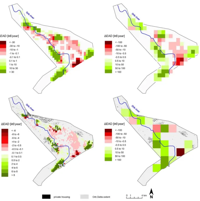
First, for each of the N ¼ 24,576 simulations, the NOE output datadi.e., the DEAD indicator computed for each individual asset over the floodplaindis transformed into a number of grid maps of increasing cell sizes: a DEAD grid map is obtained by computing at each cell ck of the grid the sum of the DEAD indicator over all assets (or parts of assets) contained in the cell.5 We consider four different grid maps with cells of 200 m by 200 m, 400 m by 400 m, 800 m by 800 m and 1600 m by 1600 m, and corresponding cell sizes
a ¼ 0.04, 0.16, 0.64 and 2.56 sq. km, respectively. Fig. 8 shows the
DEAD grid maps produced using the nominal values of the NOE model inputs.
Then, grid maps of sensitivity indices are produced by computing total-order sensitivity indices STj with respect to the aggregated value of the DEAD indicator at each cell of the various
DEAD grid maps. More precisely, for each cell size a ¼ 0.04, 0.16, 0.64, and 2.56 sq. km, and for each model input Xj, j ¼ 1,…,4, we proceed as follows:
4. Results
4.1. Uncertainty analysis
Fig. 9 shows a spatially explicit representation of the uncertainty on the DEAD grid map over the N ¼ 24,576 model runsdcell size
a ¼ 0.04 sq. km is taken as an example. A first map displaying the maximum values of DEAD for each cell ck over all model runs (Fig. 9a) is compared to the map of minimum values (Fig. 9b). It appears that for a large number of cells, the minimum and maximum values of DEAD have opposite signs, which we interpret to mean that, due to the uncertainties in the NOE input data, it is impossible to assess with certainty whether these areas will benefit or suffer from the implementation of the flood mitigation measures on the Orb Delta.
By comparing these uncertainty maps with that of land use on the study site (Fig. 3), it can be noted that the cells with uncertain sign are mostly covered with cultivated land and show relatively small values of positive or negative DEAD. On the contrary, for cells ck that include urban areas, campgrounds and other economic ac- tivities, the DEAD indicator proves to keep a constant sign over all model runs, with larger positive or negative values. Hence, in spite of the numerous uncertainties that were considered in the analysis, we can conclude that the flood risk management plan will almost certainly result in a reduction of the expected annual damages on urban areas, and almost certainly result in an increase of damages on campgrounds. In addition, cells ck that include urban areas or campgrounds show large standard deviations and low coefficients of variation of the DEAD indicator (Fig. 9c and d), while cells only covered with cultivated land have small standard deviations but larger coefficients of variation.
Table 5 summarises the outcomes of the uncertainty analysis for floodplain: it gives the 1. at each cell ck of the DEAD grid map of cell size a, we compute
the total-order sensitivity index STa ðc Þ of the jth model input
each cell size a, as well as for the entire
average value (over the cells ck of size a) of the mean, standard j k
deviation and coefficient of variation of the DEAD indicator over N ¼ 24,576 model runs. The mean value and standard deviation of
5
If an asset has a large surface area and overlaps many cells of the grid, then the value of the DEAD indicator over this asset is shared out among the cells in pro- portion to the overlaped areas.
the DEAD indicator naturally increase with the surface area a of the cells over which it is aggregated, ranging from 3.731 ± 1.380 kV/ year for smallest cell size to 5459 ± 1110 kV/year for the entire
j
j
Fig. 8. DEAD grid maps for nominal values of the model inputs, cell size a ¼ 0.04 sq. km (bottom left), a ¼ 0.16 sq. km (top left), a ¼ 0.64 sq. km (top right) and a ¼ 2.56 sq. km (bottom right).
floodplain. However, if we consider a dimensionless measure of variability such as the coefficient of variation, we observe a different behaviour: the coefficient of variation of the DEAD indi- cator decreases with the surface area of the cells. This finding corroborates the idea that some spatial averaging-out effects result in a reduction of the relative uncertainty when the DEAD indicator is aggregated over a large spatial unit.
4.2. Sensitivity analysis
Fig. 10 displays the sensitivity maps STa for each model input and for both the smallest and largest cell size a. Spatial distribution of sensitivity indices proves to be heterogeneous. By comparing the first sensitivity maps (a ¼ 0.04 sq. km) with the map of land use on the study site (Fig. 3), we can identify two different types of areas: urban areas and cultivated land. On the cells that include urban areas, the assets map and the hazard maps display smaller sensi- tivity indices than on the cells covered with cultivated land.
Correspondingly, depthedamage curves and flood exceedance frequencies have larger sensitivity indices in urban areas than on cultivated land. This finding might be explained by comparing the characteristics of depthedamage curves for private housing assets and agricultural assets. In particular, depthedamage curves for cultivated land are simple step functions with a number of threshold water levels: when water levels are uncertain, they may induce a jump below or above these thresholds. These jumps might explain that the water depth maps have a larger contribution to the variance of the DEAD indicator for cultivated land than for urban areas.
In addition, we can investigate how a change of spatial support modifies the sensitivity indices in the NOE model, by comparing the sensitivity maps STa for cell sizes a ¼ 0.04 sq. km and a ¼ 2.56 sq. km (Fig. 10 top and bottom, respectively). This comparison clearly sug- gests that the ranking of uncertainty sources depends on the surface area of the cells. The sensitivity indices of the spatially distributed inputs (i.e., the water depth maps and the assets map) decrease from
j
Fig. 9. Uncertainty on the DEAD grid map of cell size a ¼ 0.04 sq. km over N ¼ 24,576 model runs: maximum values (a), minimum values (b), standard deviations (c), and co- efficients of variation (d) at each cell ck. Dashed cells indicate that the sign of DEAD over the cell changes for more than 20% of model runs.
a ¼ 0.04 to a ¼ 2.56 sq. km, while the sensitivity maps of the depthedamage curves and of the flood exceedance frequencies display larger values for cell size a ¼ 2.56 sq. km than for a ¼ 0.04 sq. km. These results offer empirical evidence of the change of support effect on variance-based sensitivity indices, which was described from a theoretical perspective by Saint-Geours et al. (2012): the sensitivity indices of spatially distributed inputs decrease with the size of the spatial support of model output while the sensitivity indices of non-spatially distributed inputs increase.
To better highlight this change of support effect, Fig. 11 displays the average sensitivity indices STa [Eq. (3)] for each model input Xj
and each cell size a, as well as the sensitivity indices STj for the entire floodplain. From these average indices, one can derive a ranking of model inputs at each cell size: for example, the assets map is ranked 1st for cell sizes a ¼ 0.05 to 2.56 sq. km., while it is only ranked 3rd for cell size a ¼ 63 sq. km. The average sensitivity indices of spatially distributed inputs (i.e., the water depth maps and the assets map) prove to decrease with an increase of the area a
over which the model output DEAD is aggregated, while the sensitivity indices of non spatially distributed inputs (depthe- damage curves and flood exceedance frequencies) increase con- trastingly. For a cell size a 2 [5,50] sq. km., both spatially and
non-j
ac
j
Table 5 Correspondingly, when a > ac, non-spatial inputs contribute the
a
Descriptive statistics over N ¼ 24,576 simulations: average values of mean, standard deviation (s.d.) and coefficient of variation (c.var.) of DEAD over all cells ck. Last line
gives descriptive statistics for the sum of DEAD over the entire floodplain (one single cell).
most to model output variance. To test this theoretical relation on the NOE model real case study, we computed for each cell size a
the ratio p(a) of the mean value of average sensitivity indices
STa of
Cell size a [sq. km]
Number of cellsa
Av. mean [kV/yr] Av. s.d. [kV/yr] Av. c.var. [%]
j 0.04 1463 3.7 100 1.4 100 385
and depthedamage curves X4): 0.16 416 1.3 101 4.1 100 247 0.64 128 4.3 101 1.2 101 96 2.56 43 1.3 102 3.2 101 51 STa þ STa 3 3 pðaÞ ¼ 2 3 (5) 63.00 e 5.5 10 1.1 10 20 STa þ STa a
The cells ck for which the mean value of the DEAD indicator over N model runs is nulldi.e., some cells on the edge of the study areadwere not considered to compute these average values.
Fig. 12 shows that p(a) decreases with a, in accordance with Eq. (4). A least squares regression (R2 ¼ 0.79) on log-transformed data points yields an estimate of the critical cell size b ¼ 6:72 sq. km. spatially distributed inputs contribute almost equally to the vari-
ance of the DEAD indicator.
In a previous work, Saint-Geours et al. (2012) used a geo- statistical framework to provedunder restrictive assumptions of inputs stationarity and model additivityda general relation of the form:
pðaÞ ¼ ac =a (4) where p(a) is the ratio of sensitivity indices of spatially distributed model inputs vs non spatial inputs, a the area of the spatial unit over which the model output is aggregated, and ac a so-called critical size which depends both on the model characteristics and on the pdf of uncertain model inputs. This critical size divides the range of a into two zones: if a < ac, then p(a) > 1, which means that sensitivity indices of spatially distributed inputs are larger than those of non-spatial inputs, and thus that spatially distributed in- puts are key contributors to model output variability.
5. Discussion
5.1. Sensitivity analysis and spatial averaging-out effects
Our first goal was to identify the main sources of uncertainty in the NOE model, at different spatial scales. We completed this goal by performing multi-scale VB-GSA on the Orb Delta case study. Our results indicate that for large spatial supports (e.g., the entire floodplain), the main source of uncertainty is the uncertain annual exceedance frequencies of flood events, which explain almost a third of the variance of the DEAD indicator at the floodplain scale. This observation corroborates the conclusions of Apel et al. (2004), who stated that reliable extreme value statistics are crucially important in flood risk modelling. Unfortunately, reducing this input uncertainty is impossible, as it would require longer time series of maximum discharges at gauging stations, which are not available. Besides, we also found that for much smaller spatial
ac
j
b ¼ 6:72 sq.
j
study (Fig. 12), even if the restrictive assumptions discussed in (Saint-Geours et al., 2012) are not fulfilleddin particular, NOE un- certain spatial inputs such as water depth maps or the assets map are not stationary random fields. Based on Eq. (4), we could esti-mate the critical area b ¼ 6:72 sq. km, for which spatially
Fig. 11. Average sensitivity indices STa with increasing cell size a (logarithmic scale) for the flood exceedance frequencies (>), the hazard maps (B), the asset map (▫) and the depthedamage curves (▵). Points on the right hand side of the plot (a ¼ 63 sq. km.) show the sensitivity indices STj with respect to the DEAD indicator aggregated over the
entire floodplain.
supports, the variance of the DEAD output indicator is mainly due to the uncertainty on the water depth maps and the assets mapdat the smallest investigated scale (a ¼ 0.04 sq. km.), these two un- certain inputs explain about 80% of the output variance.
Hence, our results offer clear evidence that it is impossible to establish a fixed and general ranking of the sources of uncertainty in spatially distributed models. On the contrary, we proved that the ranking of uncertainty sources in the NOE modeldand more generally, in any flood risk modelddepends on the spatial support over which the DEAD output indicator is aggregated. All other things being equal, the relative contributions of the assets map and water depth maps to the variance of the total avoided flood dam- ages over a given zone are a decreasing function of the extent of this zone. This can be explained by a spatial averaging-out effect: the error on water depth maps and the assets map is local, and, if un- biased, it is reduced when it is averaged over a large surface area. Correspondingly, the relative contribution of non spatially distrib- uted inputs (flood exceedance frequencies, depthedamage curves) will increase with the extent of the study area.
These findings offer an empirical confirmation and a better understanding of the previous results of Saint-Geours et al. (2012). They characterized, from a theoretical perspective, the link be- tween spatial averaging-out effects and variance-based sensitivity indices, and summarized it by Eq. (4). Our study shows that this theoretical relation approximately holds on the NOE applied case
Fig. 12. Ratio p(a) with fitted curve p(a) ¼ ac/a. Least squares regression on log-
transformed data (R2 ¼ 0.79) yields an estimate of the critical cell size ac
km.
distributed inputs (water depth maps, assets map) and scalar inputs (flood exceedance frequencies, depthedamage curves) contribute equally to the variance of the DEAD indicator.
In practice, flood risk experts often have to choose a spatial scale for the production of output maps, whether they be flood damage maps or, like in the present study, maps of damage reduction brought by a flood risk management policy. Our research yields a better understanding of the following point: the choice of a given resolution (i.e., a spatial support for the aggregation of the flood damage indicator) will determine which sources of uncertainty are the most influential. To produce accurate maps of expected flood annual avoided damages with an horizontal resolution finer than
ac, one must try first and foremost to reduce the uncertainty on water depth maps and assets map, which are the key sources of uncertainty on small spatial supports. On the contrary, if a flood damage assessment model similar to NOE is used to produce esti- mates of total expected annual avoided damages over a large floodplain, then the annual exceedance frequencies of flood sce- narios will most likely be the key source of uncertainty.
5.2. Uncertainty maps and sensitivity maps
Our research also provides an interesting insight on how, for a fixed output scale, sensitivity indices vary in space. We demon- strated the use of uncertainty maps and sensitivity maps on the Orb Delta case study to display spatially explicit measures of output uncertainty and sensitivities.
First, our results prove that the uncertainty on the DEAD indi- cator is not spatially homogeneous. In particular, the sign of the
DEAD indicator is almost certainly constant in some parts of the Orb Delta (urban areas: DEAD > 0; seaside campgrounds: DEAD < 0), while in other areas (those mostly covered with cultivated land), the sign of the DEAD indicator is highly uncertain. This spatially explicit description of uncertainty brings new information for the model end-user; it is a valuable tool to discuss what level of un- certainty and what type of uncertainty he can tolerate or not. For example, in this case study, the decision-maker could be especially concerned with the absolute standard deviation of the DEAD in- dicator: he would then pay more attention to urban areas. On the contrary, he could be worried not so much about the DEAD stan- dard deviation, but rather about the DEAD changing sign: in that case he would focus on cultivated land.
To identify which sources of uncertainty contribute the most to the variability of the DEAD maps, we also produced sensitivity maps STa , in which variance-based total sensitivity indices are computed at each cell of a regular grid. These maps clearly suggest that the contribution of the NOE model inputs to the variance of the
DEAD indicator is not spatially homogeneous. For example, the sensitivity indices of the water depth maps and the assets map are smaller in urban areas than in areas covered with cultivated land. Such different ranking of uncertainty sources from one location to another may be explained by a number of factors, including the main land use type at that location, the shape of the associated depthedamage curves, the average water depth at that location, etc. Even if we did not explore this point in depth, the sensitivity maps clearly appear to be promising tools to better explore the behaviour of spatial models. In particular, an interesting question is how to summarize the information contained in a sensitivity map into a single scalar measure. In this exploratory study, we simply computed the non-weighted average STj a ¼ 1=Ga P STj k a ðc Þ of
j
j m
sensitivity indices defined with respect to the DEAD indicator on each cell ck of the map. However, we could design other average measures, in order to answer the various questions of the model end-user. For example, if the model end-user is mostly concerned with reducing the absolute standard deviation of the DEAD indi- cator, then he may compute the average of cell-based sensitivity indices STa ðc Þ weighted by the DEAD variance on each cell ck. On
value of spatial inputs (water depths, assets map) at that same location only. But non-point-based outputs can be encountered in flood damage assessment models; for example, the damage on a farm located at a given point may depend on the flood intensity parameters at this location but also on a number of induced dam- ages on crops, warehouses or infrastructures, related to flood in- tensity parameters at other locations (Bre mond et al., 2013). j k
the contrary, if he is more worried with the DEAD indicator Another example is that of flood damage assessment for roads or changing signs, he will calculate the average of cell-based sensi-
tivity indices STa j k ðc Þ weighted by the proportion of DEAD changing signs over all model runs on the cell ck. These various average measures would probably give different conclusions on the key model inputs that drive the uncertainty of the DEAD map at a given cell size a. Another idea could be to build up on recent works that investigated the issue of defining and computing sensitivity indices for a functional or multivariate output. Campbell et al. (2006) first suggested to use any dimension reduction technique such as Principal Component Analysis to extract a small number of scalar components Y(m) from the multivariate output Y, then estimate sensitivity indices SðmÞ with respect to each of these scalar com- ponents. Lamboni et al. (2011) applied this approach to a time- dependent output Y(t), and further defined generalized sensitivity
energy supply networks, in which the damage on one part of the network heavily depends on the flood impacts on other parts of the network. To our knowledge, no study has investigated the prop- erties of variance-based sensitivity indices with respect to such non-linear or non-point-based outputs of interest: the spatial averaging-out effects that we discussed on the NOE model may not hold in these cases.
5.4. On the use of SA in environmental modelling
We would like to conclude this section by a few practical com- ments on the outcomes of sensitivity analysis in environmental modelling. The main reason given in the literature to justify the use indices GS ¼ P u SðmÞ as a weighted average of indices SðmÞ , in of SA is to reduce the variability of the model output by identifying which weightsmu
j j esent the energy content of each
m repr indepen- the key sources of uncertainty.6 However, in our experience, this dent scalar component Y(m)dsee also Gamboa et al. (2013) for a
more formal definition of these generalized indices. It should be possible to adapt these approaches to a spatially distributed output, with particular attention being paid to finding an appropriate dimension reduction technique.
5.3. Limits
It should be noted that our work is based on hypotheses that may limit the strength of some of its results.
First, like in any UA/SA study, some sources of uncertainty were identified but not taken into account in the sensitivity analysis of the NOE model, and for those that were considered, the uncertainty modelling and sampling may be open to dispute. Among the ignored sources of uncertainty, we should at least mention: i) the choice of flood events ei, their number and their characteristics, and ii) the errors in hydraulic modelling, which are extensively dis- cussed in the literature (de Rocquigny et al., 2010). Another key source of uncertainty is that the state of the whole system under study (land use, hydrologic and hydraulic characteristics of the floodplain, etc.) is assumed to be fixed through the length of time over which the flood risk management plan is evaluated (typically 30e50 years). Relaxing this hypothesis would open a number of new research questions, and may even challenge the very defini- tion of the EAD and DEAD indicators.
Next, we focused in this study on a spatially distributed model in which the modeller's interest is in the sum of model output over a given spatial support (here, the total DEAD over a spatial unit). We know that we would get similar results with the mean of model output over a given spatial support, as variance-based sensitivity indices are invariant under linear transformation of the output of interest [Eq. (2)]. This is probably the most common case in spatially distributed modelling: other examples of such linear outputs of interest are the average porosity of a piece of soil, or the total rainfall over a catchment. However, some non-additive out- puts of interest could also be considered, such as the maximal value of model output over a spatial unit (e.g., maximal pollutant con- centration over a lake), or the percentage of a zone for which the model output exceeds a certain threshold. We also focused on a point-based model, i.e., a model for which the computation of the model output (flood avoided damages) at some location uses the
goal is often difficult to reach because reducing the variability of the key model inputs may be impossible. Nevertheless, SA brings some other invaluable outcomes. First, from a practical perspective, the most challenging step of an UA/SA is to identify and describe the various sources of uncertainty involved in a modelduncertain in- puts, modelling assumptions, etc. In our view, this first step is also the most instructive for the modeller. Indeed, by carefully discus- sing the nature of uncertainty in his model, the modeller will be led to foresee problems that he ignored so far and may come up with new ideas. For example, in the NOE model, investigating the nature of uncertainty in the assets map was a strong incentive to better formalize the spatial overlay procedure that is used to assess flood exposure (Saint-Geours, 2012). Next, SA also offers the opportunity to better understand the behaviour of each submodel of a complex modelling chain, and to promote a shared view of uncertainty treatment with all the different partners involved in a modelling project. Finally, SA has also proven its worth as an aid in better understanding the limits of a model, by giving empirical confidence bounds on the model outputs, and by helping to identify some particular range of input values in which the model has an unex- pected behaviour. These are essential outcomes that should help the modeller to decide what use can be done of the model and to what extent he can draw firm conclusions and recommendations on the basis of the model outputs.
6. Conclusions
This work was carried out with a view towards promoting the use of sensitivity analysis in model-based spatial decision support systems. Based on a detailed study of the NOE model for economic appraisal of flood risk management policies on the Orb Delta, France, we demonstrated how multi-scale variance-based global sensitivity analysis can give a complementary insight on uncer- tainty propagation and scaling issues in a spatially distributed model. We built both uncertainty maps and sensitivity maps at different spatial scales. From this case study, we derive the following main conclusions:
6