HAL Id: hal-00641408
https://hal.archives-ouvertes.fr/hal-00641408v3
Submitted on 5 Dec 2012
HAL is a multi-disciplinary open access
archive for the deposit and dissemination of
sci-entific research documents, whether they are
pub-lished or not. The documents may come from
teaching and research institutions in France or
abroad, or from public or private research centers.
L’archive ouverte pluridisciplinaire HAL, est
destinée au dépôt et à la diffusion de documents
scientifiques de niveau recherche, publiés ou non,
émanant des établissements d’enseignement et de
recherche français ou étrangers, des laboratoires
publics ou privés.
Partition Refinement for Bisimilarity in CCP
Andrés Aristizábal, Filippo Bonchi, Luis Pino, Frank Valencia
To cite this version:
Andrés Aristizábal, Filippo Bonchi, Luis Pino, Frank Valencia. Partition Refinement for Bisimilarity
in CCP. 27th ACM Symposium On Applied Computing, Mar 2012, Trento, Italy. pp.88-93.
�hal-00641408v3�
Partition Refinement for Bisimilarity in CCP
∗Andrés Aristizábal
† CNRS/DGAandresaristi@
lix.polytechnique.fr
Filippo Bonchi
‡ CNRS[email protected]
Luis Fernando Pino
†INRIA/DGA
luis.pino@
lix.polytechnique.fr
Frank D. Valencia
† CNRSfrank.valencia@
lix.polytechnique.fr
ABSTRACT
Saraswat’s concurrent constraint programming (ccp) is a mature formalism for modeling processes (or programs) that interact by telling and asking constraints in a global medium, called the store. Bisimilarity is a standard behavioural equivalence in concurrency theory, but a well-behaved notion of bisimilarity for ccp has been proposed only recently. When the state space of a system is fi-nite, the ordinary notion of bisimilarity can be computed via the well-known partition refinement algorithm, but unfortunately, this algorithm does not work for ccp bisimilarity.
In this paper, we propose a variation of the partition refinement algorithm for verifying ccp bisimilarity. To the best of our knowl-edge this is the first work providing for the automatic verification of program equivalence for ccp.
Keywords
Concurrent Constraint Programming, Bisimilarity, Partition Refine-ment.
1.
INTRODUCTION
Bisimilarityis the main representative of the so called behavioral equivalences, i.e., equivalence relations that determine when two processes (e.g., the specification and the implementation) behave in the same way. Many efficient algorithms and tools for bisimilarity checking have been developed [15, 8, 9]. Among these, the parti-tion refinement algorithm[10] is the best known: first it generates the state space of a labeled transition system (LTS), i.e., the set of states reachable through the transitions; then, it creates a partition equating all states and afterwards, iteratively, refines these parti-tions by splitting non equivalent states. At the end, the resulting partition equates all and only bisimilar states.
Concurrent Constraint Programming(ccp) [13] is a formalism that combines the traditional algebraic and operational view of pro-cess calculi with a declarative one based upon first-order logic. In ccp, processes (agents or programs) interact by adding (or telling) and asking information (namely, constraints) in a medium (store). ∗This work has been partially supported by the project ANR-09-BLAN-0169-01 PANDA, and by the French Defence procurement agency (DGA) with two PhD grants.
†Comète, LIX, Laboratoire de l’École Polytechnique associé à l’INRIA
‡ENS Lyon, Université de Lyon, LIP (UMR 5668 CNRS ENS Lyon UCBL INRIA), 46 Allée d’Italie, 69364 Lyon, France
Problem. The ccp formalism has been widely investigated and tested in terms of theoretical studies and the implementation of several ccp programming languages. From the applied comput-ing point of view, however, ccp lacks algorithms and tools to auto-matically verify program equivalence. In this paper, we will give the first step towards automatic verification of ccp program equiv-alences by providing an algorithm to automatically verify a ccp process (or program) equivalence from the literature. Namely, sat-urated barbed bisimilarity.
Saturated barbed bisimilarity ( ˙∼sb) for ccp was introduced in [1].
Two configurations are equivalent according to ˙∼sbif (i) they have
the same store, (ii) their transitions go into equivalent states and (iii) they are still equivalent when adding an arbitrary constraint to the store. In [1], a weak variant of ˙∼sbis shown to be fully abstract
w.r.t. the standard observational equivalence of [14].
Unfortunately, the standard partition refinement algorithm does not work for ˙∼sbbecause condition (iii) requires to check all
pos-sible constraints that might be added to the store. In this paper we introduce a modified partition refinement algorithm for ˙∼sb.
We closely follow the approach in [5] that studies the notion of saturated bisimilarity from a more general perspective and proposes an abstract checking procedure.
We first define a derivation relation ⊢Damongst the transitions
of ccp processes: γ α1
−→ γ1⊢Dγ α2
−→ γ2which intuitively means
that the latter transition is a logical consequence of the former. Then we introduce the notion of redundant transition. Intu-itively, a transition γ α2
−→ γ2 is redundant if there exists another
transition γ α1
−→ γ1that logically implies it, that is γ α1
−→ γ1 ⊢D
γ α2
−→ γ′
2 and γ2 ∼˙sb γ2′. Now, if we consider the LTS having
only non-redundant transitions, the ordinary notion of bisimilarity coincides with ˙∼sb. Thus, in principle, we could remove all the
redundant transitions and then check bisimilarity with the standard partition refinement algorithm. But how can we decide which tran-sitions are redundant, if redundancy itself depends on ˙∼sb?
Our solution consists in computing ˙∼sb and redundancy at the
same time. In the first step, the algorithm considers all the states as equivalent and all the transitions (potentially redundant) as redun-dant. At any iteration, states are discerned according to (the current estimation of) non-redundant transitions and then non-redundant transitions are updated according to the new computed partition.
A distinctive aspect of our algorithm is that in the initial partition, we insert not only the reachable states, but also extra ones which are needed to check for redundancy. We prove that these additional states are finitely many and thus the termination of the algorithm is guaranteed whenever the original LTS is finite (as it is the case
of the standard partition refinement). Unfortunately, the number of these states might be exponential wrt the size of the original LTS, consequently the worst-case running time is exponential.
Contributions.We provide an algorithm that allows us to verify saturated barbed bisimilarity for ccp. To the best of our knowl-edge, this is the first algorithm for the automatic verification of a ccp program equivalence. This is done in Sections 3 and 4 by building upon the results of [5]. In Section 4.1 and 4.2, we also show the termination and the complexity of the algorithm. We have implemented the algorithm in c++ and the code is available at http://www.lix.polytechnique.fr/~andresaristi/strong/.
2.
BACKGROUND
We now introduce the original standard partition refinement [10] and concurrent constraint programming (ccp).
Partition Refinement
In this section we recall the partition refinement algorithm intro-duced in [10] for checking bisimilarity over the states of a labeled transition system(LTS). Recall that an LTS can be intuitively seen as a graph where nodes represent states (of computation) and arcs represent transitions between states. A transition P a
−→ Q be-tween P and Q labelled with a can be typically thought of as an evolution from P to Q provided that a condition a is met.
Let us now introduce some notation. Given a set S, a partition of Sis a set of blocks, i.e., subsets of S, that are all disjoint and whose union is S. We write {B1} . . . {Bn} to denote a partition
consist-ing of blocks B1, . . . , Bn. A partition represents an equivalence
relation where equivalent elements belong to the same block. We write P PQ to mean that P and Q are equivalent in the partition P. The partition refinement algorithm (see Alg. 1) checks the bisim-ilarity of a set of initial states IS as follows. First, it computes IS⋆,
that is the set of all states that are reachable from IS. Then it cre-ates the partition P0where all the elements of IS⋆belong to the
same block (i.e., they are all equivalent). After the initialization, it iteratively refines the partitions by employing the function F, de-fined as follows: for all partitions P, P F(P) Q iff
• if P−→ Pa ′then exists Q′s.t. Q a
−→ Q′and P′
PQ′.
The algorithm terminates whenever two consecutive partitions are equivalent. In such partition two states belong to the same block iff they are bisimilar.
Note that any iteration splits blocks and never fuses them. For this reason if IS⋆is finite, the algorithm terminates in at most |IS⋆|
iterations.
Proposition 1. If IS⋆is finite, then the algorithm terminates and the resulting partition equates all and only the bisimilar states.
Algorithm 1 Partition-Refinement(IS) Initialization
1. IS⋆is the set of all processes reachable from IS,
2. P0:={IS⋆ }, IterationPn+1:= F(Pn), TerminationIf Pn= Pn+1then return Pn.
CCP
We now recall the concurrent constraint programming process cal-culus (ccp) [13, 14]. In particular its notion of barbed saturated bisimilarity ( ˙∼sb) [1].
Constraint Systems.The ccp model is parametric in a constraint systemspecifying the structure and interdependencies of the infor-mation that processes can ask and tell. Following [14, 7], we regard a constraint system as a complete algebraic lattice structure.
Definition 1. A constraint system C is a complete algebraic lat-tice (Con, Con0,⊑, ⊔, true, false) where Con (the set of
con-straints) is a partially ordered set w.r.t. ⊑, Con0is the subset of
finiteelements of Con, ⊔ is the lub operation, and true, false are the least and greatest elements of Con, respectively.
To capture local variables [14] introduces cylindric constraint systems. A cylindric constraint system over an infinite set of vari-ables V is a constraint system equipped with an operation ∃xfor
each x ∈ V . Broadly speaking ∃xhas the properties of the
ex-istential quantification of x–e.g., ∃xc ⊑ c, ∃x∃yc = ∃y∃xcand
∃x(c⊔ ∃xd) =∃xc⊔ ∃xd. For the sake of space, we do not
for-mally introduce this notion as it is not crucial to our work–see [14]. Given a partial order (C, ⊑), we say that c is strictly smaller than d(c < d) if c ⊑ d and c 6= d. We say that (C, ⊑) is well-founded if there exists no infinite descending chains · · · < cn<· · · < c1 < c0. For a set A ⊆ C, we say that an element m ∈ A is minimal
in A if for all a ∈ A, a 6< m. We shall use min(A) to denote the set of all minimal elements of A. Well-founded order and minimal elements are related by the following result.
Lemma 1. Let (C, ⊑) be a well-founded order and A ⊆ C. If a∈ A, then ∃m ∈ min(A) s.t., m ⊑ a.
Remark 1. We shall assume that the constraint system is well-founded and, for practical reasons, that its ⊑ is decidable.
We now define the constraint system we use in our examples. Example 1. Let Var be a set of variables and ω be the set of natural numbers. A variable assignment is a function µ : Var −→ ω. We use A to denote the set of all assignments, P(A) to denote the powerset of A, ∅ the empty set and ∩ the intersection of sets. Let us define the following constraint system: The set of constraints is P(A). We define c ⊑ d iff c ⊇ d. The constraint false is ∅, while trueis A. Given two constraints c and d, c ⊔ d is the intersection c∩ d. By abusing the notation, we will often use a formula like x < nto denote the corresponding constraint, i.e., the set of all assignments that map x in a number smaller than n.
Syntax. Let us presuppose a cylindric constraint system C = (Con, Con0,⊑, ⊔, true, false) over a set of variables Var . The
ccp processes are given by the following syntax,
P, Q::= 0| tell(c) | ask(c) → P | P k Q | P +Q | ∃cxP | p(~z)
where c ∈ Con0, x∈ Var , ~z ∈ Var∗.
Intuitively, 0 represents termination, tell(c) adds the constraint (or partial information) c to the store. The addition is performed regardless the generation of inconsistent information. The process ask(c)→ P may execute P if c is entailed from the information in the store. The processes P k Q and P + Q stand, respectively, for the parallel execution and non-deterministic choice of P and Q; ∃c
x is a hiding operator, namely it indicates that in ∃cxP the
variable x is local to P and c is some local information (local store) possibly containing x. A process p(~z) is said to be a procedure call
R1 htell(c), di −→ h0, d ⊔ ci R2 c ⊑ d hask (c) → P, di −→ hP, di R5 hP, e ⊔ ∃xdi −→ hP ′, e′⊔ ∃ xdi h∃exP, di −→ h∃ e′ xP ′ , d ⊔ ∃xe′i R3 hP, di −→ hP ′, d′i hP k Q, di −→ hP′k Q, d′i R4 hP, di −→ hP ′, d′i hP + Q, di −→ hP′, d′i R6 hP [~z/~x], di −→ γ ′ hp(~z), di −→ γ′ for p(~x)def = P
Table 1: Reduction semantics for ccp (the symmetric rules for R3 and R4 are omitted)
with identifier p and actual parameters ~z. We presuppose that for each procedure call p(z1. . . zm) there exists a unique procedure
definitionpossibly recursive, of the form p(x1. . . xm) def
= P where fv(P )⊆ {x1, . . . , xm}.
Reduction Semantics. The operational semantics is given by transitions between configurations. A configuration is a pair hP, di representing a state of a system; d is a constraint representing the global store, and P is a process, i.e., a term of the syntax. We use Conf with typical elements γ, γ′
, . . .to denote the set of con-figurations. The operational model of ccp is given by the transition relation −→ ⊆ Conf × Conf defined in Tab. 1. Except for R5, these standard rules are self-explanatory. We include R5 for com-pleteness of the presentation but it is not necessary to understand our work in the next section. For the sake of space we refer the interested reader to [1] for a detailed explanation of the rules.
Barbed Semantics. The authors in [1] introduced a barbed se-mantics for ccp. Barbed equivalences have been introduced in [11] for CCS, and become the standard behavioural equivalences for for-malisms equipped with unlabeled reduction semantics. Intuitively, barbsare basic observations (predicates) on the states of a system. In the case of ccp, barbs are taken from the underlying set Con0
of the constraint system. A configuration γ = hP, di is said to satisfythe barb c (γ ↓c) iff c ⊑ d.
Definition 2. A barbed bisimulation is a symmetric relation R on configurations s.t. whenever (γ1, γ2)∈ R:
(i) if γ1↓cthen γ2↓c,
(ii) if γ1 −→ γ1′ then there exists γ′2s.t. γ2 −→ γ′2 and (γ1′,
γ′ 2)∈ R.
γ1and γ2are barbed bisimilar (γ1 ∼˙bγ2), if there exists a barbed
bisimulation R s.t. (γ1, γ2)∈ R.
One can verify that ˙∼bis an equivalence. However, it is not a
congruence; i.e., it is not preserved under arbitrary contexts (the interested reader can check Ex. 7 in [1]). An elegant solution to modify bisimilarity for obtaining a congruence consists in sat-urated bisimilarity[4, 3] (pioneered by [12]). The basic idea is simple: saturated bisimulations are closed w.r.t. all the possible contexts of the language. In the case of ccp, it is enough to require that bisimulations are upward closed as in condition (iii) below.
Definition 3. A saturated barbed bisimulation is a symmetric relation R on configurations s.t. whenever (γ1, γ2) ∈ R with
γ1=hP, di and γ2=hQ, ei:
(i) if γ1↓cthen γ2↓c,
(ii) if γ1 −→ γ1′ then there exists γ′2s.t. γ2 −→ γ′2 and (γ1′,
γ′ 2)∈ R,
(iii) for every a ∈ Con0, (hP, d ⊔ ai, hQ, e ⊔ ai) ∈ R.
γ1and γ2are saturated barbed bisimilar (γ1∼˙sbγ2) if there exists
a saturated barbed bisimulation R s.t. (γ1, γ2)∈ R.
Example 2. Take T = tell(true), P = ask (x < 7) → T and Q = ask (x < 5) → T . You can see that hP, truei 6 ˙∼sbhQ,
truei, since hP, x < 7i −→, while hQ, x < 7i 6−→. Consider now the configuration hP + Q, truei and observe that hP + Q, truei ˙∼sbhP, truei. Indeed, for all constraints e, s.t. x < 7 ⊑ e,
both the configurations evolve into hT, ei, while for all e s.t. x < 76⊑ e, both configurations cannot proceed. Since x < 7 ⊑ x < 5, the behaviour of Q is somehow absorbed by the behaviour of P .
Example 3. Since ˙∼sbis upward closed, hP +Q, z < 5i ˙∼sbhP,
z <5i follows immediately by the previous example. Now take R= ask (z < 5) → (P + Q) and S = ask (z < 7) → P . By analogous arguments of the previous example, one can show that hR + S, truei ˙∼sbhS, truei.
Example 4. Take T′= tell(y = 1), Q′= ask (x < 5)
→ T′
and R′ = ask (z < 5) → P + Q′. Observe that hP + Q′,
z <5i 6 ˙∼sbhP, z < 5i and that hR′+ S, truei 6 ˙∼sbhS, truei, since
hP + Q′
, x <5i and hR′
+ S, truei can reach a store containing the constraint y = 1.
In [1], a weak variant of ˙∼sbis introduced and it is shown that it is
fully abstractw.r.t. the standard observational equivalence of [14]. In this paper, we will show an algorithm for checking ˙∼sband we
leave, as future work, to extend it for the weak semantics. Nevertheless, the equivalence ˙∼sbwould seem hard to
(automat-ically) check because of the upward-closure (namely, the quantifi-cation over all possible a ∈ Con0in condition (iii)) of Def. 3. The
work in [1] deals with this issue by refining the notion of transition by adding to it a label that carries additional information about the constraints that cause the reduction.
Labeled Semantics. As explained in [1], in a transition of the form hP, di α
−→ hP′
, d′i the label α represents a minimal infor-mation (from the environment) that needs to be added to the store dto evolve from hP, di into hP′, d′i, i.e., hP, d ⊔ αi −→ hP′, d′i.
The labeled transition relation −→ ⊆ Conf × Con0× Conf is
defined by the rules in Tab. 2. The rule LR2, for example, says that hask (c) → P, di can evolve to hP, d ⊔ αi if the environment provides a minimal constraint α that added to the store d entails c, i.e., α ∈ min{a ∈ Con0| c ⊑ d ⊔ a}. Note that assuming that
(Con,⊑) is well-founded (Sec. 2) is necessary to guarantee that α exists whenever {a ∈ Con0| c ⊑ d ⊔ a } is not empty. The other
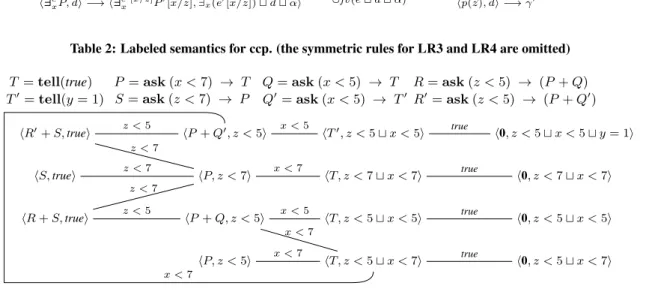
rules, except LR4, are easily seen to realize the above intuition. An explanation of LR5 is not needed to understand the present work. For the sake of space, we refer the reader to [1] for a more detailed explanation of these labeled rules. Fig. 1 illustrates the LTSs of our running example.
Syntactic Bisimilarity. When defining bisimilarity over a LTS, barbs are not usually needed because they can be somehow inferred from the labels of the transitions. For instance, in CCS, P ↓a iff
LR1htell(c), ditrue −→ h0, d ⊔ ci LR2 α ∈ min{a ∈ Con0| c ⊑ d ⊔ a } hask (c) → P, di−→ hP, d ⊔ αiα LR3 hP, di α −→ hP′, d′i hP k Q, di−→ hPα ′k Q, d′i LR4 hP, di α −→ hP′, d′i hP + Q, di−→ hPα ′, d′i LR5 hP [z/x], e[z/x] ⊔ di α −→ hP′, e′⊔ d ⊔ αi h∃exP, di α −→ h∃e′ [x/z]x P ′ [x/z], ∃x(e′[x/z]) ⊔ d ⊔ αi x 6∈ fv (e′), z 6∈ fv (P ) ∪fv (e ⊔ d ⊔ α) LR6 hP [~z/~x], di−→ γα ′ hp(~z), di−→ γα ′ for p(~x)def = P
Table 2: Labeled semantics for ccp. (the symmetric rules for LR3 and LR4 are omitted) T = tell(true) T′= tell(y = 1) P= ask (x < 7) → T S = ask (z < 7) → P Q= ask (x < 5) → T Q′= ask (x < 5) → T′ R= ask (z < 5) → (P + Q) R′= ask (z < 5) → (P + Q′) hR + S, truei hS, truei hR′+S, truei hP + Q′, z < 5i hP, z < 7i hP + Q, z < 5i hP, z < 5i hT′, z < 5⊔ x < 5i hT, z < 7 ⊔ x < 7i hT, z < 5 ⊔ x < 5i hT, z < 5 ⊔ x < 7i h0, z < 5 ⊔ x < 5 ⊔ y = 1i h0, z < 7 ⊔ x < 7i h0, z < 5 ⊔ x < 5i h0, z < 5 ⊔ x < 7i x < 7 z < 5 z < 7 z < 7 z < 5 z < 7 x < 5 x < 7 x < 5 x < 7 x < 7 true true true true
Figure 1: The labeled transition systems of the running example (IS={hR′+ S, truei, hS, truei, hR + S, truei}).
P −→. However this is not the case of ccp: barbs cannot be re-a moved from the definition of bisimilarity because they cannot be inferred from the transitions.
Taking into account the barbs, the obvious adaptation of labeled bisimilarity for ccp is the following:
Definition 4. [1] A syntactic bisimulation is a symmetric rela-tion R on configurarela-tions s.t. whenever (γ1, γ2)∈ R:
(i) if γ1↓cthen γ2↓c, (ii) if γ1 α −→ γ′ 1then ∃γ′2s.t. γ2 α −→ γ′ 2and (γ1′, γ2′)∈ R.
γ1and γ2are syntactically bisimilar, (γ1 ∼S γ2) if there exists a
syntactic bisimulation R s.t. (γ1, γ2)∈ R.
Unfortunately as shown in [1] ∼S is over-discriminating. As
an example, consider the configurations hP + Q, z < 5i and hP, z <5i, whose LTS is shown in Fig. 1. They are not equivalent according to ∼S. Indeed hP + Q, z < 5i
x<5
−→, while hP, z < 5i 6−→. However they are equivalent according to ˙x<5 ∼sb(Ex. 3).
3.
IRREDUNDANT BISIMILARITY
Syntactic bisimilarity is over-discriminating because of some re-dundant transitions. For instance, consider the transitions: (a) hP + Q, z < 5ix<7
−→ hT, z < 5 ⊔ x < 7i; (b) hP + Q, z < 5ix<5
−→ hT, z < 5 ⊔ x < 5i.
Transition (a) means that for all constraints e s.t. x < 7 ⊑ e, (c)hP + Q, z < 5 ⊔ ei −→ hT, z < 5 ⊔ ei, while transition (b) means that the reduction (c) is possible for all e s.t. x < 5 ⊑ e. Since x < 7 ⊑ x < 5, transition (b) is “redundant”, in the sense that its meaning is “logically derived” by transition (a).
The following notion captures the above intuition:
Definition 5. We say that hP, ci−→ hPα 1, c′i derives hP, ci β
−→ hP1, c′′i, written hP, ci−→ hPα 1, c′i ⊢D hP, ci
β
−→ hP1, c′′i, iff
there exists e s.t. the following conditions hold: (i) β = α ⊔ e (ii) c′′= c′
⊔ e (iii) α 6= β
One can verify in the above example that (a) ⊢D(b). Notice that
in order to check if hP + Q, z < 5i ˙∼sbhP, z < 5i, we could first
remove the redundant transition (b) and then check ∼S.
More generally, a naive approach to compute ˙∼sbwould be to
first remove all those transitions that can be derived by others, and then apply the partition refinement algorithm. However, this ap-proach would fail since it would distinguish hR + S, truei and hS, truei that, instead, are in ˙∼sb(Ex. 3). Indeed, hR + S, truei
can perform:
(e) hR + S, trueiz<7
−→ hP, z < 7i, (f) hR + S, truei−→ hP + Q, z < 5i,z<5
while hS, truei 6−→. Note that transition (f) cannot be derived byz<5 other transitions, since (e) 6⊢D(f). Indeed, P is syntactically
dif-ferent from P + Q, even if they have the same behaviour when inserted in the store z < 5, i.e., hP, z < 5i ˙∼sbhP + Q, z < 5i
(Ex. 3). The transition (f) is also “redundant”, since its behaviour “does not add anything” to the behaviour of (e).
Definition 6. Let R be a relation and γ → γα 1 and γ β
→ γ2be
two transitions. We say that the former dominates the latter one in R (written γ→ γα 1≻Rγ β → γ2) iff (i) γ α → γ1⊢Dγ β → γ′ 2 (ii) (γ′2, γ2)∈ R
A transition is redundant w.r.t. R if it is dominated in R by another transition. Otherwise, it is irredundant.
Note that the transition γ → γβ ′
2 might not be generated by the
rules in Tab. 2, but simply derived by γ α
P0 = {hR′ + S, truei, hS, truei, hR + S, truei}, {hP + Q′, z < 5i, hP + Q, z < 5i, hP, z < 5i}, {hP, z < 7i}, {hT ′, z < 5 ⊔ x < 5i, hT , z < 5 ⊔ x < 5i, h0, z < 5 ⊔ x < 5i}, {hT , z < 7 ⊔ x < 7i, h0, z < 7 ⊔ x < 7i}, {hT , z < 5 ⊔ x < 7i, h0, z < 5 ⊔ x < 7i}, {h0, z < 5 ⊔ x < 5 ⊔ y = 1i}
P1 = {hR′ + S, truei, hS, truei, hR + S, truei}, {hP + Q′, z < 5i, hP + Q, z < 5i, hP, z < 5i}, {hP, z < 7i}, {hT ′, z < 5 ⊔ x < 5i}, {hT , z < 5 ⊔ x < 5i}, {h0, z < 5 ⊔ x < 5i}, {hT , z < 7 ⊔ x < 7i}, {h0, z < 7 ⊔ x < 7i}, {hT , z < 5 ⊔ x < 7i}, {h0, z < 5 ⊔ x < 7i}, {h0, z < 5 ⊔ x < 5 ⊔ y = 1i} P2 = {hR′ + S, truei, hS, truei, hR + S, truei}, {hP + Q′, z < 5i}, {hP + Q, z < 5i, hP, z < 5i}, {hP, z < 7i}, {hT ′ , z < 5 ⊔ x < 5i}, {hT , z < 5 ⊔ x < 5i},
{h0, z < 5 ⊔ x < 5i}, {hT , z < 7 ⊔ x < 7i}, {h0, z < 7 ⊔ x < 7i}, {hT , z < 5 ⊔ x < 7i}, {h0, z < 5 ⊔ x < 7i}, {h0, z < 5 ⊔ x < 5 ⊔ y = 1i}
P3 = {hR′ + S, truei}, {hS, truei, hR + S, truei}, {hP + Q′, z < 5i}, {hP + Q, z < 5i, hP, z < 5i}, {hP, z < 7i}, {hT ′ , z < 5 ⊔ x < 5i}, {hT , z < 5 ⊔ x < 5i}, {h0, z < 5 ⊔ x < 5i}, {hT , z < 7 ⊔ x < 7i}, {h0, z < 7 ⊔ x < 7i}, {hT , z < 5 ⊔ x < 7i}, {h0, z < 5 ⊔ x < 7i}, {h0, z < 5 ⊔ x < 5 ⊔ y = 1i}
P4 = P3
Figure 2: The partitions computed by CCP-Partition-Refinement({hR′
+ S, truei, hS, truei, hR + S, truei}). instance, transition (e) dominates (f) in ˙∼sb, because (e) ⊢DhR +
S, truei−→ hP, z < 5i and hP, z < 5i ˙z<5 ∼sbhP + Q, z < 5i.
Therefore, we could compute ˙∼sb, by removing all those
transi-tions that are redundant wrt ˙∼sb. This, however, would lead us to
a circular situation: How to decide which transitions are redundant when redundancy itself depends on ˙∼sb.
Our solution relies on the following definition that allows to compute bisimilarity and redundancy at the same time.
Definition 7. An irredundant bisimulation is a symmetric rela-tion R on configurarela-tions s.t. whenever (γ1, γ2)∈ R:
(i) if γ1↓cthen γ2↓c,
(ii) if γ1−→ γα 1′is irredundant in R then ∃γ2′ s.t. γ2−→ γα 2′ and
(γ′
1, γ′2)∈ R.
γ1and γ2are irredundant bisimilar (γ1 ∼I γ2), if there exists an
irredundant bisimulation R s.t. (γ1, γ2) ∈ R.
Theorem 1. ∼I= ˙∼sb
PROOF. See [2].
4.
PARTITION REFINEMENT FOR CCP
Recall that we mentioned in Sec. 2 that checking ˙∼sbseems hard
because of the quantification over all possible constraints. How-ever, by using Theo. 1 we shall introduce an algorithm for checking
˙
∼sbby employing the notion of irredundant bisimulation.
The first novelty w.r.t. the standard partition refinement (Alg. 1) consists in using barbs. Since configurations satisfying different barbs are surely different, we can safely start with a partition that equates all and only those states satisfying the same barbs. Note that two configurations satisfy the same barbs iff they have the same store. Thus, we take as initial partition P0={IS⋆
d1} . . . {IS ⋆ dn},
where IS⋆
diis the subset of the configurations of IS
⋆with store d i.
Another difference is that instead of using the function F of Alg. 1, we refine the partitions by employing the function IR defined as follows: for all partitions P, γ1IR(P) γ2iff
• if γ1 α
−→ γ′
1 is irredundant in P, then there exists γ′2 s.t.
γ2 α
−→ γ′
2and γ1′Pγ′2.
It is now important to observe that in the computation of IR(Pn),
there might be involved also states that are not reachable from the initial states IS. For instance, consider the LTSs of hS, truei and hR + S, truei in Fig. 1. The state hP, z < 5i is not reachable but is needed to check if hR + S, truei−→ hP + Q, z < 5i is redundantz<5 (look at the example after Def. 6).
For this reason, we have also to change the initialization step of our algorithm, by including in the set IS⋆all the states that are
needed to check redundancy. This is done, by using the following closure rules. (IS) γ ∈ IS γ ∈ IS⋆ (RS) γ1∈ IS ⋆ γ1−→ γα 2 γ2∈ IS⋆ (RD) γ ∈ IS ⋆ γ−→ γα1 1 γ−→ γα2 2 γ−→ γα1 1⊢Dγ−→ γα2 3 γ3∈ IS⋆
The rule (RD) adds all the states that are needed to check redun-dancy. Indeed, if γ can perform both α1
−→ γ1 and α2 −→ γ2 s.t. γ −→ γα1 1 ⊢D γ α2 −→ γ3, then γ α2 −→ γ2 would be redundant whenever γ2∼˙sbγ3. Algorithm 2 CCP-Partition-Refinement(IS) Initialization
1. Compute IS⋆with the rules (
IS), (RS) and (RD), 2. P0:={IS⋆ d1} . . . {IS ⋆ dn}, IterationPn+1:= IR(Pn)
TerminationIf Pn=Pn+1then return Pn.
Fig. 2 shows the partitions computed by the algorithm with ini-tial states hR′
+ S, truei, hS, truei and hR + S, truei. Note that, as expected, in the final partition hR + S, truei and hS, truei be-long to the same block, while hR′+ S, truei belong to a
differ-ent one (meaning that the former two are saturated bisimilar, while hR′
+S, truei is different). In the initial partition all states with the same store are equated. In P1, the blocks are split by considering
the outgoing transitions: all the final states are distinguished (since they cannot perform any transitions) and hT′, z < 5
⊔ x < 5i is distinguished from hT, z < 5 ⊔ x < 5i. All the other blocks are not divided, since all the transitions with label x < 5 are redundant in P0(since hP, z < 5iP0hP + Q′
, z <5i, hP, z < 5iP0hP + Q,
z <5i and hT′, z <5
⊔ x < 5iP0hT, z < 5 ⊔ x < 5i). Then, in P2, hP + Q′, z < 5i is distinguished from hP, z < 5i since
the transition hP + Q′
, z < 5i −→ is not redundant anymore inx<5 P1(since hT′
, z <5⊔ x < 5i and hT, z < 5 ⊔ x < 5i belong to different blocks in P1). Then in P3, hR′+ S, truei is
distin-guished from hS, truei since the transition hR′+ S, truei−→ isx<5
not redundant in P2 (since hP + Q′
, z <5i 6P2hP, z < 5i).
Fi-nally, the algorithm computes P4that is equal to P3and return it.
It is interesting to observe that the transition hR + S, truei x<5
−→ is redundant in all the partitions computed by the algorithm (and thus in ˙∼sb), while the transition hR′+ S, truei
x<5
−→ is considered redundant in P0and P1and not redundant in P2and P3.
4.1
Termination
Note that any iteration splits blocks and never fuse them. For this reason if IS⋆is finite, the algorithm terminates in at most |IS⋆|
iterations. The proof of the next proposition assumes that ⊢Dis
de-cidable. However, as we shall prove in the next section, the decid-ability of ⊢Dfollows from our assumption about the decidability
of the ordering relation ⊑ of the underlying constraint system and Theo. 3 in the next section.
Proposition 2. If IS⋆is finite, then the algorithm terminates and the resulting partition coincides with ˙∼sb.
PROOF. See [2].
We now prove that if the set Config(IS) of all configurations reachable from IS (through the LTS generated by the rules in Tab. 2) is finite, then IS⋆is finite.
This condition can be easily guaranteed by imposing some syn-tactic restrictions on ccp terms, like for instance, by excluding ei-ther the procedure call or the hiding operator.
Theorem 2. If Config(IS) is finite, then IS⋆is finite. PROOF. See [2].
4.2
Complexity of the Implementation
Here we give asymptotic bounds for the execution time of Alg. 2. We assume that the reader is familiar with the O(.) notation for asymptotic upper bounds in analysis of algorithms–see [6].
Our implementation of Alg. 2 is a variant of the original parti-tion refinement algorithm in [10] with two main differences: The computation of IS⋆according to rules (
IS), (RS) and (RD) (line 2,
Alg. 2) and the decision procedure for ⊢D (Def. 5) needed in the
redundancy checks.
Recall that we assume ⊑ to be decidable. Notice that require-ment of having some e that satisfies both conditions (i) and (ii) in Def. 5 suggests that deciding whether two given transitions belong to ⊢Dmay be costly. The following theorem, however, provides a
simpler characterization of ⊢Dallowing us to reduce the decision
problem of ⊢Dto that of ⊑.
Theorem 3. hP, ci−→ hPα 1, c′i ⊢DhP, ci β
−→ hP1, c′′i iff the
following conditions hold: (a) α < β (b) c′′= c′⊔ β
PROOF. See [2].
Henceforth we shall assume that given a constraint system C, the function fCrepresents the time complexity of deciding (whether
two given constraints are in) ⊑. The following is a useful corollary of the above theorem.
Corollary 1. Given two transitions t and t′, deciding whether t⊢Dt′takes O(fC) time.
Remark 2. We introduced ⊢Das in Def. 5 as natural adaptation
of the corresponding notion in [5]. The simpler characterization given by the above theorem is due to particular properties of ccp transitions, in particular monotonicity of the store, and hence it may not hold in a more general scenario.
Complexity.The size of the set IS∗is central to the complexity
of Alg. 2 and depends on topology of the underlying transition graph. For tree-like topologies, a typical representation of many transition graphs, one can show by using a simple combinatorial argument that the size of IS∗is quadratic w.r.t. the size of the set of
reachable configurations from IS, i.e., Config(IS). For arbitrary graphs, however, the size of IS∗may be exponential in the number
of transitions between the states of Config(IS) as shown by the following construction.
Definition 8. Let P0 = 0 and P1 = P. Given an even number
n, define sn(n, 0) = 0, sn(n, 1) = ask (true) → sn(n, 0) and
for each 0 ≤ i < n ∧ 0 ≤ j ≤ 1 let sn(i, j) = (ask (true) →
sn(i, j⊕ 1)j⊕1 + (ask (bi,j) → 0) + (ask (ai) → sn(i + 1,
j)) where⊕ means addition modulo 2. We also assume that (1) for each i, j : ai <bi,jand (2) for each two different i and i′ : ai 6⊑
ai′,and (3) for each two different (i, j) and (i′, j′): bi,j6⊑ bi′,j′.
Let IS = {sn(0, 0)}. One can verify that the size of IS∗is
in-deed exponential in the number of transitions between the states of Config(IS).
Since Alg. 2 computes IS∗the above construction shows that
on some inputs Alg. 2 take at least exponential time. We conclude by stating an upper-bound on the execution time of Alg. 2.
Theorem 4. Let n be the size of the set of states Config(IS) and let m be the number of transitions between those states. Then n× 2O(m)× fCis an upper bound for the running time of Alg. 2.
PROOF. See [2].
5.
CONCLUDING REMARKS
In this paper we provided an algorithm for verifying (strong) bisimilarity for ccp by building upon the work in [5]. Weak bisimi-larity is the variant obtained by ignoring, as much as possible, silent transitions (transitions labelled with true in the ccp case). Neither [5] nor the present work deal with this weak variant. We therefore plan to provide an algorithm for this central equivalence in future work.
6.
REFERENCES
[1] A. Aristizabal, F. Bonchi, C. Palamidessi, L. Pino, and F. D. Valencia. Deriving labels and bisimilarity for concurrent constraint programming. In FOSSACS, pages 138–152, 2011. [2] A. Aristizabal, F. Bonchi, L. Pino, and F. Valencia. Partition
refinement for bisimilarity in ccp (extended version). Technical report, INRIA-CNRS, 2012. Available at: http://www.lix.polytechnique.fr/~andresaristi/sac2012.pdf. [3] F. Bonchi, F. Gadducci, and G. V. Monreale. Reactive
systems, barbed semantics, and the mobile ambients. In FOSSACS, pages 272–287, 2009.
[4] F. Bonchi, B. König, and U. Montanari. Saturated semantics for reactive systems. In LICS, pages 69–80, 2006.
[5] F. Bonchi and U. Montanari. Minimization algorithm for symbolic bisimilarity. In ESOP, pages 267–284, 2009. [6] T. H. Cormen, C. E. Leiserson, R. L. Rivest, and C. Stein.
Introduction to Algorithms (3. ed.). MIT Press, 2009. [7] F. S. de Boer, A. D. Pierro, and C. Palamidessi.
Nondeterminism and infinite computations in constraint programming. Theor. Comput. Sci., 151(1):37–78, 1995. [8] J.-C. Fernandez. An implementation of an efficient algorithm
for bisimulation equivalence. Sci. Comput. Program., 13(1):219–236, 1989.
[9] G. Ferrari, S. Gnesi, U. Montanari, M. Pistore, and G. Ristori. Verifying mobile processes in the hal environment. In CAV, pages 511–515, 1998.
[10] P. C. Kanellakis and S. A. Smolka. Ccs expressions, finite state processes, and three problems of equivalence. In PODC, pages 228–240, 1983.
[11] R. Milner and D. Sangiorgi. Barbed bisimulation. In ICALP, pages 685–695, 1992.
[12] U. Montanari and V. Sassone. Dynamic congruence vs. progressing bisimulation for ccs. FI, 16(1):171–199, 1992. [13] V. A. Saraswat and M. C. Rinard. Concurrent constraint
programming. In POPL, pages 232–245, 1990.
[14] V. A. Saraswat, M. C. Rinard, and P. Panangaden. Semantic foundations of concurrent constraint programming. In POPL, pages 333–352, 1991.
[15] B. Victor and F. Moller. The mobility workbench - a tool for the pi-calculus. In CAV, pages 428–440, 1994.