Abstract— This paper presents a comparison of optimization
algorithms for constrained damping (CLD) patches’ layout to minimize the maximum vibration response of the odd modes, which constitutes the dominant acoustic radiation, of a simply-supported beam excited by a harmonic transverse force. An analytical model based on Euler-Bernoulli beam assumptions is derived first to relate the displacement response of the beam with bonded CLD patches and their layout. Four different nonlinear optimization methods/algorithms are then respectively used to optimize the CLD patches’ locations and lengths with aim of minimum displacement amplitude at middle of the beam. The considered methods include subproblem approximation method, the first-order method, sequential quadratic programming (SQP) and genetic algorithm (GA). The efficiency of each considered optimization method is evaluated and also compared in terms of obtained optimal beam displacement. The results show that GA is most efficient in obtaining the best optimum for this optimization problem in spite of highest computation efforts required to improve its stability.
Key words— Constrained Layer Damping; Nonlinear optimization; Vibration control; comparative study.
I. I
NTRODUCTIONt is well-known that constrained layer damping (CLD) is the effective means for suppressing the structural vibration and noise radiation. It the past decades, there have been numerous papers published in the area of CLD treatment. Earlier works on CLD are mainly on passive constrained layer damping (PCLD). The theoretical work could be traced to DiTaranto [1] and Mead and Markus [2] for the axial and bending vibration of sandwiched beams. After that, different formulations and techniques for modeling and predicting the energy-dissipation of the viscoelastic core layer when the PCLD-treated structure is in vibrating [3~5] have been reported. This was followed by a number of more comprehensive formulations, for example, inclusion of thickness deformation of the core layer in the model [6] and dealing with cases where only a portion of the base structure is covered with PCLD [7], by various authors to characterize the PCLD treatment. Since 1970’s, finite element procedure has
been adopted in modeling layer damping for vibration control of complex structures [8,9].
By 1990's, active constrained layer damping (ACLD) has begun to receive much attention. The ACLD configuration uses an active element, usually a piezoelectric layer, to replace or augment the passive constraining layer, thereby enhancing the energy dissipation of the damping. Several analytical formulations of ACLD treatments were then proposed. Among those, the mathematical models by Baz and Ro [10], and Shen [11] are most widely used. Baz derived a sixth order ordinary differential equation governing bending vibration control of an Euler-Bernoulli beam with full and partial ACLD treatment while Shen's mathematical model addresses the coupling nature of the bending and axial motions of an Euler-Bernoulli beam with ACLD treatments. More recently, Huang et al [12] and later Gao & Shen [13] used the assumed-modes method and closed loop velocity feedback control law to arrive at the equations of motion governing the vibration of a cantilever beam with partially treated self-sensing ACLD patch. Various analytical and numerical analyses were then performed based on these models. The feasibility and performance of ACLD treatment were also experimentally determined [14,15].
Extensive efforts have also been exerted to optimally design passive and active constrained layer damping treatments of vibrating structures. These efforts aim to maximize the modal damping ratios and modal strain energies by determining the optimal material and geometric parameters of the treatments, or minimize weight by selecting the optimal length and location. For example, Baz and Ro [10] used Univariate Search Method (USM) to optimize the performance of the ACLD treatments by selecting the optimal thickness and shear modulus of the viscoelastic layer as well as the control gain for fully-treated beam when proportional and derivative controllers are used. Marcelin et al [16,17] used genetic algorithm and beam finite elements to maximize the damping factor for partially-treated beam. The design variables were the dimensions and locations of the patches. As verified by Nokes and Nelson [18], this layout optimization of CLD patches can lead to significant saving in the amount of ACLD material used.
Mathematically, the layout optimization of CLD patches may be defined as a nonlinear optimization problem as: Find design variables, patch lengths and locations, to minimize an objective function, the vibration response of CLD-treated structure, subjected to an inequality constraint of allowed added weight of CLD treatment. There have been a number of optimization algorithms/methods available to solve this problem. Undoubtedly, the optimization method to be used
I
A Comparative Study on Optimization of Constrained Layer
Damping for Vibration Control of Beams
G. S. H. Pau
a), H. Zheng
b)AND G. R. Liu
a)Manuscript received November 1, 2002. G.R. Liu and G.S.H. Pau are from Singapore-MIT Alliance, The National University of Singapore, 10 Kent Ridge Crescent, Singapore 119260. H. Zheng is from Institute of High Performance Computing, 1 Science Park Road, #01-01 The Capricorn, Singapore Science Park II, Singapore 117528 (e-mail: [email protected]).
relies heavily on the nature of the problem being optimized. Most existing optimization algorithms are designed to find a local optimum. One example is the sequential quadratic programming (SQP) algorithm [19] which has shown to be robust and efficient for most optimization problems. However, to the designers, it is often of interest to find the best optimum in the whole feasible design space. Since no mathematical conditions for global optimality exist, a global optimum is usually much more difficult to find than a local optimum. Some methods have therefore been developed to find an approximation of the global optimum without searching the whole feasible design domain. The genetic algorithm (GA) is an example of such methods [20,21]. Although its basic ideas of analysis and design were initially based on the concepts of biological evolution, the GA has been used to solve various optimization problems in engineering practices.
The main objective of this study is to look for an optimization algorithm/method which is most suitable for solving the CLD layout optimization problem. The study consists of two parts. In the first part, a semi-analytical model as proposed by Huang et al [12] and Gao & Shen [13] is developed for displacement response of beams with bonded multiple ACLD patches, instead of using finite elements formulation used by Baz & Ro [10,15] and Marcelin et al [16,17]. The purpose of doing this is to relate the objective function to be optimized and the design variables, i.e., the locations and lengths of patches. In the second part, several available optimization algorithms are respectively applied to solve the problem of CLD patches layout optimization. It is assumed that the physical and geometrical properties of all the layers are known except the locations and lengths of the patches. The optimal design entails finding a patch layout to provide maximum vibration attenuation. These optimization algorithms are then evaluated through comparing their performance in terms of obtained optima and computation efforts required.
The paper looks at four optimization methods, namely (1) subproblem approximation method, (2) the first order optimization method, (3) sequential quadratic programming algorithm, and (4) a genetic algorithm. Comparison of these methods is preceded by a description of the analytical model used in the numerical simulation of the vibration of a simply-supported beam.
II. MATHEMATICAL MODEL OF BEAM WITH CLD
TREATMENT
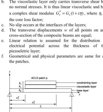
A beam with partial CLD treatment is modeled as a composite beam consisting of three layers, namely the base, constraining and viscoelastic layers, denoted by the subscripts/superscripts b, c and v respectively. The general configuration is shown in Fig. 1 for a simply-supported beam treated with a CLD patch p and the labeled various design parameters and design variables. The constraining layer is the elastic layer for PCLD treatment or piezoelectric layer for ACLD treatment. All layers have the same width b but
different thickness denoted by hi, where i = b, c or v.
Similarly, Yi is elastic modulus of the ith layer. Following
assumptions are made [10~13]:
a. Shear strains in the piezoelectric layer and the base layer are negligible;
b. The viscoelastic layer only carries transverse shear but no normal stresses. It is thus linear viscoelastic and has a complex shear modulus Gv* =Gv(1+iη), where ηv is
the core loss factor;
c. No slip occurs at the interfaces of the layers;
d. The transverse displacements w of all points on any cross-section of the composite beams are equal;
e. Linear relation is assumed for the distribution of electrical potential across the thickness of the piezoeletric layer;
f. Geometrical and physical parameters are same for all the patches.
Fig. 1 A simply-supported beam with 1 partial ACLD patch p
A. Kinematic relation
It is assumed that the continuity of displacement at the interface between the layers is as shown in Fig. 2. This assumption requires that the following relations hold [12]:
∂ ∂ − − = ∂ ∂ − ∂ ∂ − + = ∂ ∂ + x w h u x w h u x w h u x w h u v v v b b v v v c c γ γ 2 2 2 2 (1)
where uc, uv and ub are respectively the mid-plane
displacements of the constraining layer, viscoelastic layer and base layer along the x-axis. γv is the rotation of the normal to
the mid-plane of the viscoelastic layer. The strain-displacement relations for the base and the piezoeletric layer can be expressed as follows based on the classic beam theory:
2 2 2 2 x w z x u x w z x u b b c c ∂ ∂ − ∂ ∂ = ∂ ∂ − ∂ ∂ = ε ε (2) where ui is the mid-plane displacements of the ith layer, and x
is the axial distance relative to one end of the beam.
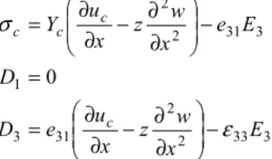
Then, by considering only the poling direction (since the piezoelectric layer is thinner than the base layer), it is found that E3 = E3 (x, t) and E1 = 0, where E is the electric field
= 0. Thus, the one-dimensional constitutive equations for the piezoeletric material are given by:
3 33 2 2 31 3 1 3 31 2 2 0 E x w z x u e D D E e x w z x u Y c c c c ε σ − ∂ ∂ − ∂ ∂ = = − ∂ ∂ − ∂ ∂ = (3)
where D the electric displacement, e31 the piezoelectric
coefficient and ε33 the dielectric constant. In addition, by
considering the longitudinal equilibrium of the base layer and continuity of displacement at the interfaces, following relations can be obtained:
(
c b)
v b v b b v b c h h h h x u G Y h h x w h u u + + = ∂ ∂ + ∂ ∂ − = 2 1 2 2 * (4)Fig. 2 The deformation pattern of the layers in the model of beam with CLD treatment
B. Energy expressions
The above relations are then used to derive the expression of the potential energies of the layers and kinetic energy of the beam. For the case of multiple patches, the potential energy of the piezoelectric layer consists of strain energy and electric energy as:
∑∫
∑
∫
∫
= = ∂ ∂ + − ∂ ∂ − ∂ ∂ + ∂ ∂ = − = p p p p n p x x c c c c n p c c c c c V V c c c dx x u E e E bh dx x u E be h x w I Y x u A Y dv E D dv V 1 3 31 2 3 33 3 31 1 2 2 2 2 3 3 2 1 2 1 2 1 2 1 2 1 ε ε σ (5)where np is total number of patches for the treatment. The
potential energy of the base layer is simply its strain energy:
∫
∫
∂ ∂ + ∂ ∂ = = L b b b b b V b b b dx x w I Y x u A Y dv V 0 2 2 2 2 2 1 2 1 ε σ (6)The potential energy of the viscoelastic layer is
∑∫
∑∫
= = ∂ ∂ = = p p p p p p n p x x b v b b v n p x x v v v v dx x u G Y h A dx A G V 1 2 2 * 2 2 1 2 * 2 1 2 1 2 1 2 1 γ (7)and the kinetic energy for the whole beam is
(
)
∑
∫
∫
= ∂ ∂ + ∂ ∂ + = np p L b b x x c c v v t dx w A dx t w A A T p p 1 0 2 2 2 1 2 1 ρ ρ ρ (8)Assuming an external transverse load of f(x, t), actuation voltage of V(x, t) applied to the piezoeletric layer and a charge density of Q(x, t), the work done by these forces can be expressed as:
( ) ( )
( ) ( )
( ) ( )
∑∫
∑∫
∫
= = = = = p p p p p p n p x x c n p x x L dx t x Q t x E bh dx t x Q t x bV P dw t x w t x f P 1 3 1 2 0 1 2 1 2 1 , , , , , , (9) C. Equation of motionSemi-analytical approach is used to derive the equation of motion. The displacement is thus approximated by assumed-modes expansion. For a beam, the displacement is given by:
( )
( ) ( )
( )
( ) ( )
ξ ξ η η T n i i i b T n i i i U t x U t x u W t x W t x w = = = =∑
∑
= = 1 1 , , (10)where W and U are the transverse and longitudinal mode shape functions of the beam while η and ξ are the generalized coordinates according to transverse and longitudinal displacements, respectively. In this study, the setting used consists of a simply-supported beam, excited harmonically by a point disturbance of unity amplitude at the middle of the beam. Thus, the mode shape functions are [22]
( )
( )
= = L x i x U L x i x W i i π π cos sin (11) Then, by substituting the related equations into the extended Hamilton’s principle, i.e.(
)
[
]
∫
2 − + + + + = 1 0 2 1 t t T Vc Vv Vb P P dt δ (12)using a velocity feedback control law where dt dE G E v 0 3 3 =− (13) and the sensed voltage by piezoelectric film sensor given by
∂ ∂ + ∂ ∂ − ∂ ∂ − = 2 1 33 2 33 31 0 3 x u G x w h x u e E b b ε (14)
the governing equations of the motion can be derived as follows [13]:
( )
= + + ∫
0 , 2 1 0 0 0 0 22 21 12 11 22 21 12 11 11 L idx W t x f K K K K C C C C M ξ η ξ η ξ η & & && && (15) where(
)
(
)
(
)
(
[
)
]
(
)
(
)
* 2 2 2 * 1 2 1 1 1 33 2 31 22 12 21 1 1 33 2 31 12 1 33 2 2 31 11 0 2 1 1 1 2 22 12 21 1 1 12 0 1 2 11 0 1 11 , 2 2 2 1 2 1 2 1 2 1 2 1 2 1 2 1 G Y h A G G Y h h G dx U U G U U G U U G E e A C C C dx W U G W U G E h e A C dx W W G E h e A C dx U U I Y dx U U G U U G U U A Y U U G K K K dx W U G W U h A Y K dx W W I Y dx W W h A Y I Y K dx WW A dx WW A A M b b v b b v T T np p x x T v c T np p x x T v c np p x x T v c L T b b T T np p x x T c c T n p x x T T c c L T b b n p x x T c c c c L T b b n p x x T v v c c p p p p p p p p p p p p p p p p p = = ′′′ ′′′ + ′′′ ′ + ′ ′ − = = ′′ ′′′ + ′′ ′ = ′′ ′′ − = ′ ′ + ′′′ ′′′ + ′′′ ′ + ′ ′ + ′′ ′′ = = ′′ ′′′ + ′′ ′ − = ′′ ′′ + ′′ ′′ + = + + =∑∫
∑∫
∑∫
∫
∑∫
∑∫
∫
∑∫
∫
∑∫
= = = = = = = ρ ρ ρFor the case of PCLD treatment, Cij (i,j=1,2) in the system
equation (15) are equal to zero since no voltage is applied to the constraining layer. Solving this system equation yields the solution of displacement at any beam location. As our objective of optimization is to find the optimal layout of the CLD patches aiming to maximizing the vibration attenuation
of the odd modes, the main objective function is the amplitude at the middle of the beam:
Objective function
∑
= = n i i L W 1 2 (16)There is also a secondary objective function of minimizing the total weight of the CLD patches used. A frequency range from 0Hz to 3.5kHz is considered, which covers the lowest three odd modes of transverse vibration.
III. Subproblem Approximation Method and First Order Optimization Method
A. Description of methods
Two early methods, namely the subproblem approximation method and first order optimization method, are investigated first. These two methods are chosen for evaluation because they have already been integrated into a multi-physics commercial finite element code, ANSYS, as optimization tools [23]. In these two methods, a constrained problem is formulated into a basic unconstrained problem by using a penalty function for solutions which are near or beyond the constraint boundary. The constrained problem is then solved using a sequence of parameterized unconstrained optimizations, which in the limit (of the sequence) converges to the constrained problem.
In subproblem approximation method, the objective function and the constraints are first being approximated using least squares fitting of a number of design sets generated randomly. The constrained minimization problem is then converted into an unconstrained form by using penalty functions, leading to the following subproblem statement:
(
)
( )
( )
( )
+ + + =∑
∑
∑
= = = 2 1 1 1 1 0 ˆ ˆ ˆ , m i i m i i n i i k k f f p X x Gg Hh p x F (17)in which fˆ , gˆ and hˆ are the objective function, inequality constraints and equality constraints respectively, and X, G and
H are the penalty functions used to enforce the constraints. f0
is introduced to achieve consistent units while pk is a response
surface parameter which increases with each design iteration in order to achieve accurate, converged result. A sequential unconstrained minimization technique is then used to solve each design iteration. The algorithm is terminated when convergence occurs or maximum number of iterations is reached.
In first order optimization method, instead of using least-squares fitting, the constrained problem is directly transformed into an unconstrained form, using the following formulation:
( )
∑
( )
∑
( )
∑
( )
= = = + + + = n i m i m i i h i g i x x q P g P h P f f q x Q 1 1 1 0 1 2 , (18)where Px, Pg and Ph are the exterior penalty function of the
objective function and constraints. Gradient method utilizing various steepest descent and conjugate direction searches are then performed during each iteration until convergence is
reached. More theoretical details of the two methods have been given in [19].
B. Results and discussion
The beam used for the optimization study has simply-supported boundary condition. Its geometric parameters are a length of 0.4 m, a width of 0.03 m and a thickness of 0.004 m. The geometric and material properties used for the study are shown in Table 1 with inclusion of physical parameters of PCLD patches for damping treatment. The loss factor of the viscoelastic core is set at a desired maximum value and is invariant with respect to frequency. In addition, a structural damping is introduced in the form of a complex Elastic Modulus for both beam and constraining layer, given by
) 1 ( ~ η i E E= + where η is the structural loss factor.
TABLE 1
PROPERTIES OF MATERIALS USED IN ANALYSIS OF BEAM
Properties (aluminium) Beam PZT material (PZT-5H) Viscoelastic material
Elastic Modulus, E~(GPa) 70(1 + 0.0001i) 49(1 + 0.0001i) − Density, ρ (kg/m3) 2.71 × 10³ 7.50 × 10³ 1.00 × 10³ Thickness, h (m) 0.004 0.002 0.001 Shear Modulus, G (MPa) − − 0.896(1 + 0.5i)
A general configuration for the layout of the patches is then proposed to reduce the number of variables. For a general
np-CLD configuration where np is the number of CLD patches,
np, is always restricted to odd numbers in this optimization
study. Then, the centers of these np patches are aligned to np
locations evenly spaced along the beam. Theoretically, this arrangement gives the greatest effect in damping out the odd modes since the patches are placed at the peaks of the odd modes.
Secondly, let the middle position of the beam be x = 0. Then the patches at -x and x are of same length based on the symmetric property of odd modes. The layout is illustrated in Fig. 3 for a 5-CLD configuration.
Fig. 3 A 5-CLD configuration
We begin with the optimization of a 1-CLD treatment of the beam. The resulting frequency response of such a configuration is compared to the response of a plain beam. As the amplitude at the center of the beam is examined, the peaks
in the frequency response plot belong to odd modes of the beam vibration.
The objective function consists of two components, i.e. the amplitude at the center of the beam and the total length of the CLD patches, ltotal. Thus, the design variable in this
optimization problem for a 1-CLD configuration is the patch's length since the amplitude of the vibration is a function of the patch's length. However, the magnitudes of the two components of the objective function are of very different orders. To avoid the patch's length from dominating the objective function, it is multiplied by a factor of 10-5. In
addition, an arbitrary weight factor of 0.1 is assigned to the patch's length as well. Let f(ltotal) be the function which returns
the amplitude at the center of the beam. Then the objective function is given by
minimize f
( )
ltotal +10−6ltotalThe objective function is minimized over the frequency range of 0-3000 Hz by optimization methods. This yields an optimal length of 0.195 m. As can be seen in Fig. 4, the optimized solution leads to large vibration attenuation, namely 16.62 dB, 28.39 dB and 46.20 dB for the first 3 odd modes. The overall reduction over the frequency range of 0-3000 Hz is 16.62 dB. However, the length of the CLD patch is 0.195 m, which is an added weight of 72%.
Fig. 4 Frequency response of the beam with PCLD treatment using single patch
When the optimization is performed for a 3-CLD configuration using a similar objective function, the overall reduction achieved in the frequency range 0-3000 Hz by subspace approximation method and first order method are 24.79 dB and 18.91 dB respectively. The resulting frequency responses are shown in Fig. 5 and optimized total lengths of 0.197 m (72.7% added weight) and 0.17 m (62.7% added weight) are obtained respectively. Clearly, the percentage of added weight is still very high. This is because we have not found a global minimum. The design space of the optimization problem for the 3-CLD configuration is nonlinear and nonconvex, as shown in Fig. 6. Although penalty function
method is a nonlinear optimization method, it is only capable of finding a local minimum. Thus, attainment of a global minimum is not guaranteed in both methods considered.
Fig. 5 Frequency response of the beam with PCLD treatment using 3 patches
Fig. 6 Maximum displacement at x = 0.2 m versus ratio of the mid CLD patch to total length of the CLD patches for a total CLD coverage of 18.45% added weight
IV. SEQUENTIAL QUADRATIC PROGRAMMING
A. Description of method
Sequential quadratic programming (SQP) is a widely-used method for most optimization problems owing to its robustness and high efficiency in searching for the optimum. Although it is also a penalty method as above two methods, it is exact in the sense that it requires only one unconstrained minimization to obtain an optimal solution of the original constrained problem. Considering a general problem of minimize f(x), subject to g(x) ≤ 0, we can write the Lagrangian function as [19]
( ) ( )
∑
( )
= + = m i i ig x x f x L 1 ,λ λ (19) where λi is the Lagrangian multiplier. Then the quadraticprogramming (QP) subproblem can be formulated based on a quadratic approximation of the Lagrangian function:
( )
( )
( )
( )
( )
0 0 subject to 2 1 min ≤ + ∇ = + ∇ + ∈ k i T k i k i T k i T k k T R d x g d x g x g d x g d x f d H d n δ (20) The matrix Hk is a positive definite approximation of theHessian matrix of the Lagrangian function and can be updated by using quasi-Newton methods. The solution to the subproblem is then used to form a new iterate until convergence occurs.
To improve the chances of obtaining a minimum closer to global minimum, a trial-and-error or heuristic approach is used together with the SQP method. A simple heuristic method involves randomly selecting a set of starting points in the hope that one of these starting points is close to the global minimum. While global minimum is not assured, the probability of obtaining a better minimum increases with number of starting points.
B. Results and discussion
The problem formulation in Section 3.2 cannot provides meaningful comparison between the methods because both components in the objective function may vary and the solution is subjected to the weightage assigned to each component. We also need to analyze the influence of the total amount of CLD material used on the layout and the frequency response of the PCLD treatment. Thus, we take another approach in which the total amount of CLD material is subjected to an equality constraint. The total length of the CLD patch is then fixed for each optimization run. Let f(y) be a function which returns the maximum displacement in a desired frequency range given a total length of CLD patches,
ltotal and yk is the ratio of individual patch length, lk, to ltotal
where k = 1, …, ½ (n+1). Our optimization problem can then be formulated as follows: maximize f(y) 2 1 , , 1 , 0 , constant 1 2 2 1 , , 1 , 1 2 1 subject to 2 / ) 1 ( 1 2 / ) 1 ( 2 1 + = ≥ = + ≤ − = + ≤ + = + + + + =
∑
n k l y l n y n k n y y y y total k total n k k n k k L L (21)To compare the current SQP-heuristic method with above two penalty methods, we optimize the 3-CLD configuration with the total length of patches fixed at 0.17 m (62.7% added weight). A maximum displacement of 1.6116 ×10⁻⁴ is obtained
for the frequency range 0-3000 Hz and this is equivalent to a reduction of 24.50 dB. Compared to 18.91 dB obtained using the first order method, this is a further reduction of 29.6%. The computing resources required by SQP-heuristic method is also significantly less than ANSYS implementation of penalty method.
For a 5-CLD configuration, the maximum displacements of the optimal layout (found through SQP-heuristic method) for different ltotal are plotted against the percentage of added
weight as shown in Fig. 7. The layout is separately optimized for mode 1, 3, 5 and 7. The resulting plots are irregular because the method fails to consistently achieve a global minimum. The configuration for the first two local minimums of the plot for mode 1 in Fig. 7 are used as basis for our possible optimal configurations as shown in Table 2.
Fig. 7 Amplitude versus % weight added with optimization performed over frequency ranges centered around four different odd modes
TABLE 2
TWO POSSIBLE OPTIMAL CLD CONFIGURATIONS
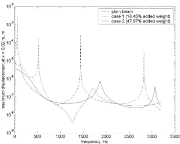
% weight added ltotal l1 l2 l3 maximum displacement 0 0 0 0 0 0 2.71 × 10⁻³ 1 18.45 0.05 0.0119 0.0117 0.0073 7.24 × 10⁻⁶ 2 47.97 0.13 0.0040 0.0562 0.0067 3.57 × 10⁻⁶ Fig. 8 shows the frequency response of the two optimal configurations described in Table 2. The vibration attenuations achieved across the frequency range of 0-3k Hz are 51.44 dB for case 1 and 57.66 dB for case 2. Compared to the previous results, it can be concluded that higher level of vibration attenuation is achieved with much lesser amount of patches.
Fig. 8 Frequency response for case 1 and case 2
V. GENETIC ALGORITHM
A. Description of method
Genetic algorithms is a more advanced heuristic method than the sampling method used in previous sections. It maintains and manipulates a family or population, of solutions and implements a simulated evolution or “survival of the fittest” strategy in their search for better solutions. In general, the fittest individuals of any population tend to reproduce and survive to the next generation, thus improving successive generations. GA has been shown to solve linear and nonlinear problems by exploiting all regions of the state space and exponentially exploiting promising areas through mutation, crossover and selection operation applied to individuals in the population.
The current GA implementation utilizes the Genetic Algorithm Optimization Toolbox (GAOT) for MATLAB developed by Houck et al [24]. GAOT is designed for unconstrained problem. The layout optimization problem is however subjected to physical feasibility constraints, and constraints on the length of the patches. This constrained problem is converted into an unconstrained form by using penalty functions. Two forms of penalty functions are considered, namely penalty function with constant penalty factor and penalty function with penalty factor that increases with number of generations. Our preliminary analysis however showed no significant difference between the two.
B. Results and discussion
The same problem formulation of the 5-CLD configuration used in Section 4.2 is used and a total patch length of 0.05 m is considered. The optimal configuration obtained is l1 = 0.011 m, l2 = 0.0068 m and l3 = 0.013 m. The
resulting maximum displacement is 6.5086 ×10⁻⁶ m, which is
equivalent to a vibration reduction of 52.38 dB for the frequency range 0-3000 Hz. When the position of each patch
is relaxed and allowed to vary, the resulting maximum displacement obtained is only 1.2465 ×10⁻⁶ m, which is a
further reduction of 14.35 dB compared to the previous case. The configuration obtained is shown in Table 3. Comparison between the frequency response of the optimal configurations obtained using GAs and the plain beam is shown in Fig. 9.
TABLE 3
PARAMETERS IN THE 5-CLD CONFIGURATIONS OPTIMIZED USING GAS WITHOUT CONSTRAINTS ON POSITIONS OF THE PATCHES
Patch number position, m length, m
1 0.3859 0.01138
2 0.3100 0.004217
3 0.2680 0.0001463
4 0.1258 0.01320
5 0.3518 0.01498
Fig. 9 Frequency response for optimal configurations obtained using GAs for 18.45% added weight
VI. SUMMARY AND CONCLUSION
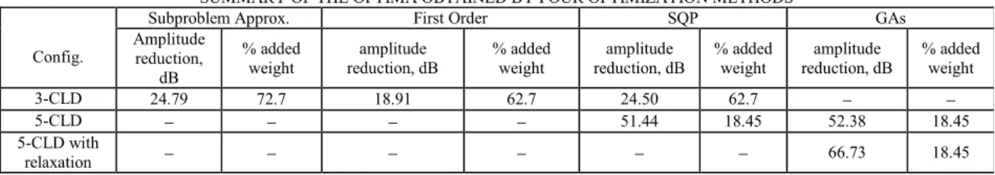
As a summary, the achieved optima of the structural volume displacement (SVD) reductions by the four optimization methods/algorithms respectively are given in
Table 4 with the percentage added weight included. In the column for “configuration”, “5-CLD with relaxation” means that the positions of the patches are treated as design variables. It can be easily seen that genetic algorithms (GAs) proves to be the best optimization method for our PCLD layout optimization problem among the methods considered. Large reduction in the amplitude is obtained with small percentage of added weight. In addition, GAs is able to handle large number of variables. Nevertheless, the computation efforts required are higher and consistent results cannot be obtained. The stability and reliability of the GA method can however be improved with increasing number of runs, as is done in the SQP-heuristic method.
Amongst the three local optimum searching methods, SQP can obtain similar optimum of SVD reduction under same constraint of percentage added weight as that by GAs, provided the positions of the patches be fixed in order to reduce the number of design variables to be optimized. Subproblem approximation method and the first order method behave similarly in solving the optimization problem of finding the optimal PCLD layout for noise reduction of vibrating beams.
REFERENCE
1. R.A. DiTaranto, 1965, Theory of vibratory bending for elastic and viscoelastic layered finite-length beams. ASME Journal of Applied Mechanics, 32: 881-886.
2. D.J. Mead and S. Markus, 1969, The forced vibration of a three-layer, damped sandwich beam with arbitrary boundary conditions. AIAA Journal, 10: 163-175.
3. K. Rao, 1978, Frequency and loss factors of sandwich beams under various boundary conditions. International Journal of Mechanical Engineering Science, 20: 271-278
4. M.J. Yan & E.H. Dowell, 1972, Governing equations of vibrating constrained-layer damping sandwich plates and beams. ASME Journal of Applied Mechanics, 39:1041-1046
5. M.D. Rao & S. He, 1993, Dynamic analysis and design of laminated composite beams with multiple damping layers. AIAA Journal, 31: 736-745
6. B. E. Douglas & J.C.S. Yang, 1978, Transverse compressional damping in the vibratory response of elastic-viscoelastic beams. AIAA Journal, 16: 925-930
7. A.K. Lall, N.T. Asnani & B.C. Nakra 1988, Damping analysis of partially covered sandwich beams. Journal of Sound and Vibration, 123: 247-259
8. C. D. Johnson and D. A. Kienholz 1982, Finite element prediction of damping in structures with constrained viscoelastic layers. Journal of
TABLE 4
SUMMARY OF THE OPTIMA OBTAINED BY FOUR OPTIMIZATION METHODS
Subproblem Approx. First Order SQP GAs
Config. Amplitude reduction, dB % added weight amplitude reduction, dB % added weight amplitude reduction, dB % added weight amplitude reduction, dB % added weight 3-CLD 24.79 72.7 18.91 62.7 24.50 62.7 − − 5-CLD − − − − 51.44 18.45 52.38 18.45 5-CLD with relaxation − − − − − − 66.73 18.45
Sound and Vibration 20: 1284-1290
9. Lam, K.Y., Peng, X. Q., Liu, G.R. and Reddy, J.N. (1997) Finite Element Model for Piezoelectric Composite Laminates. Smart Materials and Structures, 6: 583-591.
10. A. Baz and J. Ro, 1995, Optimum Design and Control of Active Constrained Layer Damping, Transactions of the ASME: Special 50th Anniversary Design Issue, 117: 135-144.
11. I.Y. Shen, 1994, Hybrid damping through intelligent constrained layer treatments, ASME Journal of Vibration and Acoustic, 116: 341-349. 12. S.C. Hunag, D.J. Inman & E.M. Austin, 1996, Some design
considerations for active and passive constrained layer damping treatments, Smart Materials and Structures, 5: 301~313
13. J.X. Gao and Y.P. Shen, 1999, Dynamic characteristics of a cantilever beam with partial self-sensing active constrained layer damping treatment, Acta Mechanica Solida Sinica, 12: 316-327.
14. Van W.C. Nostrand, G.J. Knowles and D.J. Inman, Active Constrained Layer Damping for Micro-satellites,” Dynamics and Control of Structures in Space, Vol. II, Kirk C.L. and Hughes P.C. eds., pp.667-681.
15. A. Baz and J. Ro, 1994, The concept and Performance of Active Constrained Layer Damping Treatments, Journal of Sound and Vibration, 28: 18-21.
16. J. L. Marcelin, P. Trompette & A. Smati 1992, Optimal constrained layer damping with partial coverage. Finite elements in Analysis and Design, 12: 273-280
17. J. L. Marcelin, S. Shakhesi & F. Pourroy 1995, Optimal constrained layer damping of beams: experimental numerical studies. Shock and Vibration, 2: 445-450
18. D.S. Nokes & F.C. Nelson 1968, Constrained layer damping with partial coverage. Shock and Vibration Bulletin, 38: 5-10
19. S.S Rao, 1996, Engineering Optimization – Theory and Practice, 3rd ed.
New York: Wiley
20. Liu, G. R., Han, X. and Lam, K.Y., A combined genetic algorithm and nonlinear least squares method for material characterization using elastic waves. Computer methods in Appl. Mech. and Eng., 191, 1909, 2002a 21. Xu, Y.G., Liu, G.R. and Wu, Z.P., A novel hybrid genetic algorithm
using local optimizer based on heuristic pattern move, Appl. Artificial
Intelligence, 15(7), 601, 2001c.
22. D.J. Inman, 2000, “Engineering Vibration, 2/e,” Prentice Hall, New Jersey.
23. ANSYS Theory Reference (Release 5.6), ANSYS Inc.
24. C.R. Houck, J.A. Joines and M.G. Kay, 2000, A Genetic Algorithm for Function Optimization : A Matlab Implementation.