Transient flow boiling in a semi-annular duct: From the Onset of Nucleate Boiling to the Fully Developed Nucleate Boiling

HAL Id: hal-02510441

https://hal.archives-ouvertes.fr/hal-02510441v2

Submitted on 18 Mar 2020

HAL is a multi-disciplinary open access

archive for the deposit and dissemination of

sci-entific research documents, whether they are

pub-lished or not. The documents may come from

teaching and research institutions in France or

abroad, or from public or private research centers.

L’archive ouverte pluridisciplinaire HAL, est

destinée au dépôt et à la diffusion de documents

scientifiques de niveau recherche, publiés ou non,

émanant des établissements d’enseignement et de

recherche français ou étrangers, des laboratoires

publics ou privés.

Transient flow boiling in a semi-annular duct: From the

Onset of Nucleate Boiling to the Fully Developed

Nucleate Boiling

Valentin Scheiff, Nicolas Baudin, Pierre Ruyer, Julien Sebilleau, Catherine

Colin

To cite this version:

Valentin Scheiff, Nicolas Baudin, Pierre Ruyer, Julien Sebilleau, Catherine Colin. Transient flow

boiling in a semi-annular duct: From the Onset of Nucleate Boiling to the Fully Developed

Nu-cleate Boiling. International Journal of Heat and Mass Transfer, Elsevier, 2019, 138, pp.699-712.

�10.1016/j.ijheatmasstransfer.2019.04.069�. �hal-02510441v2�

OATAO is an open access repository that collects the work of Toulouse

researchers and makes it freely available over the web where possible

Any correspondence concerning this service should be sent

to the repository administrator:

tech-oatao@listes-diff.inp-toulouse.fr

This is an author’s version published in:

https://oatao.univ-toulouse.fr/25726

To cite this version:

Scheiff, Valentin and Baudin, Nicolas and Ruyer, Pierre and

Sebilleau, Julien and Colin, Catherine Transient flow boiling in

a semi-annular duct: From the Onset of Nucleate Boiling to

the Fully Developed Nucleate Boiling. (2019) International

Journal of Heat and Mass Transfer, 138. 699-712. ISSN

0017-9310

Official URL:

https://doi.org/10.1016/j.ijheatmasstransfer.2019.04.069

Transient flow boiling in a semi-annular duct: From the Onset of

Nucleate Boiling to the Fully Developed Nucleate Boiling

V. Scheiff

a,b,⇑

_{, N. Baudin}

a,b

_{, P. Ruyer}

a

_{, J. Sebilleau}

b

_{, C. Colin}

b

a_{Institut de Radioprotection et de Sûreté Nucléaire (IRSN), PSN-RES/SEMIA/LIMAR, BP3, St Paul-Lez-Durance 13115, France} b_{Institut de Mécanique des Fluides de Toulouse, Université de Toulouse, CNRS, Allée Camille Soula, Toulouse 31400, France}

Keywords:

Onset of Nucleate Boiling Transient heating Semi-annulus Forced convection Spatio-temporal analysis

a b s t r a c t

This paper presents an investigation of the transient Onset of Nucleate Boiling (ONB) on a vertical heated surface cooled by an upward flow. The duct geometry used (semi-annulus with a heated inner wall) make this study very similar to a fuel rod in a Pressurised Water Reactor (PWR). This test section is then heated with different power steps to show the ONB and observe its propagation along the wall.

The fluid used is the refrigerant HFE7000 flowing with flow rates corresponding to Reynolds numbers from 0 to 60,000 and subcoolings Jakob numbers from 8 to 33. Synchronised infra-red (IR) thermal mea-surements and high-speed camera visualizations provided new data which helped to develop models to characterise the Onset of Nucleate Boiling and the transition to the Fully Developed Nucleate Boiling regime (FDNB).

This very finely characterized local behaviour provides an original insight for the onset of nucleate boil-ing in such sub-cooled convective configuration. It is shown that boilboil-ing is initiated by nucleation at a few specific sites and then propagates in the wake of a large vapor pocket flowing along the wall. Analysis of wall to fluid heat transfer evidences a short heat transfer degradation phase below the first vapor pocket, followed by a very effective cooling in its wake. The wall to fluid heat transfer during this transition toward fully developed nucleate boiling appears uncorrelated to the power dissipated within the heating element or to flow conditions.

1. Introduction

The core of a Pressurised Water Reactor (PWR) contains thou-sands of cylindrical fuel rods immersed in high pressure water that acts as coolant and moderator fluid. Through the net of fuel rods some control rods regulate the nuclear reaction but an accidental ejection of one of these control rods could lead to a local and sud-den reactivity increase, namely a reactivity initiated accisud-dent (RIA), resulting in a large increase of the fuel rod temperature. While the rod temperature increases at a rather large heating rate (hundred of K/s), the heat transfer from its clad to the surrounding fluid is first characterized by convective heat transfer, and then boiling heat transfer. There is still a lack of knowledge for the rod’s clad to coolant heat transfer in those transient conditions. The present study takes part of the research program defined by IRSN (Institut de Radioprotection et de Sûreté Nucléaire) on this topic.

Transient boiling has been studied since the 1950s and most of these investigations were performed in pool boiling condition using ribbon[1], wire[2–4] or plate[5–7] heaters. Visentini[8]

studied transient pool boiling in semi-annular geometry that is clo-ser to the typical geometry encountered in a PWR. These studies point out that the boiling incipience, corresponding to the appari-tion of the first vapor bubble and generally denoted as onset of nucleate boiling (ONB), occurs with a wall superheat (Tw! Tsat) that increases with the heating rate and the subcolling. Sakurai et al.[2], Jonhson[9], Su et al.[7]used a modified Hsu’s criterion to predict the superheat at ONB with a good agreement with their experiments. These studies also report different boiling regimes during the transition from the ONB to the fully developed nucleate boiling regime (FDNB) or to the film boiling regime. In particular, and depending on the experimental condition, a temperature over-shoot (OV), i.e. a temperature larger than the FDNB temperature, can be observed during this transition. The case of transient boiling with forced convection has also been studied on ribbon[9], wire

[10]and plate[11] heaters. Johnson[9]pointed out an increase of the ONB superheat with the heating rate as observed for pool boiling. Su et al. [7] did not report measurement of the ONB ⇑ Corresponding author at: Institut de Radioprotection et de Sûreté Nucléaire

(IRSN), PSN-RES/SEMIA/LIMAR, BP3, St Paul-Lez-Durance 13115, France. E-mail address:valentin.scheiff@gmail.com(V. Scheiff).

superheat because of the difficulty of detecting small bubbles under large subcooling.They proposed characterizing the onset of driven boiling regime (ODB) that corresponds to the beginning of vigorous boiling which is associated with the inflection of the boil-ing curve from the sboil-ingle phase heat transfer. The ODB superheats increases with the heating rate and the subcooling (similarly to ONB). In all these studies, two different type of boiling curves (with or without temperature overshoot) are reported.

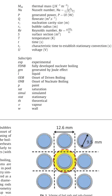
Although there were several studies about the transient boiling, especially in pool boiling, not all the physical mechanisms are understood. Moreover, except for Visentini et al.[12]study in pool boiling, none of the previous studies were made in a geometry sim-ilar to the one found in a nuclear core. The latter is idealized as a flow in an annular cross section with equivalent hydraulic diame-ter of the typical sub-channel defined between neighboring rods (in yellow1_{inFig. 1). To conduct experiments in a simple geometry} but similar to this sub-channel, an experimental set-up was designed by Visentini et al.[12]. To measure the wall temperature with a high temporal and spatial resolution, the infra-red thermog-raphy was used and so an optical access to the wall was needed. Therefore a half-annular cross section with the heated inner half cylinder has been preferred to the annular one.

The objective of this work is to understand and to model the incipience of the nucleate boiling in an upward semi-annular flow with an inner wall heated at different heating rates. In order to study the ONB in our experiment, the wall is heated by Joule effect with different power steps for short times to simulate transients, unlike the previously mentioned studies where the walls are usu-ally heated with exponential powers. This was done for different Reynolds numbers and sub-cooling in the continuity of the studies initiated by Visentini et al.[12].

2. Experimental set-up and measurements techniques

In this section, we introduce the main features of the facility. More details can be found in [12]. The test section has a semi-annular shape. The inner half cylinder consists of a 50

l

m thick stainless steel foil heated by Joule effect. Its diameter is 8.4 mm and its length 200 mm. The outer part consists of a 34 mm internal diameter glass half cylinder (Fig. 2). The semi-annular section is filled with a coolant 1-methoxyheptafluoropropane (C3F7OCH3), which will be referred as HFE7000 (3 M). This fluid has been cho-sen because of its low saturation temperature (35 "C at atmo-spheric pressure), its low latent heat of vaporisation (ten times smaller than the water one), and the smaller critical heat flux value compared to water. These characteristics have been chosen to

Fig. 1. Scheme of fuel rods and sub-channel.

1 _{For interpretation of color in Figs. 1 and 7, the reader is referred to the web}

version of this article. Nomenclature Greek symbols

a

thermal diffusivity,

a

¼ k

qCp(m

2_s!1₎ dt thermal boundary layer thickness (m)

k thermal conductivity (W m!1K!1) kc critical size (m)

l

dynamic viscosity (Pa s)

m

kinematic viscosity (m2_s!1₎ / heat flux (W m!2)

q

density (kg m!3₎

r

surface tension (N m!1₎

s

characteristic time (s) Latin symbols ! U mean velocity !_{U ¼ Q=S (m s}!1₎ Bi _{Biot number, Bi ¼}h ew kw

Cp specific heat capacity (J kg!1K!1)

Dh hydraulic diameter (m) E _{thermal effusivity E ¼ ffiffiffiffiffiffiffiffiffiffiffi}k

q

Cp p (J K!1_m!2_s!1/2₎ e thickness (m) G mass flux (kg m!2_s!1₎

h _{heat transfer coefficient, h ¼} /w Tw!Tl(W m

!2_K!1₎ hlv latent heat of vaporisation (J kg

!1₎ I current (A) Ja _{Jacob number Ja ¼}qlCp;lDT qvhlv L foil length (m) l foil width (m) Mth thermal mass (J K!1m!2) Nu _{Nusselt number, Nu ¼} /wDh kwðTw!TlÞ P _{generated power, P ¼ UI (W)} Q flowrate (m3_.s!1₎

rc nucleation cavity size (m)

re bubble radius (m) Re _{Reynolds number, Re ¼}qlUD! h ll S surface section (m2₎ T temperature (K) t time (s)

tc characteristic time to establish stationary convection (s)

U voltage (V) Subscripts

exp experimental

FDNB fully developed nucleate boiling gen generated by Joule effect l liquid

ODB Onset of Driven Boiling ONB Onset of Nucleate Boiling p paint sat saturation simul simulated stat stationary th theoretical

v

vapour w wall

perform highly transient boiling experiments with a lower power than required for water. The main physical properties of HFE7000 at saturation temperature and atmospheric pressure are given in theTable 1, where

q

; Cp; k and

m

are the density, heat capacity, thermal conductivity and kinematic viscosity, respec-tively. hlvis the latent heat of vaporisation and

r

the surface

ten-sion of the fluid. Physical properties of water at 155 bar are given in theTable 1for comparison.

The metal half-cylinder is glued to two lateral quartz glass plates (thickness: 3 mm, width: 42 mm, length: 200 mm). The plates, together with the foil, are placed in an aluminium cell. In this cell, a visualization box filled with HFE7000 is used to reduce optical distortions.

The experiments are carried out in flow boiling conditions by inserting the test cell in a two-phase flow loop consisting of a gear pump, a Coriolis flow meter, a pre-heater, a 1 m long channel upstream the test section to establish the flow and a condenser. The inlet temperature and pressure of the test section are mea-sured by a thermocouple and an absolute pressure transducer. The flow-rates investigated vary from 0.1 to 0.3 l s!1_{corresponding} to mass fluxes from 323 to 969 kg.m!2_s!1_{and corresponding to} Reynolds numbers from 14,000 to 60,000. The velocity profiles in the test section in single-phase flow have been measured by PIV in the mid-plane and characterized in the whole test section by numerical simulations by Baudin et al.[13]. The inlet fluid temper-ature is controlled by a chiller TERMOTEK P805, and the sub-cooling investigated vary from 5 to 20 K. So the sub-sub-cooling dimen-sionless Jakob number, defined as Jasub¼qlCpqlðv hTsatlv!TlÞ

, is between 8 and 33. This number is based on the liquid sub-cooling Tsat! Tl and represents the amount of energy required to heat up a mass of liquid from Tl to Tsat normalized by the energy required to vaporize the same mass of liquid. In our context, the larger the Jakob number, the higher the condensation rate in the bulk or the larger the delay for wall nucleation favourable conditions. The electrical power is provided by a power supply SORENSEN SGA. It covers the 0–40 V voltage range and the 0–250 A current range. The power supply is driven by an arbitrary generator to impose power steps of different powers and durations. The power supply can provide a current increase up to 45 A s!1_{. A voltmeter} and an ammeter measure the voltage U and current I to calculate the generated power in the metal foil P = UI.

Finally in a PWR, the refrigerant used is water. The thermohy-draulic conditions are P = 155 bars and T

#

[300–1500] "C with a cylinder fuel rod with an internal radius ri= 4.8 mm and external radius ro= 7 mm. The Reynolds number is equal to 400,000. In our model set-up, the fluid used is the HFE7000. The thermohy-draulic conditions are P = 1 bar and T

#

[20–300] "C with a semi-annulus section with an internal radius ri= 4.2 mm and external radius ro = 17 mm. The Reynolds number is between 0 and 60,000. There are differences between normalized numbers (Nus-selt or Reynolds number . . .) but the goal of our experiment was to be able to study the transient boiling with simplified conditions Fig. 2. Schema of the test section.

Table 1

Thermophysical properties of different materials.

Solid Foil properties at 20 "C (stainless steel AISI 304) qw(kg m!3) Cp;w(J kg!1K!1) kw(W m!1K!1)

7930 500 16:18

aw(m2s!1) Ew(J K!1m!2s!1/2) ew(lm)

4:08 % 10!6 8010 50

Solid Paint properties at 20 "C

qp(kg m!3) Cp;p(J kg!1K!1) kp(W m!1K!1)

1200 1480 0:13

ap(m2s!1) Ep(J K!1m!2s!1/2) ep(lm)

7:3 % 10!8 480 25 ! 30

Fluid HFE7000 properties at Tsat= 35 "C and at P = 1 bar

ql(kg m!3) Cp;l(J kg!1K!1) kl(W m!1K!1) 1376 1185 0:073 al(m2.s!1) ml(m2s!1) hlv(kJ kg!1) 4.5%10!8 _{2:8 % 10}!7 132 qv(kg m !3_{) r(N m}!1₎ 7:9 _{4:7 % 10}!3

Fluid Water properties at Tsat= 345 "C and at P = 155 bar

ql(kg m!3) Cp;l(J kg!1K!1) kl(W m!1K!1) 594 8950 0:46 al(m2s!1) ml(m2s!1) hlv(kJ kg !1₎ 8.65%10!8 _{1:15 % 10}!7 967 qv(kg m !3_{) r(N m}!1₎ 102 _{11:45 % 10}!3

and reach every boiling regimes with a limited required electrical power.

2.1. Wall temperature measurements

Measurements are performed with an infra-red camera looking at the foil from backward (seeFig. 2). A CEDIP JADE III camera with a sensitivity range between 3.5 and 5.1

l

m is used. It has a focal plane array detector cooled by a Stirling MCT. For this study, the acquisition frequency is 500 fps and the height of the metal foil investigated is about 7 cm in the z direction (Fig. 2). The integra-tion time is between 20 and 500

l

s for a spatial resolution of 240 % 320 px2_{. The infra-red camera is calibrated thanks to a} DCN 1000 N4 black body. The uncertainties on the measurement temperature of the black surface depend on the temperature range of calibration. For a low temperature range calibration (20–100 "C), the uncertainty is about &0.6 "C at 20 "C and &0.1 "C at 100 "C. For a high temperature range calibration (20–250 "C), the uncertainty is about &3 "C at 20 "C but only &0.3 "C at 250 "C. These uncertain-ties take into account the non uniformity of the black body temper-ature surface and the noise on the camera sensor. The tempertemper-ature and the heat flux measurements are made on the area between 5 and 15 cm from the bottom of the heated foil (' 3 ! 8Dh), each temperature measurement is averaged on 2 % 2 mm2_.

The thermal gradient across the foil thickness is expected to be negligible, since the Biot number Bi characterizing the thermal resistance of the foil by comparison to the thermal resistance of the flow is very small. For a high heat transfer coefficient, charac-teristic of transient boiling, h = 6000 W m!2_K!1_{, the Biot number is} equal to Biw¼ h ew=kw= 0.02, ew¼ 50

l

m being the foil thickness. The foil properties at ambient temperature are given inTable 1. Due to the small value of Biwthe foil temperature will be consid-ered constant in the thickness. Moreover, the diffusion time across the foil thickness

s

diff ;w¼ e2w=

a

w= 0.6 ms, is actually small enough to assume that there is no time lag between the thermal evolution of both sides of the metal foil. The thermal effusivity Ew character-izes the ability of a material to exchange thermal energy with its environment.

To obtain sufficiently precise temperature measurements, the backside of the metal foil is covered with a layer ('30

l

m thick-ness) of black paint with large emissivity (0.94). The black paint used is a Belton Spectral RAL 9005 MAT BLACK paint, which ther-mal properties were measured by the company NeoTIM (Albi,

France), and are given in Table 1. For a heat transfer coefficient of h = 6000 W m!2_K!1_{, the Biot number of the paint layer is} Bip' 1:2 (for a paint thickness of 30

l

m), which means that a small temperature gradient can exist between the surface of the paint (IR camera side) and the metal foil. The diffusion time across the paint thickness is about

s

diff ;p'0.01 s so some time lag can be expected. We do not notice a significant change in the measurement of the resistance of heated foil without and with paint, so we made the assumption that the paint is not electrically conductive. In a previous study[8], 2D transient heat conduction in the metal foil (without the black paint layer) performed with COMSOL Multi-physics have shown that the conduction in the lateral direction remains very small. Thus a 1D transient conduction model inside the metal foil and the paint is used to characterize the effect of the paint on the thermal measurement (temperature gradient and time delay).Fig. 3shows the result of this model for a paint thickness of 25

l

m and a steady heat transfer coefficient of 1000 W m!2_K!1_{. As one can see the temperature gradient in the} paint is small and becomes quickly negligible: except for strong temperature variations ((dT/dt)/(d2_T/dt2

(

s

diff), the temperature evolution on the paint side corresponds to the evolution on the liq-uid side with a lag time of about 0.05 s.

This model also shows that the heat flux from the wall to the fluid /wcan be calculated using the simple thermal balance:

/w¼ /gen!

q

wCp;wewþ

q

pCp;pep

# $dT_w

dt ð1Þ

wheredTw

dt is the wall temperature variation. The natural convection and radiation heat transfers between the air and the paint are neglected since the corresponding heat fluxes (< 400 W m!2 _for both) are small in comparison to the generated power (> 10 kW m!2_).

A National Instruments box CompactRIO9035 is used to acquire the thermocouples (flow temperature control), pressure, flow and power measurements. The uncertainties of the electronic devices (ammeter, National Instrument box) are very low and of the order of magnitude of 0.1% (Visentini[8]). The power generated by Joule effect per surface unit /_genis equal to U:I/L:l where L the length of the foil and l its width. The main uncertainty comes from the length of the part where the voltage is measured (about &0.2 cm on 8.5 cm i.e. about 2%). Thus the total uncertainty on /gen is 2.5%, which is also the uncertainty on the heat flux in steady state. The heat transfer from the wall to the fluid is calculated with

Eq.(1). Assuming that

q

wCp;wewþ

q

pCp;pep¼ 242 J m!2has a low uncertainty (the thermal properties of the stainless steel and paint are known and in our range of temperature, the thermal inertia variation is 10% maximum). The absolute uncertainty on the heat flux is:

D

/w ð Þ2¼ _@/@/w gen " #2

D

/2genþ @/w @ep ' (2

D

e2p þ _{@ dT=dt}@/w ð Þ ' (2

D

_ðdT=dt_Þ2 _ð2Þ

The generated heat flux varies from 40 to 400 kW m!2_{, and the} temperature time derivative at the onset of nucleate boiling varies from 10 to 500 K s!1_{. So the wall heat flux uncertainty can reach} 6.5% of its value.

2.2. Transient convection

Baudin et al. [13]studied the turbulent flow and convection heat transfer in a semi-annulus through experiments and numeri-cal simulations. The numerinumeri-cal simulations were made with the software StarCCM + including the resolution of RANS equations using a k-

#

model and resolution of the equation of the energy in the fluid and in the solid composed of the foil only. They observed that the wall temperature evolution is self-similar when scaled by the steady wall temperature and that transient regime is charac-terized by a time scale tc which depends only on the Reynolds number (through the Nusselt number).

These simulations were performed without a paint layer, and only the metal foil thermal mass characterizes the time scale evo-lution while, in their experiments, the metal foil was painted with a layer of thickness around 100

l

m. Thus, experimentally, the wall thermal mass was high (' 178 J m!2_K!1_{) and induced} uncertain-ties on the heat transfer coefficient at the beginning of the heating. In the present study the paint thickness is about 30

l

m, the wall thermal mass is thus low (' 44 J m!2_K!1_{) and the uncertainty on} the heat transfer coefficient during the first times is low.

The experimental wall temperature and the dimensionless heat transfer coefficient evolutions during a power step are plotted respectively on the left hand side and right hand side inFig. 4. This measurement is an average temperature at the top of the foil (height = 0–3.5 cm) in the central part of the metal foil to avoid entrance phenomenon.

At the beginning of the heating, the thermal boundary layer is not established yet, thus the heat transfer coefficient is higher than in steady state. For both the heat transfer coefficient evolution and

the wall temperature evolution, the characteristic time to reach steady state decreases when the Reynolds number increases. How-ever, while the wall temperature is steady after about 1–5 s, the heat transfer coefficient is steady after about 0.2–0.75 s.

The advection time defined with the length of the heating sur-face and the average velocity is:

s

adv¼

L

U¼ 0:15—0:5 s ð3Þ

with the average velocity U ¼ 0:1—0:7 m s!1_{for Q ¼ 0:05—0:4 l s}!1_. The turbulent mixing time can be estimated from an estimate of the typical eddies length Leddiesby:

s

mix¼ Leddies U0 ¼

j

Dh 0:05U¼ 8:2Dh U ¼ 0:11 ! 1:3 s ð4Þ

with the constant of Von Karman

j

= 0.41.

The advection characteristic time

s

adv, taken at the center of the

flow, is lower than the forced convection times measured. Due to inlet flow, the flowing liquid temperature is kept constant and equal to the sub-cooling temperature imposed in the hydraulic loop.

The characteristic times of mixture

s

mixare in good agreement with the times obtained experimentally. The vortices in the mix-ture contribute to the development of the thermal boundary layer and are therefore characteristic of the forced convection regime establishment. In this case, the heating rates imposed during this regime are low and the heat transfer is not due to unsteady con-duction but rather to the forced convection since the eddies control this regime. The heat transfer coefficient characteristic time is thus directly related to a turbulent time scale.

Baudin et al.[13]pointed out a linear decrease of dTw/dt, thus, a quasi-steady evolution of the wall temperature can be assumed (i.e. assuming h ¼ hstat). This is indeed sufficient as long as we do not focus on the very first times of the transient. The heat transfer coefficient during a test achieved quickly its steady state since the paint thickness is low so:

Twð Þ ! Tt 0 Tw;stat! T0¼ 1 ! e !t=sth _ð5Þ

s

th¼ Mth hstat ð6Þ

hstat is the steady convection heat transfer coefficient and Mth¼

q

Cpe is the thermal mass of the wall. Only the heated foil is considered in the simulations, the thermal mass is Mth;w¼

q

w Cp;wew. For the experiments, the paint layer is included: Mth;wþp¼

q

wCp;wewþ

q

pCp;pep. The good agreement between the

time scales calculated from the simulations/experiments with Eq.

(6)is shown onFig. 5. Although the steady state heat transfer coef-ficient in[13]was obtained for an area 13 cm away from the bot-tom of the foil, these values decrease or increase of maximum 2% on the studied area of this article. Therefore this value is kept to model the temperature evolution on this whole surface.

The thickness of the thermal boundary layer including the vis-cous and buffer layers has been obtained from the results of numerical simulations Baudin et al. [13] and is defined as

s

sim. From the evolution of the wall temperature,

s

simwas deduced from Eq.(5).

3. Analysis of the onset of boiling

In all this section, we analyse in details the phenomena occur-ring duoccur-ring the transition from single-phase to nucleate boiling regime following a step in power starting from zero. The analysis focuses first on a single test condition, and all the time and/or space evolution refer to these test conditions:

Then the analysis is generalized to a set of test conditions that have been considered, varying the power level as well as the flow conditions. Flow rate corresponds to different colors. red: 0.1 l s!1_, blue: 0.2 l s!1_{, green: 0.3 l s}!1_{. Liquid bulk temperature correspond} to different shapes. The sub-cooling of the inlet liquid flow

D_{T ¼ T}sat! Tl (that is also the initial wall temperature sub-cooling) is , :D_{T ¼ 13}-_{C; ! :DT ¼ 15}-_{C and } :DT ¼ 17}-_C. Finally, the generated heat flux, Ugen is between 40,000 and 80,000 W m!2_.

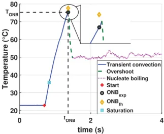
3.1. A generic time evolution for local wall temperature

All over the test section, and for any test condition that leads to the onset of boiling, the time evolution of wall temperature is rather similar. Such a typical process is illustrated on the graph ofFig. 6. As the power is set to its constant non-zero value (red symbol around t ¼ 1 s on the graph), the wall temperature first increases from its initial value, that equals to the sub-cooled liquid temperature within the test section. It follows an exponential relaxation like for the purely single-phase tests described in Sec-tion2.2: the blue part of the curve. It goes beyond the saturation temperature value (blue square) without any noticeable deviation until it reaches a maximum (the black dot, after the ONB) whose value corresponds to an overheat of approximately 40-_{C with} respect to saturation temperature. Then a rather sharp decrease

(the green dashed lines denoted overshoot on the graph) occurs over a fraction of a second. Temperature then reaches a quasi-constant level (the purple part of the curve around 50-_{C in this} case) that is still over the saturation value and will be considered as the steady local temperature for such a test. Small perturbations of few degrees around a constant value can be seen on the curve. The rather low wall superheat corresponds to typical nucleate boil-ing regime.

From this analysis of the wall temperature, one clearly identi-fies two different stages in the transition from the initial to the final steady states: the increase, that is very similar to the transient convection, followed by a sharp decrease. The overshoot of temper-ature (i.e. the difference between the local transient maximal tem-perature and the final steady value) is relatively large, around 25-_{C, even larger than the wall superheat at the steady state} (around 15-_C).

3.2. Sketch of the two-phase flow pattern at the onset of boiling OnFig. 7, several snapshots of the high speed camera are pro-vided for a single test and at different times. The heated wall cor-responds to the thick black area on the right hand side of each picture. The high-speed camera is placed perpendicularly to the infra red camera and takes pictures in the (x,z) as indicated in

Fig. 2) and the high-speed camera visualizations are made by ombroscopy. The small hyphen indicates a 1 mm long scale. During the test, the metal foil is measured on a field of 20 % 120 pix2 where 1 pixel is equal to 0.047 cm. The high-speed camera visual-ization is 384 % 1024 pix2_{where 1 pixel is equal to 0.008 cm. So} the High-speed Camera space resolution is sufficiently high with respect to the typical bubble size (/10 pixels for the diameter of a bubble during the nucleate boiling). It’s not the case for the infra-red camera where it’s not possible to see the bubble feet clearly. Finally, due to technical performance the High speed cam-era and infra-red camcam-era sampling frequencies are 500 Hz which is not sufficient to see the first steps of the bubble nucleation (see

Fig. 7).

The left hand side photo corresponds to the time, denoted tONB at which the first deviation from the initial state has been catched by the ad hoc algorithm of image treatment. Only a zoom on the surrounded area could provide a clear evidence of an event for a direct visual observation. It is seen that 6 ms after (second picture), a vapor bubble of less than 1 mm thickness and a few mm long covers a part of the wall. It then grows or expands rapidly over Fig. 5. Wall temperature characteristic time in forced convection, compared to

theory, for experiments (M_th;wþp¼qwCp;wewþqpCp;pep) and simulations

(Mth;w¼qwCp;wew) versus the Reynolds number.

Fig. 6. Temporal evolution of wall temperature in the close vicinity of the first nucleation event.

the tens of ms after its apparition, mainly in the axial direction. At its top end, it reaches quasi a 1 cm thickness whereas the vapour layer just below is composed of relatively smaller quasi spherical bubbles (like on the (e) picture). A few tenths of second after tONB, the wall is covered by a population of tiny bubbles (1 mm). This corresponds to times for which the wall temperature is stabi-lized. This flow pattern will be recovered during the next seconds also and corresponds thus to the steady configuration. Let us also remark that almost no bubble exists far from the wall, that is typ-ical from such convective sub-cooled boiling case.

3.3. Localized first nucleation event

The wall temperature evolution reported inFig. 6corresponds to the location where the first temperature maxima is reached. This location coincides with the area outlined in red on picture

a

ð Þ ofFig. 7which correspond to the first bubble. It can appear any-where around the semi-circular heated surface. In this case, the first bubble is nucleated on the front part of the foil (marked with a red zone). It then propagates around and along the heated foil. The time tONB, deduced from the high-speed camera, corresponds to the black point on the temperature evolution: it is very close to the time for maximal temperature. The apparition of the first vapor bubble coincides in space and time with the first tempera-ture decrease over the test section.

This correspondence is common to all the 50 tests where those events occur in the scope of both cameras. The value TONBof the temperature at the location of the first event and at the time tONB has been collected for several test sections and flow conditions. The values are always close to the local maximum at this location. They are reported on Fig. 8 and are slightly in the range

60-_{C : 80}-_C

½ 1. This value is compared to the theoretical tempera-ture for transient convection at the same time tONB as given by the Eq.(5)validated on our study of this regime. OnFig. 6, it cor-responds to the yellow diamond that slightly over-predicts the maximum value. For the set of tests considered, it is shown in

Fig. 8that this theoretical prediction is in a rather good agreement with experimental measurements, with a small tendency to over-predict the measured temperature with the model. Therefore, at first order, the temporal evolution of wall temperature at the loca-tion where nuclealoca-tion will first take place is the one of transient convection until this time. No sign of any precursor event seems to be deducted from our thermal measurements.

The measurement of Tonb;exp is made by the infra-red camera with an error of approximately &0.1-_{C. The error bar corresponds} to the symbol size.

3.4. Temperature at nucleation event and cavity size

The theoretical equilibrium superheat of a radius vapour bubble recan be calculated from Laplace and Clapeyron equations:

D

Teqð Þ ¼ Tre eqð Þ ! Tre sat¼

2

r

Tsat

q

vhlvre

ð7Þ

For a bubble in a cavity of size rc, Hsu [14] advises to take re¼54rc. From the experimental values of DTONB and Eq. (7), the cavity sizes on the metal foil that would correspond to the observed onset are about 0.11–0.15

l

m. Microscope and AFM visu-alisations showed that the heated foils have lamination grooves 1– 10

l

m large and 0.1–0.2

l

m depth, with surface cavities from 50 nm to 0.2

l

m. The contact angle of the HFE7000 on the metal Fig. 7. Visualizations of the onset of boiling. The first vapour bubble (ONB) (a) grows in a large vapour layer along the wall (b–c), then breaks and disappears (d) leading to boiling driven regime (ODB) (e) to finally reach the Fully Developed Nucleate Boiling (FDNB) (f).

foil has been measured of about 13" with a tensiometer DSA100. Big cavities, that would require low wall superheat to be nucle-ation sites are easily flooded, that inhibits nuclenucle-ation. Therefore, nucleation is more likely to occur for high superheat temperatures are expected, corresponding to small cavities with rc¼ 0:11—0:15

l

m.

Hsu’s model takes into account the growth of the thermal boundary layer in the liquid: the nucleation occurs only when the liquid at the top of the bubble (at rb¼ 2rc) is at the equilibrium temperature calculated with Eq.(7). Berthoud et al.[15]and Su et al. [11]suggested and used this model to calculate the onset of nucleate boiling for transient heatings. Assuming a linear profile through the thermal boundary layer, the first vapour bubble super-heat can be written:

D

TONB¼

D

Teqð Þ þrc

2rc

dt;tONB

TONB! Tb

ð Þ ð8Þ

This equation shows that the wall temperature at nucleation is the sum of the theoretical equilibrium temperature in the homoge-neous case plus the thermal gradient across the bubble of size 2rc. This second term introduces an impact of the wall heating rate on

the nucleation temperature. It also depends on the cavity (and therefore on the bubble) size: the smaller the cavity size, the closer the nucleation temperature to the equilibrium one.

According to the Section2.2, the evolution of the temperature and the thermal boundary layer thickness are self-similar during forced convection. Therefore, Eq.(8)can be written:

D

TONB¼

D

Teqð Þ þrc 2rc dt;stat Tstat! Tb ð Þ ð9Þ '

D

Teqð Þ þ 2rrc c /gen kl ð10Þ

In this last equation, the steady thermal boundary layer thick-ness is approximated by dt;stat' kl=hstat. Eq.(10)is plotted on the left hand side graph ofFig. 9with a dashed line for different rc. The second term of Eq.(10)varies from 0.1 to 0.2 K in the experi-ments: the onset of boiling superheat appears to be nearly constant for a given cavity size and equal to the equilibrium superheat.

Su et al.[11]study transient ONB with an exponential heating with a characteristic time

s

and their surface has small cavity sizes in comparison to the thermal boundary layer thickness. They show thatDTONBcan be well estimated with:

D

TONB¼

D

Teqð Þ þrc rc dt

D

Teqð Þ þrc

D

Tsub ) * ð11Þ

with dt¼ ffiffiffiffiffiffiffipal

s

for pool boiling (conduction heat transfer in the liq-uid) and dt¼ kl=hstatfor dominant convective boiling. Eqs.(11) and (8)are very similar; however, in Su et al.’s study, the convective characteristic time is very small (maximum 110 ms) and they can consider an established thermal boundary layer when the nucle-ation begins.

Using Eq.(5)from2.2and Eq.(10), the first vapour bubble time can be calculated by:

tONB' ! Mth hstat ln 1 !

D

Teqþ

D

Tsub ) _*h stat /gen ! 2rchstat kl ! ð12Þ

The first contribution in the logarithm corresponds to the time to increase the wall temperature to Teqand the second contribution corresponds to the time to have the temperature Teqat the top of the bubble, which is again negligible. Eq. (12) is plotted with a dashed line in the right hand side graph of theFig. 9and shows a rather good agreement with the experimental points. These experiments have been performed with three different test sec-tions which could explain the dispersion of the results due to small difference in the surface state. The points above the dashed curves might correspond to smaller cavities.

Fig. 8. Experimental value of the temperature at the first nucleation event TONB;exp

compared to the theoretical temperature for transient convection (Eq.(5)) at the same time TONB;thfor different test conditions. Flow rate corresponds to different

colors. red: 0.1 l.s!1_{, blue: 0.2 l s}!1_{, green: 0.3 l s}!1_{. Sub-cooling corresponds to}

different forms, , : DT ¼ 13-_{C; ! : DT ¼ 15}-_{C and } : DT ¼ 17}-_{C. (For}

interpreta-tion of the references to colour in this figure legend, the reader is referred to the web version of this article.)

Fig. 9. Temperature and time of nucleation for different test conditions. Flow rate corresponds to different colors. red: 0.1 l s!1_{, blue: 0.2 l s}!1_{, green: 0.3 l s}!1_{. Sub-cooling}

corresponds to different forms, , : DT ¼ 13-_{C; ! : DT ¼ 15}-_{C and } : DT ¼ 17}-_{C. (For interpretation of the references to colour in this figure legend, the reader is referred to}

The superheat at the time of the nucleation event

DTONB¼ TONB! Tsat has been plotted against the level of power intensity of the considered test /gen onFig. 9. This wall superheat does not change much, neither with the heat flux, neither with the flow-rate, nor with the sub-cooling, and remains around 40 "C. 3.5. Delayed onset of boiling over the test section

In Fig. 10, the temporal evolution at different locations along the test section has been plotted on the same graph. They are indexed by the Z variable that measures the vertical distance from the location of the first nucleation event Z4;ONB¼ 0 cm that also cor-responds to the first decrease.

It can be seen that the time for the local maximum is all the more delayed with respect to tONBthat this distance is large. The delay is approximately 0:5 s for a 2 cm distance. This time scale is relatively of the same order of magnitude than the time scale for local relaxation from the maximum temperature to the steady value. We observe that such a delay is very reduced in the radial direction over the wall, in particular as soon as locations suffi-ciently far from the nucleation event are considered. Let us remark also that the temperature continues to notably increase after tONB in the other locations than at the location of the event. Moreover, it can be seen a specific trend at the very last times of increase: the temperature increase rate seems to increase rather than decrease (the curve is rather convex than concave). After the decrease, all the temperatures converge toward approximately the same value around 50-_{C. The overshoot of temperature} depends therefore of the location considered. As a consequence, during the onset of the nucleate boiling regime, the deviation of temperature around a space average value (like the black curve on the graph) is relatively large. This leads to a difficulty in the interpretation of such averaged value in terms of nucleation mech-anisms. The maximal value of the mean temperature is rather low with respect to local values and should be compared with caution with any model for nucleation. The typical relaxation time of the average temperature toward the steady value is clearly a combina-tion of the local relaxacombina-tion time that looks at first order very similar at different locations with the delayed decrease that looks like a front propagation.

3.6. Cooling at the onset of nucleate boiling

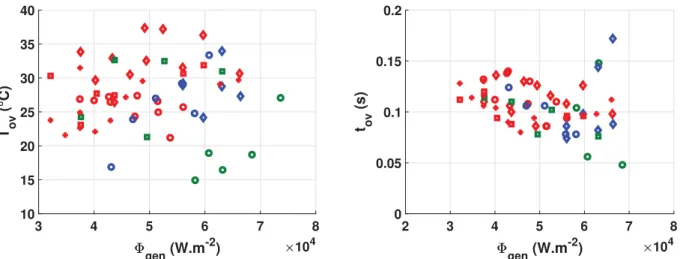
Let us focus on the local temperature decrease from the maxi-mum temperature, say Tmax toward the steady nucleate boiling

temperature, say TNB. The difference between those two values is then referred to a transient overshoot TOV¼ Tmax! TNB. The tran-sient cooling is analysed locally for the location of the first nucle-ation event. The overshoot is therefore the minimum one with comparison to other locations for the same test. It has been plotted for different test conditions on the left hand side graph ofFig. 11. The overshoot order of magnitude is approximately tens of degrees but no clear tendency can be deduced and the dispersion is large. The time tOVbetween the maximal temperature and the first time it reaches the steady value TNBhas been plotted on the right hand side ofFig. 11. The value is typically around 0:1 s with a rather small dispersion and no clear tendency with respect to the test conditions: liquid flow rate and sub-cooling.

The left hand side graph ofFig. 12is a focus on the decrease phase of wall temperature at the nucleation site where the temper-ature time evolution has been reduced as Tþ_{¼ T ! T}

NB

ð Þ= Tð OV! TNBÞ. The experimental measurement is clearly well fitted by an exponential law Tþ_{¼ exp !t=}

_s

OV ð Þ. For each test condition considered the value of the best fit for the parameter

s

OV has been reported on the right hand side graph of Fig. 12. The value is typically around 0:03 s with a rather low dis-persion and no clear tendency with respect to the different test parameters.

It indicates that the cooling process during the transient estab-lishment of nucleate boiling heat transfer at the location of the first nucleation event is very efficient (with a cooling rate of several hundreds of K s!1_{). This cooling process seems insensitive to the} flow and power conditions.

3.7. A vapor front propagation

For each pixel of the high-speed camera images, i.e. for each axial location along the wall, the vapor layer thickness Db½ 1 ism the instantaneous lateral length corresponding to the number of pixels identified as being in vapor phase. This quantity can be asso-ciated with the size of the bubbles that can be seen on the pictures. The time and space evolution of the quantity Dbis reported on the picture ofFig. 14a.

An algorithm allows to track the time at which a vapor layer appears. For this test, this first event is located at Z ¼ 3:07 cm as represented by the grey circle. The white solid line joins the times of vapor apparition at each axial location z. It corresponds there-fore to the boundary of non-zero vapor layer thickness above the wall. The vapor propagation is linear meaning the vapor layer pro-gression has a constant axial velocity from its starting point at the first nucleation event, both downstream and upstream in this case. The white-dashed line corresponds to the maximum bubble height.

From the white lines slopes, the propagation speed of the vapor front along the vertical direction has been deduced for several test conditions. As shown on theFig. 13, the velocity lies in the range

50

½ cm s!1_{–100 cm s}!1_{1 and is larger in the downstream/upward} direction (positive velocity) than in the upstream/downward direc-tion probably because of both the liquid flow and the buoyancy that should assist the vapour propagation in the upward direction. Let us remark, that in some cases (more especially for the lar-gest flow rates), there is no data for upstream propagation of the vapor front, since it does not propagate upstream from the nucle-ation point identified. The area can be kept without boiling for a while. Possibly, another nucleation event occurs downward and nucleate boiling regime propagates toward the region.

During its axial progression downstream (upward), the vapor front has an increasing thickness until an approximately 7 mm extent (dark red zone for z < 1 cm and t ’ 0:1 s). The time when Dbfirst decreases corresponds to the tail of the vapor pocket. Its Fig. 10. Wall temperature at different locations along the test section.

trajectory (location of local Db maximum) has been determined thanks to an algorithm and is plotted as the white dashed line

(the rightmost line) onFig. 14.a. This line is approximately parallel with the apparition of the vapor (white solid line) with a delay of approximately 0:02 s.

Other relatively large vapor pockets growing along the wall can be detected afterwards (see the light green area parallel to the white line). They can be seen until approximately 0:15 s and their size is approximately 3 mm. It still corresponds to the transient period of nucleate boiling regime establishment. They could be associated with other nucleation events downstream that could initiate other large vapor pockets, but this is not evident to be con-clusive on this behaviour.

After t ’ 0:15 s, Dbdecreases to approximately 1 mm, that cor-responds to the size of the tiny bubbles in the steady sub-cooled nucleate boiling process.

3.8. Thermal analysis of the transition toward nucleate boiling The wall temperature as a function of time and space is plotted in theFig. 14b.

Temperature is relatively homogeneous in space during the first 0:05 s and after 0:15 s where it reaches a notably steady lower value. Let us focus on the transition zone between these two regimes. The lines deduced from the vapor front thickness analysis have been reproduced. It can be clearly seen that the wall Fig. 11. Overshoot: temperature difference and typical time for temperature decrease. Flow rate corresponds to different colors. red: 0.1 l s!1_{, blue: 0.2 l s}!1_{, green: 0.3 l s}!1_.

Sub-cooling corresponds to different forms, , : DT ¼ 13-_{C; ! : DT ¼ 15}-_{C and } : DT ¼ 17}-_{C. (For interpretation of the references to colour in this figure legend, the reader is}

referred to the web version of this article.)

Fig. 12. Exponential model for the cooling after the overshoot and determination of an overshoot characteristic time.

Fig. 13. Axial propagation velocity of the vapor front. Flow rate corresponds to different colors. red: 0.1 l s!1_{, blue: 0.2 l s}!1_{, green: 0.3 l s}!1_{. Sub-cooling}

corre-sponds to different forms, , : DT ¼ 13-_{C; ! : DT ¼ 15}-_{C and } : DT ¼ 17}-_{C. (For}

interpretation of the references to color in this figure legend, the reader is referred to the web version of this article.)

temperature continues its increase at the time (white lines) when the vapor front covers a specific location. The location of the max-imum of temperature seems to be more correlated with the white dashed line that corresponds to the tail of the first vapor pocket.

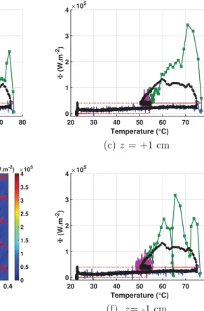
The wall to fluid heat flux, as deduced from Eq.(1), is plotted for the same case on the right hand side ofFig. 14c. The lines deduced from the vapor front thickness analysis have also been reproduced. The first convection phase corresponds to rather low values for the heat flux. The last steady phase corresponds to the equilibrium between the generated heat flux /genand the wall to fluid heat flux /w. The largest heat flux values are clearly associated with the white dashed line and could reach up to 4 % 105_{W m}!2 _values. This is fully consistent with the evolution of wall temperature (from which it is partly deduced). It is worth noting that those local heat flux values are very large in comparison with the order of magnitude of the critical heat flux that is close to 105_{W m}!2_in similar conditions (from our own experiments).

Fig. 16a represents the logarithm of the ratio /w=/gen of the same test. Once again, the black lines deduced from the analysis of the vapor front thickness analysis have been reproduced. It is

very close to 0 (i.e. /w’ /gen) as soon as the steady nucleate boil-ing regime is reached. Durboil-ing the transient convection stage, it indicates that the heat flux is approximately one order of magni-tude less than the power intensity. The boundary of this regime is a short period represented by a rather thin orange line near the black dashed line. The heat flux is for a small fraction of time of the magnitude or larger than the power intensity. Despite this very evanescent step, the transition between those regimes is clearly made of two successive steps. The first one occurs when the first big vapor pocket covers the wall, i.e. between the black solid and the black dashed lines. It corresponds to a quasi-null heat flux toward the fluid (until around 1000 times less than the power dissipated). This corresponds clearly to the inflexion of the wall temperature just before the decrease that has been identified on the temporal local evolution of the wall temperature in Section3.5. It is followed by a very rapid increase of the wall to fluid heat flux with maximal values more than 10 times the power dissipated. The transient heat flux during this transition toward nucleate boiling regime is therefore a very efficient heat transfer.

Fig. 14. Vapor layer thickness, temperature and heat flux along the heated wall as function of time and axial location along the vertical (z ¼ 0 being the top of the picture and the axis being oriented downward).

A possible interpretation of this behaviour is therefore as fol-lows. Below the big vapor pocket that covers the wall following a first nucleation event, the heat flux is hindered. Due to the very low values of the wall to fluid heat flux, a transient dry-out of the wall can not be excluded. But this could also been explained by the fact that the vapor pocket insulated the wall from the rest of the flow and thereby of the efficiency of the coolant flow. When the pocket leaves the wall, the wall to fluid heat flux is suddenly very high: that could correspond to either the rewetting of the wall and intense vaporisation, or by the appearance of small bubbles in the tail of the large vapour bubble.

3.9. Local boiling curves

OnFig. 15, the local wall to fluid heat flux /was a function of the local wall temperature has been plotted at different axial eleva-tions. The transient evolution of /gen has also been represented by the red curve. Those elevations correspond to an horizontal line on the flux map. The fourth one corresponds to the elevation at which the first nucleation event occurs. Arrows on this curve indi-cate the time direction. Each curve, that can be associated to a more standard boiling curve, has been divided in three phases: in blue, the transient convection where the heat flux is always lower than the generated heat flux /gen, in dark green, the transition toward nucleate boiling regime and in purple the steady nucleate boiling regime where the mean heat flux equals /gen.

At the very end of the transient convection phase (i.e. in the blue part close to the maximal temperature), it can be seen on the top elevations that the heat flux tends to zero before increasing stee-ply. Then, the transition toward nucleate boiling regime occurs and the local heat flux reaches high values (approximately 3 105_{W m}!2_{) almost all the time for temperature decrease. The} evolution is rather similar between all locations. In some cases,

the heat flux can temporarily reach zero values during the transi-tion. It is associated to the trajectory of large vapor pockets (possi-bly other nucleation events) flowing from upstream and that could disturb the effective cooling process, eventually inducing local dry-out of the wall.

The mean boiling curve (the black line in the figure) has a reduced amplitude during the Overshoot and can not transcribe a local flux drops near the ONB. The classic approach of representing the boiling curve with a space averaged heat flux can not follow all the process during the onset of boiling that are mostly local and there is a lack of information with this representation. An addi-tional approach is now provided to study this transition toward the FDNB.

3.10. Impact of test parameters on the behaviour

For a same sub-cooling and for 3 different flow rate values, the level of power has been varied as illustrated by the reduced wall to fluid heat flux space and time variation onFig. 16. It shows that the behaviour is very similar for the different test conditions. The degradation of the wall to fluid heat flux (blue part) before the transition toward nucleate boiling is not seen in some high flow rate and relatively low power cases (d,g,h). In those latter cases, it can be seen on the high speed camera images, that the vapor pocket incoming from the nucleation site is not as large as in the other cases. This could be interpreted by the lack of any dry-out and therefore no heat transfer degradation. In some cases, it is seen that the wall upstream a nucleation site can be heated up during a relatively long time until another nucleation event leads to its cool-ing (like in the bottom part (z P 4 cm) of cases d or f). In those cases, several successive events of heat transfer degradation and front propagation can be identified. From a more general point of view, the onset of nucleate boiling is all the more delayed than

the flow rate is high. In some cases (g on the figure) the nucleation event occurs below (upstream) the frame of the IR camera. 4. Conclusions

An experimental study of the onset of convective nucleate boil-ing in transient conditions was performed in a geometry similar to a nuclear fuel rod surrounded by coolant. The flow Reynolds num-bers studied varied from 14,000 to 52,000 and the sub-cooling from 5 to 20 K. The transient heating was achieved imposing heat flux steps from 20 to 500 kW m!2_{, corresponding to heating rates} from 10 to 500 K s!1_{. Infra-red thermal measurements and} high-speed camera visualizations have been synchronized in space and time and original algorithms of image processing have been developed. It brings more knowledge on the detailed processes along the wall during the onset of nucleate boiling. Models for the transient mechanisms have been proposed that will help better understanding of the phenomena occurring during a reactivity ini-tiated accident in a pressurized water reactors.

The main findings of the study are:

4 The evolution of the wall temperature and the evolution of the thermal boundary layer thickness are self-similar during the forced convection regime. Thus, the characteristic time to estab-lish the wall temperature and the thermal boundary layer thick-ness is equal to the thermal mass of the wall over the steady convective heat transfer coefficient. It is important to take into account the thermal mass of the paint used to perform the infra-red thermal measurements. From the comparison between different characteristic time, we conclude that a quasi-steady model can predict well the temperature evolution during this regime.

4 For the process of boiling onset, it has been shown that it is mostly driven by localized nucleation events followed by prop-agation mainly in the flow direction. Therefore space averaged analysis of the process is not well suited and leads to artificial smoothing of the local time evolutions (in temperature or in heat flux).

Fig. 16. Reduced wall to fluid heat flux for different flow conditions; All cases are with DT ¼ 13-_{C. Flow rate is 0.1 l s}!1_{for the first line (cases (a–c)), 0.2 l s}!1_{for cases d–f and}

4 The very localized first nucleation event is well modelled by Hsu’s theory. While the flow-rate and sub-cooling did not change the results significantly, the nucleation site size pre-dicted by the theory is consistent with the size of cavities along the wall. The wall superheat and the time for the nucleation event are well predicted by the combination of the Hsu’s theory and the model proposed for transient convective heat transfer before nucleation.

4 The first vapour bubble at this nucleation site rapidly grows as a vapor pocket that spreads over the wall mainly in the flow direction. This insulates partially the heated wall: except at the first nucleation site, a first sharp decrease of heat flux toward near zero values coincides with the presence of the vapor pocket over the wall. The wall temperature thus increases until the vapour layer is too big and breaks up. Then, the nucle-ate boiling regime is activnucle-ated that leads to a rapid wall temper-ature decrease. The corresponding local heat flux can be very high, even larger than the critical heat flux and uncorrelated from the power level.

4 The vapor pocket grows when it propagates until approximately 7 mm thickness. Its propagation speed of the vapor pocket along the wall has been estimated and is larger in the flow direction since it is then driven both by gravity and drag from the flow. For the largest flow-rates, no upstream propaga-tion has been observed and on the corresponding downward parts of the wall nucleate boiling is triggered by other nucle-ation events.

4 The fine spatio-temporal analysis of both heat transfer and two-phase flow structure has evidenced the localized mecha-nisms beneath the triggering of nucleate boiling in such con-vective, turbulent, and sub-cooled flow with a rapid heating of a vertical wall. No homogeneous nucleation over the wall has been observed but rather a propagation from isolated nucleation sites. On one hand, space and/or time averaged analysis of such process could not reveal such features. On the other hand, localized measurements by thermocouples are insufficient to cover the relatively spatially inhomogeneous process over the wall.

4 Therefore, this study will allow a better interpretation of past experimental results, first from the studies of transient boiling over wires, plates or ribbons, but also more particularly, in the context of nuclear safety studies, from RIA dedicated tests of power pulse heating of fuel rods.

Conflict of interest None.

Acknowledgements

This work is funded by Institut de Radioprotection et de Sûreté Nucléaire (IRSN) and Électricité de France (EDF) in the frame of their collaborative research programs. The authors would like to acknowledge the technical staff of IMFT, especially Laurent Mouneix and Grégory Ehses, for helping with the experimental set-up. Frédéric Bergame is greatly thanked for his support in the implementation of heating control programs, also Sébastien Cazin for his support in the infrared measurements and the flow visualizations.

Appendix A. Supplementary material

Supplementary data associated with this article can be found, in the online version, athttps://doi.org/10.1016/j.ijheatmasstransfer. 2019.04.069.

References

[1]M.W. Rosenthal, An experimental study of transient boiling, Nucl. Sci. Eng. 2 (5) (1957) 640–656.

[2]A. Sakurai, M. Shiotsu, Transient pool boiling heat transfer-part 1: incipient boiling superheat, J. Heat Transf. 99 (4) (1977) 547–553.

[3]A. Sakurai, M. Shiotsu, Transient pool boiling heat transfer-part 2: boiling heat transfer and burnout, J. Heat Transf. 99 (4) (1977) 554–560.

[4]A. Sakurai, M. Shiotsu, K. Hata, K. Fukuda, Photographic study on transitions from non-boiling and nucleate boiling regime to film boiling due to increasing heat inputs in liquid nitrogen and water, Nucl. Eng. Des. 200 (1) (2000) 39–54. [5]H. Auracher, W. Marquardt, Heat transfer characteristics and mechanisms along entire boiling curves under steady-state and transient conditions, Int. J. Heat Fluid Flow 25 (2) (2004) 223–242.

[6]J. Jackson, L. Zhu, K. Derewnicki, W. Hall, Studies of nucleation and heat transfer during fast boiling transients in water with application to molten fuel-coolant interactions, Nucl. Energy 27 (1) (1988) 21–29.

[7]G.-Y. Su, M. Bucci, T. McKrell, J. Buongiorno, Transient boiling of water under exponentially escalating heat inputs. Part I: pool boiling, Int. J. Heat Mass Transf. 96 (2016) 667–684.

[8] R. Visentini, Étude expérimentale des transferts thermiques en ébullition transitoire, Ph.D. thesis, Thèse Université de Toulouse (INPT),<http://ethesis. inp-toulouse.fr/archive/00002037/>, 2012.

[9]H. Johnson, Transient boiling heat transfer to water, Int. J. Heat Mass Transf. 14 (1) (1971) 67–82.

[10] K. Isao, S. Akimi, S. Akira, Transient boiling heat transfer under forced convection, Int. J. Heat Mass Transf. 26 (4) (1983) 583–595.

[11]G.-Y. Su, M. Bucci, T. McKrell, J. Buongiorno, Transient boiling of water under exponentially escalating heat inputs. Part II: flow boiling, Int. J. Heat Mass Transf. 96 (2016) 685–698.

[12]R. Visentini, C. Colin, P. Ruyer, Experimental investigation of heat transfer in transient boiling, Exp. Therm. Fluid Sci. 55 (2014) 95–105.

[13]N. Baudin, C. Colin, P. Ruyer, J. Sebilleau, Turbulent flow and transient convection in a semi-annular duct, Int. J. Therm. Sci. 108 (2016) 40–51. [14]Y. Hsu, On the size range of active nucleation cavities on a heating surface,

ASME J. Heat Trans. 84 (1962) 207–216.

[15]G. Berthoud, Étude du flux critique en chauffage transitoire, Tech. Rep, CEA, 2006, DEN/DTN/SE2T/2006-01.