Composite force sensing foot utilizing volumetric displacement of a hyperelastic polymer

(1)

Composite Force Sensing Foot Utilizing

Volumetric Displacement of a Hyperelastic

Polymer

by

Meng Yee (Michael) Chuah

B.S., Carnegie Mellon University (2010)

Submitted to the Department of Mechanical Engineering

in partial fulfillment of the requirements for the degree of

Masters of Science in Mechanical Engineering

at the

MASSACHUSETTS INSTITUTE OF TECHNOLOGY

September 2012

© Massachusetts Institute of Technology 2012. All rights reserved.

Author . . . .

Department of Mechanical Engineering

August 24, 2012

Certified by . . . .

Sangbae Kim

Esther & Harold E. Edgerton Assistant Professor of Mechanical Engineering Thesis Supervisor

Accepted by . . . .

David E. Hardt

Ralph E. & Eloise F. Cross Professor of Mechanical Engineering Chairman, Committee on Graduate Students

(2)

(3)

Composite Force Sensing Foot Utilizing Volumetric

Displacement of a Hyperelastic Polymer

by

Meng Yee (Michael) Chuah

Submitted to the Department of Mechanical Engineering on August 24, 2012, in partial fulfillment of the

requirements for the degree of

Masters of Science in Mechanical Engineering

Abstract

In this thesis, I will describe the fabrication and characterization of a footpad based on an original principle of volumetric displacement sensing. It is intended for use in detecting ground contact forces in a running quadrupedal robot. The footpad is man-ufactured as a monolithic, composite structure composed of multi-graded polymers which are reinforced by glass fiber to increase durability and traction. The volumet-ric displacement sensing principle utilizes a hyperelastic gel-like pad with embedded magnets that are tracked with Hall-effect sensors. Normal and shear forces can be detected as contact with the ground which causes the gel-like pad to deform into rigid wells. This is all done without the need to expose the sensor. A one-time training process using an artificial neural network was used to relate the normal and shear forces with the volumetric displacement sensor output. The sensor was shown to pre-dict normal forces in the Z-axis up to 80N with a root mean squared error of 6.04% as well as the onset of shear in the X and Y-axis. This demonstrates a proof-of-concept for a more robust footpad sensor suitable for use in all outdoor conditions.

Thesis Supervisor: Sangbae Kim

(4)

(5)

Acknowledgments

This work is supported by the Defense Advanced Research Projects Agency (DARPA) Maximum Mobility and Manipulation (M3) program. I would like to acknowledge Arvind Ananthanarayanan at Vecna Technologies and Shaohui Foong at the Singa-pore University of Technology and Design for the assistance rendered. I would also like to thank Albert Wang and Sangok Seok of the Biomimetic Robotics Laboratory

for his help with the LabVIEW data acquisition. Phillip Daniel did good work on

the redesign and fabrication of a more compact footpad with an integrated force sen-sitive resistor sheet. Robert Brik did a great job with the design and fabrication of the robotic hand prototype. Last, but not least, I am grateful for all the long hours and wonderful work done by Matthew Estrada on this project as an Undergradu-ate Research Opportunities Program (UROP) and thesis student in the Biomimetic Robotics laboratory.

(6)

(7)

List of Figures

1-1 Mechanoreceptors in the human skin A section of the human

skin showing the different types of mechanoreceptors (Ruffini endings,

Merkel’s discs and Meissner’s corpuscles) in the dermis layer [26]. . . 19

2-1 Deformation of Elastomeric Padding within Foot Sensor. As

ground reaction forces are applied to the footpad in this cross-sectional view, the soft elastomer deforms up into the rigid wells, sending a unique signal, based on the normal and shear components, to the

Hall-effect sensors mounted above. . . 21

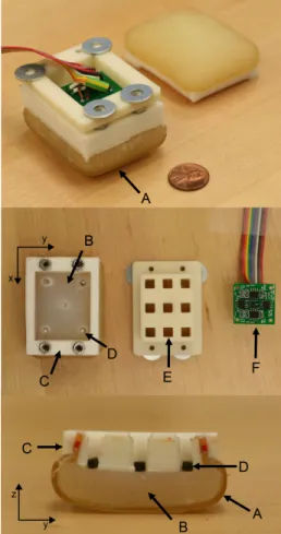
2-2 Assembled and disassembled force sensor. Components depicted

are (A) outer “skin” of woven fiberglass embedded in polyurethane rubber, (B) soft silicone rubber to form “padding” inside “skin”, (C) outer plastic for mounting and structure, (D) magnets mounted on top of silicone rubber, (E) ABS rigid well insert and (F) array of five Hall-effect sensors. In the bottom, cross-sectional view, a completely monolithic prototype was used, casting the outer wall and rigid wells

(C & E) as a single piece of Task® 4 plastic. . . 22

2-3 The current design of the footpad on the MIT Cheetah. The

top picture is of the MIT Cheetah and the bottom picture is of the footpad currently in use. The fabrication principle is the same, except

(10)

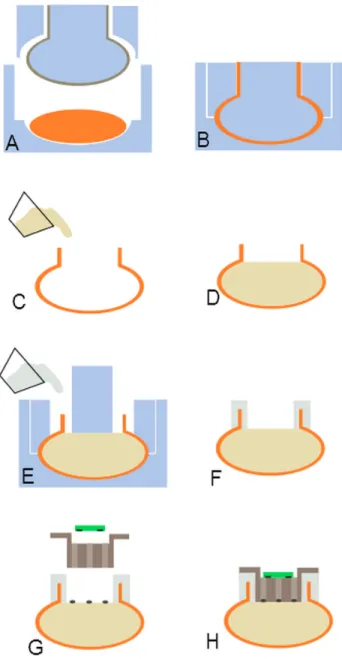
2-4 Cross-sectional view of fabrication process. Woven fiberglass is placed around a shaped insert (A) and pressed into a mold, embedding it within a tough, urethane rubber (B). Once removed, a soft silicone rubber is poured into the urethane casing (C & D). An outer, rigid lining is cast with urethane resin (E & F) which allows the rigid well insert and sensors to be mounted (G & H) after magnets are secured

to the top surface of silicone rubber. . . 26

3-1 Resistive Touch Screen Experimental setup and results . . . 29

3-2 FlexiForce Pressure Sensor Experimental setup and the voltage

comparator circuit . . . 30

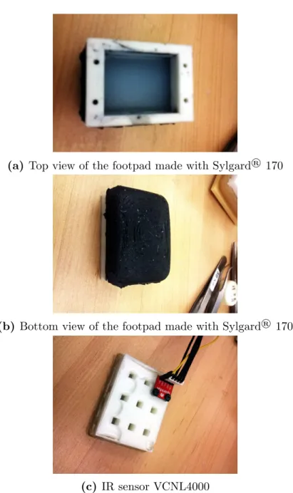
3-3 VCNL4000 IR Sensor and Sylgard® 170 The footpad of an

alter-native displacement sensing method using IR sensors being investigated. 32

3-4 Barometric Pressure Sensors The use of barometric pressure

sen-sors for force sensing being investigated. . . 34

3-5 Hall-effect Sensors The use of Hall-effect sensors for force sensing

being investigated. . . 36

5-1 Experimental setup with the materials testing machine.

Pre-liminary results were collected using a 6-axis F/T sensor (mounted beneath) to test the mechanism of volumetric displacement within the

footpad. . . 41

5-2 Experimental results for 10mm displacement in both X and

Y-axis. The top two graphs, (a) and (b), show the forces measured by the F/T sensor. The bottom two graph, (c) and (d), show the resulting

change in the MFD. All graphs show a 10s interval. . . 42

5-3 Experimental setup with the CNC milling machine. The foot

was mounted directly to the quill of the milling machine to ensure stiffness. The footpad made direct contact with the 6-axis force sensor

(11)

5-4 Two-axes shear training and testing paths. The two paths were used to train the ANN. The furthest points on each sub-trajectory correspond to a radius of 5mm away from the center of each path.

Both paths were run at several, set normal loads. . . 45

5-5 Experimental results for correspondence between the

pre-dicted force and actual force. The blue line shows the actual force measured and the red line shows the neural network predicted force. The figures are in the order of X, Y and Z-axis from top to bottom

respectively. . . 46

6-1 Angled InsertsInvestigating the effects of angled wells on the

sensi-tivity to shear forces . . . 50

6-2 Robotic Hand Prototype Preliminary investigation into the use of

hyperelastic materials in the fabrication of a robotic hand. . . 51

A-1 Closeup of the footpad showing the position of the 5 magnets. . . 56

A-2 Closeup of the assembled footpad showing the position of the 5

mag-nets. The piece above is the separate ABS insert. . . 56

A-3 A picture of the NI sbRIO 9642 used for data acquisition. . . 56

A-4 The outer ‘skin’ is made of a layer of fiberglass cloth coated in Vytaflex®20.

Once this layer cures, Ecoflex® 00-10A silicone rubber is poured into

(12)

(13)

List of Tables

2.1 Materials used in fabrication . . . 25

3.1 Properties of the tested barometric pressure sensors . . . 33

(14)

(15)

Chapter 1 Introduction

High speed running places great demands on the sensing capabilities of any robot, and this is especially true in the foot. As the sole interface between the robot and the ground, it is the only means with which a legged machine can generate reaction forces with its environment. In order to provide useful feedback and control, the ground contact model should be as accurate as possible. This means that the force sensor in the footpad should have a high dynamic range in both normal and shear for a complete picture of the reaction forces, all the while being tough enough to withstand the impact of repeated foot strikes during running. Indeed, durability is but one of a variety of functional requirements necessary from feet in general. The ability to adapt to asperities in the ground, absorb impacts, provide traction, and store and release energy are all important functions [6, 11]. Additionally, it has been shown that the viscoelastic properties of mammalian paw pads are critical in ensuring a desirable dynamic response under impacts such as those experienced during running [1]. This diversity of goals in an ideal foot presents a sensing problem that occupies a niche not readily addressed by off-the-shelf solutions.

Though tactile sensing has been the focus of much research within the field of robotics, current sensing methodologies are almost invariably designed separately from the robot itself, often utilizing standard components. This result in sensors that are ‘added-on’ to the robot instead of being built into the robot’s design, which can be problematic when designing systems for very specialized applications. When the

(16)

need for force sensing arises, what is ordinarily done is to add on sensing elements to the existing architecture of the robot. This can be in the form of strips of force sensitive resistors (FSR) on the external surfaces of the robot or force/torque (F/T) sensors at the joints.

1.1 Current Approaches to Integrating Sensing in

Robotics

The most conventional of approaches to force sensing fail to incorporate the compli-ance that is essential for successful interaction with terrain while running [1]. These methods have often taken a policy of separating a robot from its environment by placing the sensor directly between a robot and its foot. Reaction forces acting upon the machine are commonly rerouted and transmitted through the sensor to attain a measurement which ultimately alters the original mechanics. The gold standard, a traditional force/torque sensor, is one example of such a methodology that is com-monly found in industrial robotics and humanoid robots used for research. ‘KHR-3 Hubo’ [19] and ‘LOLA’ [15] are two examples of humanoid robots that use a custom F/T sensor in each foot for sensing ground contact. The direct use of F/T sensors for force sensing in the foot makes the foot much more bulky, weighing the robot down. This is not ideal, especially in the case of a robotic foot as it increases the ‘impact mass’ of the foot. A greater ‘impact mass’ is undesirable as it affects the sensing accuracy, particularly during high speed motion and potentially makes the robot less safe to work with. It is also not feasible to reduce the size of the F/T sensor as the F/T sensor needs to be of a certain strength and stiffness in order to measure the high forces of ground impact in a robotic foot. Similarly, ‘BIPMAN’ attempts to emulate the human foot, but still uses multiple off-the-shelf sensing solutions [11].

Furthermore, the broader approach of measuring the deformation of rigid struc-tures, as is done in F/T sensors, is less than ideal despite the allure of linearity and repeatability in measurements. Such a method would require the need for sensors to

(17)

be mounted far from the foot-ground contact with compliant mechanisms between the two or depend on a rigid contact surface with the ground that would likely result in chatter due to the large ‘impact mass’ [1]. In fact, having the sensor anywhere in series with the robot, the sensor may respond with undesired dynamics such as out-of-phase non-collocated modes, like chattering, during actuation. This poses problems for the controller, and may cause instabilities in the system [8].

1.2 Previous Work on Compliant Sensors Utilizing

Hyperelastic Materials

Compliant sensors take a different approach but often encompass many concerns sig-nificantly removed from those required from the demands of robotics. Scalability, adaptability to curved surfaces, low power consumption, and cost all aim to maxi-mize the sensors’ utility in a wide range of applications as a “artificial skin” [28, 13]. Phan et al. demonstrated the use of capacitive skin sensors to monitor the collisions and impact of a robot arm [24]. Likewise, tactile sensors for human gait analysis within medical studies seek to fill a similar niche but are constrained by the need to interface with existing footwear and measure many more parameters than are required for robotic running. As a result, the subsequent design integrates many different types of sensors and supporting hardware irrelevant to simply measuring ground reaction force and touchdown [17]. While this and other similar solutions are well suited for retroactively fitting robots with the ability to sense touch or compre-hensively measuring physiological parameters, there is still much to be desired. This is especially the case when considering the dynamic requirements of the footpad on a running, quadruped. It is desirable to extract only the essential measurements and minimize the demand put on the control system, which must compute in real-time during running. More sensors are almost always preferable to less sensors, but this leads to problems in signal acquisition. To pre-process the signal data and reduce the complexity, sensor fusion techniques can be used such as using artificial neural

(18)

networks as discussed in the later sections. The same too can be said of force sensing in a robotic hand, where the hand needs to compute the grip force applied and the occurrence of slippage in real-time.

Given the aforementioned challenges in matching off-the-shelf sensors to a very specialized application, designing the sensing solution in tandem with the robot can result in great advantages. For example, the musculoskeletal humanoid ‘Kojiro’ inno-vatively utilizes joint-angle sensors found in mobile phones in its spherical joints [29]. Another good example of this is seen in the custom-built strain sensor developed by Park et al. for use in their active soft orthotic device [21]. This is combined with their hyperelastic pressure sensor [22] to form a soft artificial skin with conductive liquid metal channels capable of multi-modal sensing [20]. Similarly, the exoskeletal end-effectors embedded with optical fiber Bragg grating sensors allowed Park et al. to integrate sensing while minimizing the bulkiness of hardware [23]. Wettels et al. have created a high performance biomimetic tactile finger (BioTac) with an incom-pressible conductive fluid surrounded by the elastomeric skin of the fingertip [30]. In this manner, they are able to use an array of electrodes to detect the deformations of the fingertip membrane. Further design of the skin texture enhanced the response of the finger [31]. Likewise, the technique of Electrical Impedance Tomography (EIT) is utilized by Alirezaei et al. in the creation of a highly stretchable tactile distribution sensor [2].

1.3 Specialized Application in Running Robots

The ideal sensor for use in the robotic foot would be one that closely mimics the many functions of biological human skin. The skin acts as a water-resistant barrier to protect the rest of the body from the environment. In the same way, the sensors in the robotic foot would need to be covered so as to function properly. The skin of the foot is especially thick for this reason. The human skin also has compliance due to the multilayer structure of the epidermis, dermis and hypodermis layers. This gives the skin compliance and allows it to conform to a variety of surface geometries. It

(19)

also contains a high density of mechanoreceptors in the dermis layer, right next to the outer epidermis layer [26]. The mechanoreceptors respond to touch and pressure, allowing human beings to have touch sensing capabilities all over their body. Note that the ‘impact mass’ of the human skin is almost negligible.

Figure 1-1: Mechanoreceptors in the human skin A section of the human skin showing the different types of mechanoreceptors (Ruffini endings, Merkel’s discs and Meissner’s corpuscles) in the dermis layer [26].

Drawing inspiration on the above examples, it is proposed here the fabrication of a novel integrated force sensor with applications in robotics. By integrating sensing directly into the design architecture of the robot, instead of as an afterthought, a robotic foot sensor can more closely resemble the architecture of the human skin. This can be done by using hyperelastic materials with embedded sensing elements in the fabrication of the robot. By using lightweight hyperelastic materials, the ‘impact mass’ of the robotic appendage is greatly reduced. Also the use of such materials gives the robot much needed compliance.

Due to the current limitations in sensing technologies, there is a need for a light-weight resilient force sensor for use in a running quadrupedal robot. In this thesis, we will introduce a light-weight force sensor integrated into the foot of a running

(20)

robotic quadruped that serves a dual purpose. The fabrication technique allows for a compliant footpad that will grip to most ground surfaces without wearing out quickly. The footpad also integrates an array of Hall-effect sensors and magnets which enables it to detect ground contact and shear. The design, construction, and characterization of the force sensor are further elaborated in later sections.

(21)

Chapter 2 Design and Fabrication of a

Robotic Footpad

The integrated, volumetric displacement force sensor utilizes the novel approach of sensing the deformation of a soft, elastomeric padding into an array of rigid wells, as depicted in Fig. 2-1. Small magnets are mounted onto the padding, which allows the proximity of the elastomers surface to be sensed by Hall-effect sensors placed above

Figure 2-1: Deformation of Elastomeric Padding within Foot Sensor. As ground reaction forces are applied to the footpad in this cross-sectional view, the soft elastomer deforms up into the rigid wells, sending a unique signal, based on the normal and shear components, to the Hall-effect sensors mounted above.

(22)

these wells. As the wells are part of a single elastomer, any shear on the foot will affect the individual wells and magnets differently. This results in a change in the Magnetic Flux Density (MFD), which is then recorded via the Hall-effect sensors. Using neural networks to calibrate the system once, the MFD is related to the measured normal and shear forces. The geometry of the base of the footpad is intentionally curved so as to amplify the differences in the wells and to avoid simple shear from occurring. A photo of the monolithic foot structure, the rigid well insert, and Hall-effect sensors mounted onto a printed circuit board (PCB) are shown assembled and disassembled in Fig. 2-2, along with the cross-section of a completely monolithic iteration.

Figure 2-2: Assembled and disassembled force sensor. Components depicted are (A) outer “skin” of woven fiberglass embedded in polyurethane rubber, (B) soft silicone rubber to form “padding” inside “skin”, (C) outer plastic for mounting and structure, (D) magnets mounted on top of silicone rubber, (E) ABS rigid well insert and (F) array of five Hall-effect sensors. In the bottom, cross-sectional view, a completely monolithic prototype was used, casting the outer wall and rigid wells (C & E) as a single piece of Task® 4 plastic.

(23)

2.1 Foot Design

This current foot design has gone through multiple design iterations and has demon-strated robust performance with our MIT Cheetah, a quadrupedal robotic platform intended to test high speed running (Fig. 2-3). The biomimetic design was inspired by the texture and shape of feline paws. This work serves to incorporate the volumetric displacement sensing principle into the current design to allow for force sensing.

Several aspects were incorporated into the design of the foot in order to promote successful interaction with the ground. Firstly, the tougher, outer “skin” of the foot

was cast using a durable rubber, Vytaflex® 20, in order to withstand the wear and

tear that repeated impact and loading would impose on the material. The rubber material provided a high coefficient of friction to generate sufficient forces tangent to the ground during contact.

Woven fiberglass was embedded within the outer, rubber layer to strengthen it against strain in the surface area of the pad. This resistivity to strain strengthens the pad to shear forces but keeps the foot compliant to forces acting normal to its surface. This directional compliance further facilitates the driving mechanism utilized by the sensor, as the soft elastomer is prevented from slipping out from under the foot due to shear, but uninhibited from being pushed up inside the rigid wells when loaded under normal forces. The compliant pad also lowers peak forces experienced by the foot and acts as a mechanical, low-pass filter for asperities in the ground. The compliance allows the foot to simply deform around smaller asperities in the ground that would trouble rigid structures.

Our design of having the volumetric displacement sensor integrated into the foot-pad means that the amount of mass in series after the sensing unit available to give rise to instabilities is minimal. Other unwanted dynamic effects are also avoided, such as noise due to inertial factors during periods of high acceleration. In the current design, only 35 grams of mass is present between the sensor and the ground.

(24)

2.2 Fabrication Technique

The sensor was fabricated by casting several different thermosetting polymers to one another. The monolithic design was chosen to promote robustness during impact, and minimize the size the sensing unit occupied. As an added bonus, since the sensor is completely encased in the footpad, it is protected from the environment and unlikely to fail. An illustrated overview of the process can be seen in Fig. 2-4.

The tough, outer “skin” of the foot was constructed by embedding woven fiberglass

into a 2mm thick layer of Vytaflex® 20 polyurethane rubber of Shore hardness 20A.

After demolding, the skin retained the shape imposed by the casting process and was

filled with Ecoflex® 00-10 Supersoft Silicone rubber of Shore hardness 00-10A, which

was allowed to self-level.

A rigid, outer lining was cast on top of these rubbers using Task® 4 polyurethane

resin of Shore hardness 83D. The rigid lining provided structural integrity and allowed for a separate insert to be anchored onto the foot which imposed the rigid wells above the silicone rubber. The insert is made out of acrylonitrile butadiene styrene (ABS) and can be quickly redesigned and printed in a conventional 3D printer. The use of a separate insert allowed for rapid iteration on the geometry of the wells and greater ease in securing the magnets to the soft, silicone rubber. Additional figures of the intermediate steps in fabrication can be found in the Appendix A. Ultimately, the

ABS insert would be replaced by casting the well geometry directly into the Task®4,

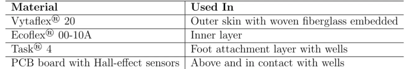
once an optimal configuration had be conferred upon. This is summarized in Table 2.1.

The final weight of the full prototype with ABS insert was 95 grams, while com-pletely monolithic iterations weighed only 60 grams where the wells were cast directly

(25)

Material Used In

Vytaflex® 20 Outer skin with woven fiberglass embedded

Ecoflex® 00-10A Inner layer

Task® 4 Foot attachment layer with wells

PCB board with Hall-effect sensors Above and in contact with wells

Table 2.1: Materials used in fabrication

Figure 2-3: The current design of the footpad on the MIT Cheetah. The top picture is of the MIT Cheetah and the bottom picture is of the footpad currently in use. The fabrication principle is the same, except that there are 2 separate pads and it lacks force sensing capabilities.

(26)

Figure 2-4: Cross-sectional view of fabrication process. Woven fiberglass is placed around a shaped insert (A) and pressed into a mold, embedding it within a tough, urethane rubber (B). Once removed, a soft silicone rubber is poured into the urethane casing (C & D). An outer, rigid lining is cast with urethane resin (E & F) which allows the rigid well insert and sensors to be mounted (G & H) after magnets are secured to the top surface of silicone rubber.

(27)

Chapter 3 Sensor Design

In order to measure force, it must be converted into a quantity that can readily be measured as a signal. The deformation of the soft elastomer within the paw pad was chosen as the sensing mechanism. This required no additional mass to the foot but rather hollowing out wells in the rigid, plastic structure of the top of the foot while inserting small magnets and Hall-effect sensors into the structure. The chosen mechanism incorporates the compliance necessary to facilitate successful interaction with terrain, and minimizes need for additional weight or components, and allows for a monolithic and robust structure. The presented sensor strives to attain a greater level of integration within a compliant structure in order to preserve the original design intent and promote dynamics favorable to running while measuring ground reaction forces as close to the foot-ground interface as possible.

Other mechanisms for measuring the ground reaction forces were also investigated, but these were eventually cast aside in favor of the current approach of using magnets and Hall-effect sensors.

3.1 FSR Sensors

One initial idea was the use of force sensitive resistors (FSR) as the force sensing element in the footpad. A force sensitive resistor is made of two layers of conduc-tive electrodes sandwiching a layer of conducconduc-tive polymer. The conducconduc-tive polymer

(28)

changes resistance when a force is applied to it. This change in resistance is then

mea-sured by the electrodes. A 4 wire resistive touch screen from a Nintendo DS® was

used as it provided both the force magnitude as well as the location of the peak force

in two axes. An Arduino® Nano microcontroller was used to interface with the

resis-tive touch screen and send the data to MATLAB® for processing as shown in Fig.

3-1. While proved to work well in determining the location of the maximum force with high sensitivity, the sensor also saturated under forces of 10N or less. Also the accuracy of the sensor was low, usually on the order of 10% error.

The next step was to use FSRs with higher force ranges and to use it as a binary

ground contact sensor. After some trials with a variety of FSRs from Tekscan® ,

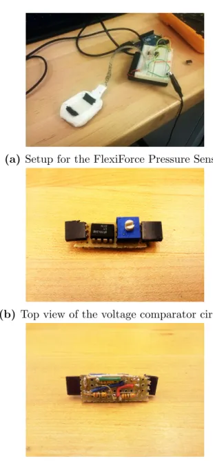
the FlexiForce® Pressure Sensor was chosen for its flexibility, robustness, accuracy

of around 3% and high force range of up to 100lbs. The FSR was then embedded into the new footpad design to validate the performance. Using a high-speed voltage comparator LM311 and a potentiometer, an electrical circuit was constructed to bias the output of the FSR such that on ground contact, the output voltage of the LM311 would go high to +5V and in the air, it would drop to 0V. This circuit was prototyped as shown in Fig. 3-2.

While the FlexiForce FSR in conjunction with the voltage comparator LM311 circuit allowed the footpad to detect the occurance of ground contact, the output remained high ever after the foot left the ground for a few milliseconds. It is

hypoth-esized that this is caused by the adhesion of the sensor to the Ecoflex® 00-10A layer

in the footpad. This makes it difficult to determine the duration of ground contact which causes problem for the robot controller.

3.2 IR Sensors

Another sensing mechanism that was explored was the use of infrared (IR) sensors. IR sensors measures distances by sending out a pulse of IR light which bounces off a surface and is received by an IR receiver. Based on the time of flight, the distance between the IR sensor and the surface can be determined.

(29)

(a) Setup for the Resistive Touch Screen

(b) MATLAB data from the Resistive Touch Screen

(30)

(a) Setup for the FlexiForce Pressure Sensor

(b) Top view of the voltage comparator circuit

(c) Bottom view of the voltage comparator circuit

Figure 3-2: FlexiForce Pressure Sensor Experimental setup and the voltage com-parator circuit

(31)

The volumetric displacement sensing method does not have to rely on a combi-nation of Hall-effect sensors and magnets. IR sensors can be used to determine the displacement of the hyperelastic gel material into the wells of the footpad. However, this method is susceptible to interference in the form of ambient light in the envi-ronment. Some preliminary investigations were conducted in this direction. The

IR sensor used is the VCNL4000 from Vishay® Semiconductors. Data was

col-lected using an Arduino® Nano microcontroller to interface with the IR sensor

through Inter-Integrated Circuit (I2_{C) communications protocol. With the}

translu-cent Vytaflex® 20 ‘outer skin’, the IR sensor gave inconsistent readings due to the

varying amounts of incident ambient light. The I2_{C protocol also limited the speed}

at which data could be transmitted. An attempt was made to fixed this by using

Sylgard® 170, an opaque black silicone elastomer with a Shore hardness of 43A. It is

used in the place of the Vytaflex® 20 polyurethane rubber in the outer ‘skin’ layer to

prevent ambient light from leaking into the sensor. Future work includes fabrication a PCB for an array of IR sensors and further tests on using a cheaper phototransistor QRD1114 with direct analog output to increase the communications speed.

(32)

(a) Top view of the footpad made with Sylgard® 170

(b) Bottom view of the footpad made with Sylgard® 170

(c) IR sensor VCNL4000

Figure 3-3: VCNL4000 IR Sensor and Sylgard® 170 The footpad of an

(33)

3.3 Barometric Pressure Sensors

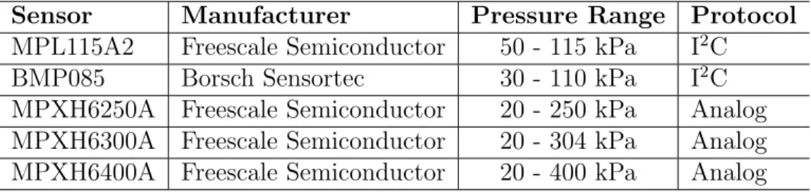
The idea of using MEMS barometric pressure sensors for force sensing came from the Harvard Biorobotics Laboratory under the open-source project ’TakkTile’ [27]. The approach used is to attach barometric pressure sensors onto PCBs and then pour urethane rubber over the sensors. Then before the urethane rubber has time to cure, the sensors are placed in a vacuum chamber to draw all the trapped air out. This step is called degassing and it brings the urethane rubber in contact with the pressure sensor’s diaphragm. By doing this, the sensor is protected from the envi-ronment and it increases the force sensing range as well. TakkTile uses MPL115A2 minature digital barometers by Freescale Semiconductor. This is unsuitable for our intended application in the footpad as the MPL115A2 has a low pressure range which

corresponds to a lower force range. It also uses the I2_{C protocol which requires an}

additional microchip to handle the addressing. Hence four other barometric pressure sensors are investigated, as summarized in Table 3.1.

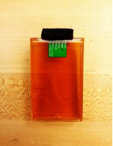
The sensors were embedded in Vytaflex® 60 polyurethane rubber and degassed.

An Arduino®Nano microcontroller was then used to collect the voltage data from the

barometric pressure sensors. As shown in Fig. 3-4c, the sensors show an almost linear relationship between the output voltage and applied force. Empirically, the pressure sensors in the ’port’ package performed much more poorly than the flat package ones. The sensors also suffer from drift issues which might have some temperature

dependancy. There were also creep effects from the compression of the Vytaflex® 60

rubber.

Sensor Manufacturer Pressure Range Protocol

MPL115A2 Freescale Semiconductor 50 - 115 kPa I2C

BMP085 Borsch Sensortec 30 - 110 kPa I2C

MPXH6250A Freescale Semiconductor 20 - 250 kPa Analog

(34)

(a) Embedding the pressure sensor (BMP085 in this case) in Vytaflex® 60

(b) Experimental setup of the cured pressure sensors

(c) Data from one of the pressure sensors

Figure 3-4: Barometric Pressure Sensors The use of barometric pressure sensors for force sensing being investigated.

(35)

3.4 Hall-effect Sensors

For the preliminary research into the use of Hall-effect sensors in the volumetric

dis-placement sensing principle, SS495A Hall-effect sensors from Honeywell® were used.

The sensors were mounted in a square array and soldered onto a piece of protoboard.

Once again, data from the sensors were collected using an Arduino® Nano

microcon-troller and plotted in MATLAB®. In Fig. 3-5c, the sensor was manually stimulated

using a tiny (2.5mm diameter by 0.8mm thick) disc magnet. It can be clearly seen that the Hall-effect sensor is able to pick up the weak magnetic field of the tiny disc magnet. Due to the high signal-to-noise ratio and the ease of using the Hall-effect sensors, the choice was made to use them as the sensing element in the footpad. However, the sensors are still susceptible to noise from electromagnetic interference as will be seen in the later sections.

(36)

(a) Top view of the SS495A Hall-effect sensor array

(b) Bottom view of the SS495A Hall-effect sensor array

(c) Data from one of the SS495A Hall-effect sensors

Figure 3-5: Hall-effect Sensors The use of Hall-effect sensors for force sensing being investigated.

(37)

Chapter 4 Artificial Neural Networks and

Force-Deformation Relation

4.1 Artificial Neural Networks

Artificial Neural Networks (ANN) draw their inspiration from biological neural net-works, such as the interconnected neurons found in an animal’s nervous system. Sim-ilarly, an artificial neural network is made up of artificial neurons connected together in different layers with various interconnects. An ANN is usually constructed with a structure of g hidden layers and h hidden nodes which determines the order of the network. This enables the ANN to manage multiple inputs and outputs and to deduce the complex relationships between them.

Using supervised learning, an artificial neural network can be trained. This means that the ANN will attempt to find an objective function that maps the inputs to the outputs of the data. This is done by iteratively adjusting the weights of each individual artificial neuron in the network. The error in this case is the difference between the ANN outputs and the know outputs provided in the data. A commonly used cost function to minimize this error is the root mean squared (RMS) error.

Due to the complexity in the geometry of the footpad and the elastomer, attaining analytical models through the use of hyperelastic material models is non-trivial. The total force can be estimated by assuming that the footpad is a rectangular block

(38)

of elastomeric material with various material models such as Mooney-Rivlin [25], Arruda-Boyce [4] and Ogden [18]. These models are highly dependent on the quality

of the experimental data collected. The difficulty is furthered with the presence

of wells that the elastomer deforms into and the use of two different elastomers in

each layer (Vytaflex® 20 and Ecoflex® 00-10). Additionally, the magnetic fields are

coupled, making the use of a single dipole model unsuitable. This makes it almost impossible to predict the change in height and orientation of the magnets in the wells. Simulating the footpad deformations using a finite-element analysis package such

as Abaqus was considered, but the resulting model was overly complex and took an

unreasonable amount of time to solve for a set of initial conditions. Similarly, the accuracy of the model depends greatly on the material properties that are obtained

experimentally. Hence, a more straightforward method was sought. In the end,

the use of an artificial neural network (ANN) to directly associate the forces with the Magnetic Flux Density (MFD) was determined to be the best way to obtain the correlation. It offers the advantages of only requiring a one-time calibration procedure and is able to provide force feedback to the system in real-time.

4.2 Sensor PCB Board

A small 1 inch by 1 inch PCB was manufactured and populated with 5 single-axis

Hall-effect sensors. The center sensor is an Asahi EQ-430L (S0) and 4 Sentron

CSA-1VG sensors (S1, S2, S3 and S4) surround it with the sensing axis aligned to the X

and Y-axis as seen in Fig. 2-2. Each peripheral sensor is separated by a distance of 7.5mm from the central sensor and this orientation allows each sensor to pick up the slight changes in the MFD during ground contact. The overall change in the MFD can be summarized by the function below:

SM DF(t) = [S0(t) . . . Si(t) . . . S4(t)]T (4.1)

where Si is the individually measured MFD of the ith magnetic sensor. In this

(39)

the surface of the hyperelastic gel-like pad. The vector SM F D(t) can be represented

by either an analytical distributed multipole model [14] or through experimental field measurements.

4.3 Force-Deformation Relation

This PCB is then mounted over the wells containing the magnets (Grade N42). As the magnets are connected by a monolithic piece of elastomer, any normal forces will cause the 4 magnets near the edges to rise by the same amount. However, in the case of shear forces, the wells along the outer edges deform by different amounts and these discrepancies are picked up by the Hall-effect sensors on the PCB. The loading conditions on the footpad are measured by a F/T sensor and can be represented as:

F (t) = [FX(t) FY(t) FZ(t)]T (4.2)

where Fi (t) is the recorded force in each respective axis. This change in the

MFD, SM F D(t) is then parsed in MATLAB and the MFD and the applied forces

are empirically correlated using the Neural Network Toolbox. A feed-forward neural network is created where an input-output relationship is mapped between the MFD as measured by the 5 Hall-effect sensors and the forces recorded by a F/T sensor. The Levenberg-Marquardt optimization network training function [16] then uses a back-propagation algorithm to update the weights and bias values of the neural network until the minimum mean squared error is obtained and the desired performance is realized. Note that the Levenberg-Marquardt algorithm, or damped least-squares method, is an example of a nonlinear regression algorithm. The Levenberg-Marquardt algorithm is given as:

[JTW J + λdiag(JTW J )]δ = JTW [F (t) − ˆF (t)] (4.3)

where J is the gradient matrix, W is the weighting matrix, λ is the algorithmic parameter, δ is the increment in each iteration, F (t) is the target force output from

(40)

the F/T sensor and ˆF (t) denotes the force estimates of the ANN. This method on the use of artificial neural networks for force sensing is further elaborated on in the previous work done by Ananthanarayanan et al. [3].

(41)

Chapter 5 Experimental Results

5.1 One Axis Results

Preliminary results were generated with one-axis machine in order to assess the pro-totypes potential in both normal and shear directions.

The footpad sensor was first clamped into the top jaws of an industrial

materials-testing machine (Zwick Roell BX1-EZ005.A4K-000) with a manual 2-axis table

loaded onto it. A 6-axis F/T sensor (ATI Industrial Automation SI-660-60) was

mounted to the base of the materials testing machine which is capable of measuring up to 1980N in the Z-axis with a resolution of 0.25N. The footpad was lowered onto the F/T sensor until the desired normal force was reached. This experimental setup

Figure 5-1: Experimental setup with the materials testing machine. Prelim-inary results were collected using a 6-axis F/T sensor (mounted beneath) to test the mechanism of volumetric displacement within the footpad.

(42)

(a) Forces in X-axis (b) Forces in Y-axis

(c) MFD in X-axis (d) MFD in Y-axis

Figure 5-2: Experimental results for 10mm displacement in both X and Y-axis. The top two graphs, (a) and (b), show the forces measured by the F/T sensor. The bottom two graph, (c) and (d), show the resulting change in the MFD. All graphs show a 10s interval.

can be seen in Fig. 5-1. The data from the volumetric displacement footpad sensor and the F/T sensor are acquired through a National Instruments Single-Board RIO

(NI sbRIO 9642) connected through LabVIEW. This setup allowed for arbitrary

normal loading conditions while shear in both the X and Y-axis is observed. The axes are depicted in Fig. 2-2.

Using the above setup, the footpad was preloaded with a normal force using the materials testing machine and then the 2-axis table was then manually actuated by the researcher in both the X and Y-axis by 10mm. This is done at a rate of around 1.5 Hz. The results are shown in Fig. 5-2. The results show that there is a good correspondence between the MFD changes and shear in the X-axis but less so for

shear in the Y-axis. The MATLAB® code used to generate the results can be found

(43)

5.2 Combined Two Axes Shear Results

In order to get training data to feed into the neural network, accurate linear position-ing of the footpad is required. This was achieved by usposition-ing an industrial 3 axis CNC

milling machine (HAAS Super Mini Mill 2). A mount was fabricated to attach the

footpad directly to the quill and a separate mount for attaching the F/T sensor to the mill table. This experimental setup is shown in Fig. 5-3. A picture of the NI

sbRIO 9642 used for data acquisition can be seen in Appendix A.

Training data was first collected by having the CNC milling machine run through a programmed training path with the footpad in contact with the F/T sensor. With a known normal load, the footpad was made to traverse 5mm in both the positive and negative directions along the X-axis. This was then repeated in the Y-axis. Finally, the footpad was made to follow a circular path of 10mm diameter about the origin. For verification, the more data was gathered with an arbitrary path. This path involved a diagonal motion of 5mm in each of the 4 quadrants of the X and Y-axis. This was then followed with 4 smaller circular paths of 5mm diameter along

Figure 5-3: Experimental setup with the CNC milling machine. The foot was mounted directly to the quill of the milling machine to ensure stiffness. The footpad made direct contact with the 6-axis force sensor during testing.

(44)

Axis Force Magnitude (N) RMS Error (N)

X-axis 40 16.76

Y-axis 40 12.90

Z-axis 80 4.83

Table 5.1: Result of the combined two axes experiment

each of the positive and negative X and Y-axis. A qualitative depiction of the paths is shown in Fig. 5-4.

The results (Fig. 5-5) show that the neural network is able to predict normal forces in the Z-axis up to 80N with the greatest accuracy. The root mean squared (RMS) error is 4.83N. This represents a RMS error of 6.04%. This is followed by the Y-axis where shear forces of 40N are detectable, but the predicted force magnitude does not correspond with reality completely. The RMS error in this case is 12.90N. In the X-axis, similar performance is observed where shear forces of up to 40N are predictable, but the force magnitudes differ. The RMS error for the X-axis is 16.76N. These results are summarized in Table 5.1. Note that the noise levels in these graphs

are much higher than the ones for the previous setup in Fig. 5-1. This is due

to electromagnetic interference (EMI) from the CNC milling machine, and would inevitably improve in environments more natural to running. A Butterworth filter with a 10Hz cutoff frequency has been applied to the gathered signals to remove

the EMI noise. The MATLAB® code used to generate the results can be found in

(45)

Figure 5-4: Two-axes shear training and testing paths. The two paths were used to train the ANN. The furthest points on each sub-trajectory correspond to a radius of 5mm away from the center of each path. Both paths were run at several, set normal loads.

(46)

(a) Forces in X-axis

(b) Forces in Y-axis

(c) Forces in Z-axis

Figure 5-5: Experimental results for correspondence between the predicted force and actual force. The blue line shows the actual force measured and the red line shows the neural network predicted force. The figures are in the order of X, Y and Z-axis from top to bottom respectively.

(47)

Chapter 6 Discussion and Future Works

The proposed design offers a method to marry two distinct goals in foot design for running applications: promoting favorable dynamic performance and extracting an accurate measurement from ground reaction forces. Both can be accomplished in a robust manner while minimizing weight and number of parts by integrating them completely. In order to do so in a manner that does not severely restrict design space, the mechanical considerations of the footpad and the considerations given to the mechanisms utilized by sensor are effectively decoupled through the use of the ANN. Thus, the dynamic response can be designed and achieved first while sensing is attained once the physical structure is established. In the specific case of the MIT Cheetah, a proven foot using this fabrication structure had already been developed and utilized in currently running experiments (Fig. 2-3). The end goal is to have sensing capabilities were efficiently integrated to the structure with minimal addition of hardware.

The experimental results show that the footpad sensor is able to detect normal loading conditions with sufficient accuracy and to identify the onset of shear in both the X and Y-axis. These results present a promising proof-of-concept on a novel mechanism to sense ground reaction forces while utilizing an inherently compliant interface with the terrain. However, several aspects of the design are readily available for improvement within subsequent iterations as well.

(48)

6.1 Additional Training Data

Collecting additional training data may further fine-tune the ANN parameters and will allow us to minimize the errors in the force sensing. Only one group of trajecto-ries, repeated at varying normal loads, was used to produce the current correlation. There might be some load history dependence (e.g. creep effects) which needs to be investigated further. Specifically, impact tests may prove to be the most relevant training method for running and would provide more telling information such as re-sponse time. Unfortunately, the existing experimental setups do not readily allow for such tests to be conducted

6.2 Magnet Placement

The placement of the magnets, especially the direction of the poles should be modeled to achieve an optimal MFD that would give the maximum change in response to stress and shear. Foong et al. have used a network of Hall-effect sensors and magnets to obtain angular positional sensing by training the system with an ANN. They have shown that they are able to get a much higher degree of positional accuracy (up to nanodegrees) when using unevenly spaced sensors in a staggered configuration [10]. Arranging the magnets in the manner of a Halbach array might give rise to greater sensitivity [12]. This has the advantage of maximizing the magnetic field on the side facing the Hall-effect sensors. It also minimizes any stray fields on the ground-facing side, reducing the potential for interference from unintended sources. The size and shape of the magnets can be optimized as well.

6.3 Angled Inserts

In order to significantly improve the measurement of shear forces, alternative well geometries can be easily explored by 3D printing different ABS inserts. Rather than completely vertical extruded cuts, incorporating angled wells that travel some dis-tance along the X and Y axes may increase sensitivity and accuracy to shear forces.

(49)

Estrada et al. have obtain some promising results in exploring this area [9]. With the angled inserts, the overall qualitative trends are clearer especially for the shear directions in the X and Y-axis. However, the quantitative accuracy suffers with the angled inserts. Further experimentation is warranted to find the sources of the higher RMS error.

(a) Setup for the angled inserts

(b) SolidWorks® model of the angled inserts

Figure 6-1: Angled InsertsInvestigating the effects of angled wells on the sensitivity to shear forces

6.4 Variety in Hyperelastic Polymers

By varying the material properties of the hyperelastic gel-like pad, different force sensitivities can be achieved. This can be incorporated into the current ‘2-pad design (Fig. 2-3) where a single footpad will have 2 gel-like pads of different stiffness. The will allow the footpad to have a wider dynamic force range.

(50)

6.5 Force Sensing in Robotic Grippers

Robotic grippers commonly have multiple appendages so as to conform to a wide variety of object geometries. It is also necessary for the robotic hand to be able to sense the object being manipulated. The ability to sense forces would allow the robotic hand to grasp objects of different hardness without applying overly large forces and damaging them, and also allow for slip detection. As it is challenging to cover multi-fingered robotic hands with sensing elements, most designs concentrate on only having a passive force sensitive finger tip. However, this means that it is still possible for the robot to exert too much force when gripping objects with complex shapes. A better approach would be to integrate force sensitive elements throughout the robotic hand. Both the SDM hand by Dollar et al. [7] and the Robonaut 2 hand [5] have used this design approach to great success. Fig. 6-2 shows a prototype robotic hand made of hyperelastic materials with hinged joints. Each finger is made from a different

urethane rubber, such as Vytaflex® 10 and Vytaflex® 20 polyurethane rubbers of

Shore hardness 10A and 20A respectively, Ecoflex® 00-30 Supersoft Silicone rubber

of Shore hardness 00-10A and Dragon Skin® 10 High Performance Silicone rubber of

Shore hardness 10A. The barometric pressure sensing principle investigated in Section can be easily integrated into the pads of each finger segment.

Figure 6-2: Robotic Hand Prototype Preliminary investigation into the use of hyperelastic materials in the fabrication of a robotic hand.

(51)

Chapter 7 Conclusions

This thesis presents a proof-of-concept dual purpose footpad with integrated force sensing capabilities. The design of the footpad makes use of the strengths of 3 different polymers to give a footpad that is durable under repeated ground impacts while still being compliant enough to offer good traction. The volumetric displacement sensing principle utilizes a hyperelastic gel-like pad with embedded magnets, which allows normal and shear forces to be detected indirectly without the need to expose the sensor. A one-time training process using an artificial neural network is all that is necessary to relate the normal and shear forces with the volumetric displacement sensor output. The volumetric displacement sensor is able to detect normal forces up to 80N with a RMS error of 6.04% and the onset of shear forces in both the X and Y axis. This is a robust footpad sensor suitable for use in all outdoor conditions. Upon further refinements, this footpad is intended for use in the MIT Robotic Cheetah to detect the occurrence of ground contact and the forces involved.

(52)

(53)

Appendix A

Additional Figures

(54)

Figure A-2: Closeup of the assembled footpad showing the position of the 5 magnets. The piece above is the separate ABS insert.

(55)

(a) Top view of just the outer ‘skin’

(b) Bottom view of just the outer ‘skin’

(c) The outer ‘skin’ filled with silicone rubber

Figure A-4: The outer ‘skin’ is made of a layer of fiberglass cloth coated in Vytaflex® 20. Once this layer cures, Ecoflex® 00-10A silicone rubber is poured into the cavity and allowed to level.

(56)

(57)

Appendix B

MATLAB

®

Code

B.1 Code for the One Axis Results

c l o s e a l l; c l e a r a l l; c l c; T _ s t a r t = 1 0 0 0 0 ;

T _ e n d = 1 9 9 0 0 ;

%% Import e x c e l d a t a

F o r c e X = i m p o r t d a t a (' Force Y 0 −100 Trial 5 New . x l s x ', ' \ t ', 1 ) ; F o o t X = i m p o r t d a t a (' Foot Y 0 −100 Trial 5 New . x l s x ', ' \ t ', 1 ) ;

% ForceY = i m p o r t d a t a (' Force Y 0 −100. xlsx ' , '\ t ' , 1) ; % FootY = i m p o r t d a t a (' Foot Y 0 −100. xlsx ' , '\ t ' , 1) ; %% F o r c e from X−a x i s d i s p l a c e m e n t FxX = F o r c e X . d a t a ( T _ s t a r t : T_end , 2 ) ; FyX = F o r c e X . d a t a ( T _ s t a r t : T_end , 4 ) ; FzX = F o r c e X . d a t a ( T _ s t a r t : T_end , 6 ) ; TxX = F o r c e X . d a t a ( T _ s t a r t : T_end , 8 ) ; TyX = F o r c e X . d a t a ( T _ s t a r t : T_end , 1 0 ) ; TzX = F o r c e X . d a t a ( T _ s t a r t : T_end , 1 2 ) ;

%% Mag from X−a x i s d i s p l a c e m e n t

M a g X 1 = F o o t X . d a t a ( T _ s t a r t : T_end , 2 ) ;

% MagX2 = FootX . d a t a ( T s t a r t : T end , 4 ) ;

M a g X 3 = F o o t X . d a t a ( T _ s t a r t : T_end , 6 ) ;

% MagX4 = FootX . d a t a ( T s t a r t : T end , 8 ) ;

(58)

% MagX6 = FootX . d a t a ( T s t a r t : T end , 1 2 ) ;

M a g X 7 = F o o t X . d a t a ( T _ s t a r t : T_end , 1 4 ) ;

% MagX8 = FootX . d a t a ( T s t a r t : T end , 1 6 ) ;

M a g X 9 = F o o t X . d a t a ( T _ s t a r t : T_end , 1 8 ) ;

%% F o r c e from Y−a x i s d i s p l a c e m e n t % FxY = ForceY . d a t a ( T s t a r t : T end , 2 ) ; % FyY = ForceY . d a t a ( T s t a r t : T end , 4 ) ; % FzY = ForceY . d a t a ( T s t a r t : T end , 6 ) ; % TxY = ForceY . d a t a ( T s t a r t : T end , 8 ) ; % TyY = ForceY . d a t a ( T s t a r t : T end , 1 0 ) ; % TzY = ForceY . d a t a ( T s t a r t : T end , 1 2 ) ; %

%% Mag from Y−a x i s d i s p l a c e m e n t

% MagY1 = FootY . d a t a ( T s t a r t : T end , 2 ) ; % % MagY2 = FootY . d a t a ( T s t a r t : T end , 4 ) ; % MagY3 = FootY . d a t a ( T s t a r t : T end , 6 ) ; % % MagY4 = FootY . d a t a ( T s t a r t : T end , 8 ) ; % MagY5 = FootY . d a t a ( T s t a r t : T end , 1 0 ) ; % % MagY6 = FootY . d a t a ( T s t a r t : T end , 1 2 ) ; % MagY7 = FootY . d a t a ( T s t a r t : T end , 1 4 ) ; % % MagY8 = FootY . d a t a ( T s t a r t : T end , 1 6 ) ; % MagY9 = FootY . d a t a ( T s t a r t : T end , 1 8 ) ; %% P l o t d a t a

t = T _ s t a r t : 1 : T _ e n d ; t = t . / 1 0 0 0 ;

%% X−a x i s

% f i g u r e ; p l o t ( t , MagX1 , t , MagX2 , t , MagX3 , t , MagX4 , t , MagX5 , t , MagX6 , t , MagX7 , t , MagX8 , t , ←-MagX9) ; g r i d on ; l e g e n d (' Mag1 ' , ' Mag2 ' , ' Mag3 ' , ' Mag4 ' , ' Mag5 ' , ' Mag6 ' , ' Mag7 ' , '

Mag8←-' , Mag8←-' Mag9 Mag8←-' ) ; t i t l e ( Mag8←-'Mag from X−a x i s displacement Mag8←-' ) ;

f i g u r e; p l o t( t , FxX , t , FyX , t , FzX , t , TxX , t , TyX , t , TzX ) ; g r i d on ; l e g e n d('Fx ','Fy ',' Fz ',

'←-Tx','Ty ','Tz ') ; x l a b e l(' Time ( s ) ') ; y l a b e l(' Force (N) ') ;

f i g u r e; p l o t( t , MagX1 , t , MagX3 , t , MagX5 , t , MagX7 , t , MagX9 ) ; g r i d on ; l e g e n d(' S1 ',' S2 ',

'←-S3',' S4 ',' S0 ') ; x l a b e l(' Time ( s ) ') ; y l a b e l(' Voltage (V) ') ;

% s u b p l o t ( 2 , 1 , 2 ) , p l o t ( t , MagX3 , t , MagX5 , t , MagX7 , t , MagX9) ; g r i d on ; l e g e n d (' Mag3 ' , ' ←-Mag5' , ' Mag7 ' , ' Mag9 ' ) ;

% f i g u r e ; p l o t ( t , FxX,' −x ' , t , FyX, ' −o ' , t , FzX, ' −+ ' , t ,TxX, t ,TyX, t , TzX, t , MagX1, t , MagX3, t ←-, MagX5 ←-, t ←-, MagX7 ←-, t ←-, MagX9) ; g r i d on ; l e g e n d (' Fx ' , ' Fy ' , ' Fz ' , ' Tx ' , ' Ty ' , ' Tz ' , ' Mag1 ' , ' ←-Mag3' , ' Mag5 ' , ' Mag7 ' , ' Mag9 ' ) ; t i t l e ( ' Force and Mag from X−a x i s displacement ' ) ; %% Y−a x i s

(59)

% f i g u r e ; p l o t ( t , MagY1 , t , MagY2 , t , MagY3 , t , MagY4 , t , MagY5 , t , MagY6 , t , MagY7 , t , MagY8 , t , ←-MagY9) ; g r i d on ; l e g e n d (' Mag1 ' , ' Mag2 ' , ' Mag3 ' , ' Mag4 ' , ' Mag5 ' , ' Mag6 ' , ' Mag7 ' , '

Mag8←-' , Mag8←-' Mag9 Mag8←-' ) ; t i t l e ( Mag8←-'Mag from Y−a x i s displacement Mag8←-' ) ; % f i g u r e ;

% s u b p l o t ( 2 , 1 , 1 ) , p l o t ( t , FxY , t , FyY , t , FzY , t , TxY, t , TyY, t , TzY) ; g r i d on ; l e g e n d (' Fx ' , ' ←-Fy' , ' Fz ' , ' Tx ' , ' Ty ' , ' Tz ' ) ; t i t l e ( ' Force from Y−a x i s displacement ' ) ;

% % s u b p l o t ( 2 , 1 , 2 ) , p l o t ( t , MagY1 , t , MagY3 , t , MagY5 , t , MagY7 , t , MagY9) ; g r i d on ; l e g e n d ←-(' Mag1 ' , ' Mag3 ' , ' Mag5 ' , ' Mag7 ' , ' Mag9 ' ) ; t i t l e ( 'Mag from Y−a x i s displacement ' ) ; % s u b p l o t ( 2 , 1 , 2 ) , p l o t ( t , MagY3 , t , MagY5 , t , MagY7 , t , MagY9) ; g r i d on ; l e g e n d (' Mag3 ' , '

←-Mag5' , ' Mag7 ' , ' Mag9 ' ) ; t i t l e ( 'Mag from Y−a x i s displacement ' ) ;

% f i g u r e ; p l o t ( t , FxX,' −x ' , t , FyX, ' −o ' , t , FzX, ' −+ ' , t ,TxY, t ,TyY, t , TzY, t , MagY1, t , MagY3, t ←-, MagY5 ←-, t ←-, MagY7 ←-, t ←-, MagY9) ; g r i d on ; l e g e n d (' Fx ' , ' Fy ' , ' Fz ' , ' Tx ' , ' Ty ' , ' Tz ' , ' Mag1 ' , ' ←-Mag3' , ' Mag5 ' , ' Mag7 ' , ' Mag9 ' ) ; t i t l e ( 'Mag from Y−a x i s displacement ' ) ;

%% D e t e r m i n e n o i s e f l o o r

% f p r i n t f (' The average value o f Sensor 1 i s %g , \nand the n o i s e f l o o r i s %g − %g = ←-%g \n\n' , mean(MagN1) , max(MagN1) , min (MagN1) , max(MagN1)−min (MagN1) ) ;

(60)

B.2 Code for the Two Axes Shear Results

c l o s e a l l; c l e a r a l l; c l c; s t a r t = 1 ; f i n i s h = 1 7 9 9 0 0 ; s t e p = 1 ; t = s t a r t : s t e p : f i n i s h ; t2 = s t a r t : s t e p : f i n i s h* 2 ; %% Import e x c e l d a t a

F O R C E _ Y = i m p o r t d a t a (' Force 2 . 5 Trial Zwick 3 3m . x l s x ', ' \ t ', 1 ) ; M A G S E N S _ Y = i m p o r t d a t a (' Foot 2 . 5 Trial Zwick 3 3m . x l s x ', ' \ t ', 1 ) ; F O R C E _ Y 2 = i m p o r t d a t a (' Force 2 . 0 Trial Zwick 3 3m . x l s x ', ' \ t ', 1 ) ; M A G S E N S _ Y 2 = i m p o r t d a t a (' Foot 2 . 0 Trial Zwick 3 3m . x l s x ', ' \ t ', 1 ) ;

%

% FORCE Y3 = i m p o r t d a t a (' Force 2 . 5 Trial Zwick 3 3m . xlsx ' , '\ t ' , 1) ; % MAGSENS Y3 = i m p o r t d a t a (' Foot 2 . 5 Trial Zwick 3 3m . xlsx ' , '\ t ' , 1) ; %

% FORCE Y4 = i m p o r t d a t a (' Force 2 . 5 Trial Zwick 4 3m . xlsx ' , '\ t ' , 1) ; % MAGSENS Y4 = i m p o r t d a t a (' Foot 2 . 5 Trial Zwick 4 3m . xlsx ' , '\ t ' , 1) ;

F O R C E _ N o r m a l 1 _ 1 = F O R C E _ Y . d a t a ( s t a r t : s t e p : finish , 6 ) ; F O R C E _ S h e a r 1 _ 1 = F O R C E _ Y . d a t a ( s t a r t : s t e p : finish , 4 ) ; F O R C E _ S h e a r 1 _ 2 = F O R C E _ Y . d a t a ( s t a r t : s t e p : finish , 2 ) ; S 0 _ 1=M A G S E N S _ Y . d a t a ( s t a r t : s t e p : finish , 2 ) ; S 1 _ 1=M A G S E N S _ Y . d a t a ( s t a r t : s t e p : finish , 6 ) ; S 2 _ 1=M A G S E N S _ Y . d a t a ( s t a r t : s t e p : finish , 1 0 ) ; S 3 _ 1=M A G S E N S _ Y . d a t a ( s t a r t : s t e p : finish , 1 8 ) ; F O R C E _ N o r m a l 2 _ 1 = F O R C E _ Y 2 . d a t a ( s t a r t : s t e p : finish , 6 ) ; F O R C E _ S h e a r 2 _ 1 = F O R C E _ Y 2 . d a t a ( s t a r t : s t e p : finish , 4 ) ; F O R C E _ S h e a r 2 _ 2 = F O R C E _ Y 2 . d a t a ( s t a r t : s t e p : finish , 2 ) ; S 0 _ 2=M A G S E N S _ Y 2 . d a t a ( s t a r t : s t e p : finish , 2 ) ; S 1 _ 2=M A G S E N S _ Y 2 . d a t a ( s t a r t : s t e p : finish , 6 ) ; S 2 _ 2=M A G S E N S _ Y 2 . d a t a ( s t a r t : s t e p : finish , 1 0 ) ; S 3 _ 2=M A G S E N S _ Y 2 . d a t a ( s t a r t : s t e p : finish , 1 8 ) ;

(61)

% FORCE Shear3 1 = FORCE Y3 . d a t a ( s t a r t : s t e p : f i n i s h , 4 ) ; % FORCE Shear3 2 = FORCE Y3 . d a t a ( s t a r t : s t e p : f i n i s h , 2 ) ; % % S 0 3=MAGSENS Y3 . d a t a ( s t a r t : s t e p : f i n i s h , 2 ) ; % S 1 3=MAGSENS Y3 . d a t a ( s t a r t : s t e p : f i n i s h , 6 ) ; % S 2 3=MAGSENS Y3 . d a t a ( s t a r t : s t e p : f i n i s h , 1 0 ) ; % S 3 3=MAGSENS Y3 . d a t a ( s t a r t : s t e p : f i n i s h , 1 8 ) ; %

% FORCE Normal4 1 = FORCE Y4 . d a t a ( s t a r t : s t e p : f i n i s h , 6 ) ; % FORCE Shear4 1 = FORCE Y4 . d a t a ( s t a r t : s t e p : f i n i s h , 4 ) ; % FORCE Shear4 2 = FORCE Y4 . d a t a ( s t a r t : s t e p : f i n i s h , 2 ) ; % % S 0 4=MAGSENS Y4 . d a t a ( s t a r t : s t e p : f i n i s h , 2 ) ; % S 1 4=MAGSENS Y4 . d a t a ( s t a r t : s t e p : f i n i s h , 6 ) ; % S 2 4=MAGSENS Y4 . d a t a ( s t a r t : s t e p : f i n i s h , 1 0 ) ; % S 3 4=MAGSENS Y4 . d a t a ( s t a r t : s t e p : f i n i s h , 1 8 ) ; %% FFT % Fs = 1 0 0 0 ; % Sampling f r e q u e n c y % T = 1/ Fs ; % Sample t i m e % L = f i n i s h / 1 0 0 0 ; % Length o f s i g n a l % t t = ( 0 : L−1)*T; % Time v e c t o r %

% NFFT = 2ˆ nextpow2 ( L ) ; % Next power o f 2 from l e n g t h o f y % Y = f f t ( S2 1 , NFFT) /L ;

% f = Fs /2* l i n s p a c e ( 0 , 1 ,NFFT/2+1) ; %

% % P l o t s i n g l e −s i d e d a m p l i t u d e s p e c t r u m . % p l o t ( f , 2* abs (Y( 1 :NFFT/2+1) ) )

% t i t l e (' S i n g l e −Sided Amplitude Spectrum o f y ( t ) ' ) % x l a b e l (' Frequency (Hz) ' ) % y l a b e l (' |Y( f ) | ' ) %% B u t t e r w o r t h F i l t e r Fs = 1 0 0 0 ; Fn = Fs / 2 ; F 3 d b = 1 0 ; f i l t d e s = f d e s i g n . l o w p a s s ('n , f3db ', 5 , F3db , Fs ) ; Hd = d e s i g n ( filtdes ,' b u t t e r ') ; % Hd = c o n v e r t (Hd , ' df1sos ' ) ; % f v t o o l (Hd , ' Fs ' , Fs , ' FrequencyScale ' , ' log ' ) ; % S 0 1 f = f i l t e r (Hd , [ S 0 1 ; S 0 2 ] ) ;

(62)

% S 1 1 f = f i l t e r (Hd , [ S 1 1 ; S 1 2 ] ) ; % S 2 1 f = f i l t e r (Hd , [ S 2 1 ; S 2 2 ] ) ; % S 3 1 f = f i l t e r (Hd , [ S 3 1 ; S 3 2 ] ) ; S 0 _ 1 f = f i l t f i l t ( Hd . s o s M a t r i x , Hd . S c a l e V a l u e s , [ S 0 _ 1 ; S 0 _ 2 ] ) ; S 1 _ 1 f = f i l t f i l t ( Hd . s o s M a t r i x , Hd . S c a l e V a l u e s , [ S 1 _ 1 ; S 1 _ 2 ] ) ; S 2 _ 1 f = f i l t f i l t ( Hd . s o s M a t r i x , Hd . S c a l e V a l u e s , [ S 2 _ 1 ; S 2 _ 2 ] ) ; S 3 _ 1 f = f i l t f i l t ( Hd . s o s M a t r i x , Hd . S c a l e V a l u e s , [ S 3 _ 1 ; S 3 _ 2 ] ) ; f i g u r e; p l o t( t2 , [ S1_1 ; S1_2 ] , t2 , S1_1f ) ; l e g e n d; %% ANN % f i g u r e

% p l o t (SAMPLE 1 , FORCE Normal 1 , SAMPLE 1 , FORCE Shear 1 ) % f i g u r e

% p l o t (SAMPLE 1 , S0 1 , SAMPLE 1 , S1 1 , SAMPLE 1 , S2 1 , SAMPLE 1 , S3 1 , SAMPLE 1 , S 4 1 ) %%%%%%%%%%%%%%%%%%%%%%%%%%%%%%%%%%%%%%%%%%%

% IN NN=[ S 0 1 f' ; S1 1f ' ; S2 1f ' ; S3 1f ' ; S0 2 ' ; S1 2 ' ; S2 2 ' ; S3 2 ' ; S0 3 ' ; S1 3 ' ; S2 3 ' ; S3 3 ←-' ; S0 4 ←-' ; S1 4 ←-' ; S2 4 ←-' ; S3 4 ←-' ] ;

% OUTPUT NN=[FORCE Normal1 1' ; FORCE Shear1 1 ' ; FORCE Shear1 2 ' ; FORCE Normal2 1 ' ; ←-FORCE Shear2 1' ; FORCE Shear2 2 ' ; FORCE Normal3 1 ' ; FORCE Shear3 1 ' ; FORCE Shear3

2←-' ; FORCE Normal4 1 2←-' ; FORCE Shear4 1 2←-' ; FORCE Shear4 2 2←-' ] ;

I N _ N N =[ S0_1f' ; S1_1f ' ; S2_1f ' ; S3_1f ' ] ; O U T P U T _ N N = [ [ F O R C E _ N o r m a l 1 _ 1 ; F O R C E _ N o r m a l 2 _ 1 ] ' ; [ FORCE_Shear1_1 ; FORCE_Shear2_1 ] ' ; [ ←-F O R C E _ S h e a r 1 _ 2 ; F O R C E _ S h e a r 2 _ 2 ]' ] ; nnn =100; net = [ ] ; n e t _ n e w = [ ] ; % n e t = n e w f i t ( IN NN , OUTPUT NN, nnn ) ; % n e t w o r k i n p u t net = f i t n e t ( nnn ) ; % n e t w o r k i n p u t net . t r a i n P a r a m . m i n _ g r a d=1e −12; %12 net . t r a i n P a r a m . m u _ m a x=1e12 ; %12 net . d i v i d e P a r a m . t r a i n R a t i o = 0 . 8 ; net . d i v i d e P a r a m . t e s t R a t i o = 0 . 1 ; net . d i v i d e P a r a m . v a l R a t i o = 0 . 1 ; % n e t . t r a i n P a r a m . mem reduc =1; net . e f f i c i e n c y . m e m o r y R e d u c t i o n = 1 ; net . t r a i n P a r a m . m a x _ f a i l =10; net . t r a i n P a r a m . e p o c h s =5000;

[ net_new , tr , Y , E ] = train ( net , IN_NN , O U T P U T _ N N ) ; % n e t w o r k i n p u t

(63)

% EE{ppp}=E ; % YY{ppp}=Y ;

% NN MSE( ppp )= t r . p e r f ( end ) ; % t r . p e r f ( ppp ) ;

% error RMSE ( ppp )=s q r t ( t r . p e r f ( end ) ) %% V e r i f i c a t i o n F O R C E _ V e r i f y = i m p o r t d a t a (' Force 2 . 5 T r i a l V e r i f y 3 3 m . x l s x ', ' \ t ', 1 ) ; M A G S E N S _ V e r i f y = i m p o r t d a t a (' Foot 2 . 5 T r i a l V e r i f y 3 3 m . x l s x ', ' \ t ', 1 ) ; F O R C E _ N o r m a l _ V e r i f y = F O R C E _ V e r i f y . d a t a ( s t a r t : s t e p : finish , 6 ) ; F O R C E _ S h e a r _ V e r i f y _ Y = F O R C E _ V e r i f y . d a t a ( s t a r t : s t e p : finish , 4 ) ; F O R C E _ S h e a r _ V e r i f y _ X = F O R C E _ V e r i f y . d a t a ( s t a r t : s t e p : finish , 2 ) ; S 0 _ V = M A G S E N S _ V e r i f y . d a t a ( s t a r t : s t e p : finish , 2 ) ; S 1 _ V = M A G S E N S _ V e r i f y . d a t a ( s t a r t : s t e p : finish , 6 ) ; S 2 _ V = M A G S E N S _ V e r i f y . d a t a ( s t a r t : s t e p : finish , 1 0 ) ; S 3 _ V = M A G S E N S _ V e r i f y . d a t a ( s t a r t : s t e p : finish , 1 8 ) ; S 0 _ V f = f i l t e r( Hd , S0_V ) ; S 1 _ V f = f i l t e r( Hd , S1_V ) ; S 2 _ V f = f i l t e r( Hd , S2_V ) ; S 3 _ V f = f i l t e r( Hd , S3_V ) ; V E R I F Y _ N N =[ S0_Vf' ; S1_Vf ' ; S2_Vf ' ; S3_Vf ' ] ; A N N _ o u t = sim ( net_new , V E R I F Y _ N N ) ; Fs = 1 0 0 0 ; Fn = Fs / 2 ; F 3 d b = 2 ; f i l t d e s = f d e s i g n . l o w p a s s ('n , f3db ', 5 , F3db , Fs ) ; Hd = d e s i g n ( filtdes ,' b u t t e r ') ; % Hd = c o n v e r t (Hd , ' df1sos ' ) ; % ANN Z = f i l t e r (Hd , ANN out ( 1 , : ) ) ; % ANN Y = f i l t e r (Hd , ANN out ( 2 , : ) ) ; % ANN X = f i l t e r (Hd , ANN out ( 3 , : ) ) ;

A N N _ Z = f i l t f i l t ( Hd . s o s M a t r i x , Hd . S c a l e V a l u e s , A N N _ o u t ( 1 , : ) ) ; A N N _ Y = f i l t f i l t ( Hd . s o s M a t r i x , Hd . S c a l e V a l u e s , A N N _ o u t ( 2 , : ) ) ; A N N _ X = f i l t f i l t ( Hd . s o s M a t r i x , Hd . S c a l e V a l u e s , A N N _ o u t ( 3 , : ) ) ; e r r Z = s q r t(mean( ( ANN_Z−F O R C E _ N o r m a l _ V e r i f y' ) . ˆ 2 ) )

(64)

e r r X = s q r t(mean( ( ANN_X−F O R C E _ S h e a r _ V e r i f y _ X' ) . ˆ 2 ) )

f i g u r e; p l o t( t , ANN_Z ,'−r ', t , F O R C E _ N o r m a l _ V e r i f y ) ; xlim ( [ 2 e4 finish ] ) ; ylim ([ −90 ←-−50]) ; l e g e n d('ANN p r e d i c t e d ','F/T s e n s o r measured ') ; x l a b e l(' Time (ms) ') ;

←-y l a b e l(' Force (N) ') ;

f i g u r e; p l o t( t , ANN_Y ,'−r ', t , F O R C E _ S h e a r _ V e r i f y _ Y ) ; xlim ( [ 2 e4 finish ] ) ; l e g e n d('ANN

←-p r e d i c t e d','F/T s e n s o r measured ') ; x l a b e l(' Time (ms) ') ; y l a b e l(' Force (N) ') ;

f i g u r e; p l o t( t , ANN_X ,'−r ', t , F O R C E _ S h e a r _ V e r i f y _ X ) ; xlim ( [ 2 e4 finish ] ) ; l e g e n d('ANN

Composite force sensing foot utilizing volumetric displacement of a hyperelastic polymer

Composite Force Sensing Foot Utilizing

Volumetric Displacement of a Hyperelastic

Polymer

by

Meng Yee (Michael) Chuah

B.S., Carnegie Mellon University (2010)

Submitted to the Department of Mechanical Engineering

in partial fulfillment of the requirements for the degree of

Masters of Science in Mechanical Engineering

at the

MASSACHUSETTS INSTITUTE OF TECHNOLOGY

September 2012

© Massachusetts Institute of Technology 2012. All rights reserved.

Author . . . .

Department of Mechanical Engineering

August 24, 2012

Certified by . . . .

Sangbae Kim

Accepted by . . . .

David E. Hardt

Composite Force Sensing Foot Utilizing Volumetric

Displacement of a Hyperelastic Polymer

by

Meng Yee (Michael) Chuah

Abstract

Acknowledgments

Contents

List of Figures

List of Tables

Chapter 1

Introduction

1.1

Current Approaches to Integrating Sensing in

Robotics

1.2

Previous Work on Compliant Sensors Utilizing

Hyperelastic Materials

1.3

Specialized Application in Running Robots

Chapter 2

Design and Fabrication of a

Robotic Footpad

2.1

Foot Design

2.2

Fabrication Technique

Chapter 3

Sensor Design

3.1

FSR Sensors

3.2

IR Sensors

3.3

Barometric Pressure Sensors

3.4

Hall-effect Sensors

Chapter 4

Artificial Neural Networks and

Force-Deformation Relation

4.1

Artificial Neural Networks

4.2

Sensor PCB Board

4.3

Force-Deformation Relation

Chapter 5

Experimental Results

5.1

One Axis Results

5.2

Combined Two Axes Shear Results

Chapter 6

Discussion and Future Works

6.1

Additional Training Data

6.2

Magnet Placement

6.3

Angled Inserts