HAL Id: hal-01993905
https://hal.archives-ouvertes.fr/hal-01993905v2
Preprint submitted on 7 May 2019
HAL is a multi-disciplinary open access
archive for the deposit and dissemination of
sci-entific research documents, whether they are
pub-lished or not. The documents may come from
teaching and research institutions in France or
L’archive ouverte pluridisciplinaire HAL, est
destinée au dépôt et à la diffusion de documents
scientifiques de niveau recherche, publiés ou non,
émanant des établissements d’enseignement et de
recherche français ou étrangers, des laboratoires
Raking-ratio empirical process with auxiliary
information learning
Mickael Albertus
To cite this version:
Mickael Albertus. Raking-ratio empirical process with auxiliary information learning. 2019.
�hal-01993905v2�
Raking-ratio empirical process with auxiliary
information learning
Mickael Albertus
∗Abstract
The raking-ratio method is a statistical and computational method which adjusts the empirical measure to match the true probability of sets of a finite partition. We study the asymptotic behavior of the raking-ratio empirical process indexed by a class of functions when the auxiliary infor-mation is given by estimates. We suppose that these estimates result from the learning of the probability of sets of partitions from another sample larger than the sample of the statistician, as in the case of two-stage sam-pling surveys. Under some metric entropy hypothesis and conditions on the size of the information source sample, we establish the strong approx-imation of this process and show in this case that the weak convergence is the same as the classical raking-ratio empirical process. We also give possible statistical applications of these results like the strengthening of the Z-test and the chi-square goodness of fit test.
Keywords: Uniform central limit theorems, Nonparametric statistics, em-pirical processes, raking ratio process, auxiliary information, learning. MSC Classification: 62G09, 62G20, 60F17, 60F05.
1
Introduction
Description. The raking-ratio method is a statistical and computational method aiming to incorporate auxiliary information given by the knowledge of proba-bility of a set of several partitions. The algorithm modifies a sample frequency table in such a way that the marginal totals satisfy the known auxiliary infor-mation. At each turn, the method performs a simple cross-multiplication and assigns new weights to individuals belonging to the same set of a partition in order to satisfy the known constraints: it is the ”ratio” step of this method. After each modification, the previous constraints are no longer fulfilled in gen-eral. Nevertheless, under the conditions that all initial frequencies are strictly positive, if we iteratively cycle the ratio step through a finite number of parti-tions, the method converges to a frequency table satisfying the expected values
– see [10]. It is the ”raking” step of the algorithm. The goal of these opera-tions is therefore to improve the quality of estimators or the power of statistical tests based on the exploitation of the sample frequency table by lowering the quadratic risk when the sample size is large enough. For a numerical example of the raking-ratio method, see Appendix A.1 of [1]. For an example of a simple statistic using the new weights from the raking-ratio method see Appendix A. The following paragraph summarizes the known results for this method. Literature. The raking-ratio method was suggested by Deming and Stephan and called in a first time ”iterative proportions” – see Section 5 of [7]. This algorithm has been initially proposed to adjust the frequency table in the aim to converge it towards the least squares solution. Stephan [11] then showed that this last statement was wrong and proposed a modification to correct it. Ireland and Kullback [8] proved that the raking-ratio method converges to the unique projection of the empirical measure with Kullback-Leibler distance on the set of discrete probability measures verifying all knowing constraints. In some specific cases, estimates for the variance of cell probabilities in the case of a two-way contingency table were established: Brackstone and Rao [5] for N ď 4, Konijn [9] or Choudhry and Lee [6], Bankier [2] for N “ 2 and Binder and Th´eberge [4] for any N . Results of these papers suggest the decrease of variance for the raked estimators of the cells of the table and for a finite number of iterations by providing a complex approximation of the variance of these estimators. Albertus and Berthet [1] defined the empirical measure and process associated to the raking-ratio method and have proved the asymptotic bias cancellation, the asymptotic reduction of variance and so the diminution of the quadratic risk for these process. To prove it, they showed that the raking-ratio empirical process indexed by a class of functions satisfying some metric entropy conditions converges weakly to a specific centered Gaussian process with a lower variance than the usual Brownian bridge. Under general and natural conditions that are recalled below, they proved that the variance decreases by raking among the same cycle of partitions.
Auxiliary information learning. The main motivation of this paper is when the statistician does not have the true probability of sets of a given partition but has a source of information which gives him an estimation of this probability more precisely than if he used his own sample. This source can be of different types: preliminary survey of a large sample of individuals, database process-ing, purchase of additional data at a lower cost, the knowledge of an expert... We suppose in our model that only the estimate of the auxiliary information is transmitted by the source. This hypothesis ensures a fast speed of data acquisi-tion and allows a plurality of sources of informaacquisi-tion and a diversity of partiacquisi-tions. It is a common situation in statistics since today’s technologies like streaming data allow the collection and the transmission of such information in real time. The statistician can use this learned information as auxiliary information which is an estimate of the true one. The raking-ratio method makes it possible to combine shared information of several sources. The main statistical question of this article is whether the statistician can still apply the raking-ratio method
by using the estimate of inclusion probabilities rather than the true ones as auxiliary information. We will show that the answer to this question is posi-tive provided that we control the minimum size of the samples of the different sources of auxiliary information.
Organization. This paper is organized as follow. Main notation and results are respectively grouped at Section 2.1 and Section 2.2. Some statistical ap-plications are given at Section 2.3. We end up by exposing all the proofs at Section 3. Appendix A contains a numerical example of the calculation of a raked mean on a generated sample. At Appendix B we do the calculation of the asymptotic variance of the raked Gaussian process in a simple case.
2
Results of the paper
2.1
Main notation
Framework. Let X1, . . . , Xn, X be i.i.d. random variables defined on the
same probability space pΩ, T , Pq with same unknown law P “ PX1 on some
measurable space pX , Aq. We endow the measurable space pX , Aq with P . Class of functions. Let M denote the set of real valued measurable functions on pX , Aq. We consider a class of functions F Ă M such that supf PF|f | ď MF ă `8 for some MF ą 0 and satisfying the pointwise measurability
condi-tion, that is there exists a countable subset F˚Ă F such that for all f P F there
exists a sequence tfmu Ă F˚ with f as simple limit, that is limmÑ`8fmpxq “
f pxq for all x P X . This condition is often used to ensure the P -measurability of F – see example 2.3.4 of [12]. For a probability measure Q on pX , Aq and f, g P M let d2 Qpf, gq “ ş Xpf ´ gq 2dQ. Let N pF , ε, d Qq be the minimimum
number of balls with dQ-radius ε necessary to cover F and Nr spF , ε, dQq be the
least number of ε-brackets necessary to cover F , that is elements of the form rg´, g`s “ tf P F : g´ď f ď g`u with dPpg´, g`q ă ε. We also assume that F
satisfies one of the two metric entropy conditions (VC) or (BR) discussed below. Hypothesis (VC). For c0, ν0ą 0, supQN pF , ε, dQq ď c0{εν0 where the
supre-mum is taken over all discrete probability measures Q on pX , Aq.
Hypothesis (BR). For b0ą 0, r0P p0, 1q, Nr spF , ε, dPq ď exppb20{ε2r0q.
If we add to F all elements f 1ApN qj for every N ą 0, 1 ď j ď mN and f P F , F
still satisfies the same entropy condition but with a new constant c0 or b0. We
denote `8pF q the set of real-valued functions bounded on F endowed with the
supremum norm ||¨||F. In this paper the following notations are used: for all f P
F , A P A we denote P pf q “ ErfpXqs, P pAq “ P p1Aq, Erf |As “ P pf 1Aq{P pAq,
σ2
f “ Varpf pXqq and σF2 “ supf PFσ2f.
Empirical measures and processes. We denote the empirical measure PnpF q “ tPnpf q : f P F u defined by Pnpf q “ 1nř
n
i“1f pXiq and the
empiri-cal process αnpF q “ tαnpf q : f P F u defined by αnpf q “
?
For N P N, let
ApN q
“ tApN q1 , . . . , ApN qmNu Ă A,
be a partition of X such that P rApN q
s “ pP pApN q1 q, . . . , P pApN qmNqq ‰ 0.
Let PpN qn pF q “ tPpN qn pf q : f P F u be the N -th raking-ratio empirical measure
defined recursively by Pp0qn “ Pn and for all f P F ,
PpN qn pf q “ mN ÿ j“1 P pApN qj q PpN ´1qn pApN qj q PpN ´1qn pf1ApN qj q.
The empirical measure PpN qn pF q uses the auxiliary information given by P rApN qs
to modify αnpF q such that
PpN qn rApN qs “ pPpN qn pA pN q
1 q, . . . , PnpApN qmNqq “ P rA
pN qs.
We denote αpN qn pF q “ tαpN qn pf q : f P F u the N -th raking-ratio empirical process
defined for all f P F by αpN q
n pf q “
? npPpN q
n pf q ´ P pf qq. (2.1)
This process satisfies the following property αpN qn rApN qs “ pαpN qn pA
pN q 1 q, . . . , α
pN q
n pApN qmNqq “ 0.
Gaussian processes. Under (VC) or (BR), F is a Donsker class, that is αnpF q
converges weakly in `8
pF q to the P -Brownian bridge GpF q “ tGpf q : f P F u, the Gaussian process such that f ÞÑ Gpf q is linear and for all f, g P F,
ErGpf qs “ 0, CovpGpf q, Gpgqq “ P pf gq ´ P pf qP pgq.
For short, we denote GpAq “ Gp1Aq for any A P A. Let GpN qpF q “ tGpN qpf q :
f P F u be the N -th raking-ratio P -Brownian bridge, that is a centered Gaussian process defined recursively by Gp0q
“ G and for any N ą 0, f P F ,
GpN qpf q “ GpN ´1qpf q ´ mN ÿ j“1 Erf |ApN qj sGpN ´1qpA pN q j q. (2.2)
Albertus and Berthet established the strong approximation and the weak conver-gence when n goes to infinity in `8pF q of αpN q
n pF q to GpN qpF q for N fixed – see
Proposition 4 and Theorem 2.1 of [1]. For that they used the strong approxima-tion of the empirical process indexed by a funcapproxima-tion class satisfying (VC) or (BR) – see Theorem 1 and 2 of [3]. They gave the exact value of σfpN q“ VarpGpN qpf qq
and showed in particular for all f P F and N0 P N that σfpN0qď σ p0q
σpN1q
f ď σ
pN0q
f if N1 ě 2N0 is such that ApN0´kq “ ApN1´kq for 0 ď k ď N0 –
see Propositions 7, 8, 9.
Auxiliary information. For N ą 0 let P1
NrApN qs “ pP1NpA pN q
1 q, . . . , P1NpA pN q mNqq
be a random vector with multinomial law, nN trials and event probabilities
P rApN qs. This random vector corresponds to the estimation of the auxiliary
information of the N -th auxiliary information source based on a sample of size nN “ nNpnq " n not necessarily independent of X1, . . . , Xn. We study the
asymptotic behavior of the raking-ratio empirical process which uses P1
NrApN qs
as auxiliary information instead of P rApN qs. By defining the sequence tn Nu we
suppose that this information can be estimated by different sources that would not necessarily have the same sample size but still have a sample size larger than n. Let rPpN qn pF q “ trPpN qn pf q : f P F u be the N -th raking-ratio empirical measure
with learned auxiliary information defined recursively by rPp0qn “ Pn and for all
N ą 0, f P F , r PpN qn pf q “ mN ÿ j“1 P1NpA pN q j q r PpN ´1qn pApN qj q r PpN ´1qn pf1ApN qj q.
This empirical measure satisfies the learned auxiliary information since r PpN qn rApN qs “ prPpN qn pA pN q 1 q, . . . , rPpN qn pApN qmNqq “ P1NrApN qs. We defineαrpN qn pF q “ tαr pN q
n pf q : f P F u the N -th raking-ratio empirical with
estimated auxiliary information defined for f P F by r αpN q n pf q “ ? nprPpN qn pf q ´ P pf qq. (2.3)
2.2
Main results
For N0ą 0, denote KF“ maxp1, MFq and
ppN0q“ min 1ďN ďN0 min 1ďjďmN P pApN qj q, mpN0q“ sup 0ďN ďN0 mN, npN0q“ min 1ďN ďN0 nN ą n.
Empirical measures Pp0qn pF q, . . . , PpNn 0qpF q and rPp0qn pF q, . . . , rPpN qn pF q are defined
on the set Bn,N0“ " min 0ďN ďN0 min 1ďjďmN PnpApN qj q ą 0 * , which satisfies PpBn,NC 0q ď N0 ÿ N “1 mNp1 ´ pNqn ď N0mpN0qp1 ´ ppN0qq n,
where BCn,N
0 “ ΩzBn,N0. The following proposition bounds the probability that
||αr
pN q
n ||F deviates from a certain value.
Proposition 1. For any N0 P N, n ą 0 and t ą 0, it holds under the event
Bn,N0 P ˆ sup 0ďN ďN0 ||αr pN q n ||Fą t ˙ ď N0P ˜ ||αr p0q n ||Fą tpN0 pN0q 4N0mN0 pN0qK N0 F p1 ` t{ ? nqN0 ¸ ` 2N03mpN0qexp ˜ ´ npN0qp2pN 0qt 2 2nm2 pN0qK 2 F ¸ . (2.4)
Under (VC) and the event Bn,N0 there exists t0ą 0 such that for all t0 ă t ă
2MF ? n, P ˆ sup 0ďN ďN0 ||αr pN q n ||Fą t ˙ ď D1tν0expp´D2t2q ` 2N03mpN0qexp ˜ ´ npN0qp2 pN0qt 2 2nm2 pN0qK 2 F ¸ , (2.5)
where D1, D2ą 0 are defined by (3.7). Under (BR) and the event Bn,N0 there
exists t0, C ą 0 such that for all t0ă t ă C
? n, P ˆ sup 0ďN ďN0 ||αr pN q n ||Fą t ˙ ď D3expp´D4t2q ` 2N03mpN0qexp ˜ ´ npN0qp2 pN0qt 2 2nm2 pN0qK 2 F ¸ , (2.6)
where D3, D4ą 0 are defined by (3.9).
Proposition 1 proves that if F satisfies (VC) or (BR) then almost surely ||αn||F “
Opalogpnqq. If F satisfies (VC), let define vn “ n´α0plog nqβ0 with α0 “
1{p2 ` 5ν0q P p0, 1{2q and β0 “ p4 ` 5ν0q{p4 ` 10ν0q. If F satisfies (BR), let
define vn “ plog nq´γ0 with γ0 “ p1 ´ r0q{2r0. The following result establishes
the strong approximation ofαrpN qn pF q by GpN qpF q.
Theorem 2.1. Let N0 P N. There exists d0, n0 ą 0, a sequence tXnu of
independent random variables with law P and a sequence tGnu of versions of G
supported on a same probability space such that for all n ą n0,
P ˜ sup 0ďN ďN0 ||αrpN qn ´ GpN qn ||Fą d0 ˜ vn` d n logpnq npN0q ¸¸ ă 1 n2, (2.7)
By Borel-Cantelli lemma we have almost surely for large n, sup 0ďN ďN0 ||αr pN q n ´ GpN qn ||F ď d2 ˜ vn` d n logpnq npN0q ¸ . (2.8)
Sequence vn in the previous bound is the deviation from αpN qn pF q to GpN qn pF q
while b
n logpnq{npN0q represents the deviation fromαr
pN q
n pF q to αpN qn pF q.
Un-der the condition that the sample size of the sources are large enough, Theo-rem 2.1 implies that the sequence pαr
p0q
n pF q, . . . ,αrpNn 0qpF qq converges weakly to
pGp0qpF q, . . . , GpN0qpF qq on `8pF Ñ RN0`1q as the same way as pαp0qn pF q, . . . , αpNn 0qpF qq.
2.3
Statistical applications
Improvement of a statistical test. Any statistical test using the empirical process can be adapted to use auxiliary information to strengthen this test. It suffices to replace in the expression of the test statistic the process αnpF q by
αpN qn pF q if we have the true auxiliary information or byαr
pN q
n pF q if we have an
estimation of this information. The two following subsections give an example of application in the case of the Z-test and the chi-squared goodness of fit test. In both case, we transform the statistic of theses tests and keep the same decision procedure. In the first case, we show that this new statistical test has the same significance level but a higher power. For the second case, we prove that the confidence level decreases and that under pH1q, the new statistic goes to infinity
as the same way as the usual one.
Z-test. This test is used to compare the mean of a sample to a given value when the variance of the sample is known. The null hypothesis is pH0q : P pf q “ P0pf q,
for some f P F and a probability measure P0 P `8pF q. The statistic of the
classical Z-test is Zn “ ? nPnpf q ´ P0pf q σf .
Under pH0q, asymptotically the statistic Zn follows the standard normal
dis-tribution. We reject the null hypothesis at the α level when |Zn| ą tα, tα “
Φp1 ´ α{2q with Φ the probit function. Let define the following statistics
ZpN q n “ ? nP pN q n pf q ´ P0pf q σpN qf , r ZpN q n “ ? nPr pN q n pf q ´ P0pf q σpN qf ,
Since the law P is unknown, σf and σpN qf for N ě 1 are usually unknown but
or rZnpN q – a concrete example of this remark is given at the following
para-graph. Doing it does not change the asymptotic behavior of the random vari-ables Zn, ZnpN q and rZnpN q, whether the hypothesis pH0q is verified or not. The
statistical tests based on the reject decision |ZnpN q| ą tα and | rZnpN q| ą tα have
the same significance level than the usual test based on the decision |Zn| ą tα
since, under pH0q, ZnpN q and rZnpN q converge weakly to N p0, 1q – see
Proposi-tion 6 of [1]. The following proposiProposi-tion shows that the ratio of the beta risk of the usual Z-test and the new statistical test with auxiliary information goes to infinity as n Ñ `8.
Proposition 2. Assume that σfpN qă σf. Under pH1q, for all α P p0, 1q and n
large enough one have Pp|Zn| ď tαq Pp|ZnpN q| ď tαq ě exp ˜ npP pf q ´ P0pf qq2 ˜ 1 σfpN q´ 1 σf ¸¸ . (2.9)
Z-test in a simple case. To calculate ZnpN q or rZnpN q one needs the expression
of σfpN q. To illustrate how to get it we work on a simple case, when the auxiliary information is given by probabilities of two partitions of two sets. More formally for k P N˚ we define Ap2k´1q “ A “ tA, AC
u and Ap2kq “ B “ tB, BCu. By using Proposition 7 of [1] we give simple expressions of σpN qf for N “ 1, 2. For the sake of simplification, let denote
pA“ P pAq, pA“ P pA C
q, pB“ P pBq, pB “ P pB C
q,
pAB“ P pA X Bq, ∆A“ Erf |As ´ Erf s, ∆B “ Erf |Bs ´ Erf s, (2.10)
then,
σp1qf “ σf´ Erf |Ast¨ VarpGrAsq ¨ Erf |As
“ σf´ pApApErf |As ´ Erf |ACsq2,
σp2qf “ σf´ Erf |Bst¨ VarpGrBsq ¨ Erf |Bs
´`Erf |As ´ PB|A¨ Erf |Bs
˘t
¨ VarpGrAsq ¨`Erf |As ´ PB|A¨ Erf |Bs
˘ “ σf´ pBpBpErf |Bs ´ Erf |B C sq2 ´ ˜ pApA` pBpBppAB´ pApBq p2 Ap 2 A ¸
pErf |As ´ Erf |ACsq2,
where PA|B, PB|A are stochastic matrices given by (B.1), Erf |As, Erf |Bs are
conditional expectation vectors given by (B.2) and VarpGrAsq, VarpGrBsq are the covariance matrices of GrAs “ pGpAq, GpAC
qq and GrBs “ pGpBq, GpBCqq that is the matrices given by (B.3). Albertus and Berthet proved that the raked Gaussian process GpN q converges almost surely as N Ñ `8 to some centered
Gaussian process Gp8q with an explicit expression. The stabilization of the
the Levy-Prokhorov distance between GpN q
and Gp8q is almost surely at most
OpN λN {2
q for some λ P p0, 1q – see Proposition 11 of [1]. We denote Pp8qn pF q
the raked empirical measure after stabilization of the raking-ratio algorithm and σfp8q“ VarpGp8q
pf qq the asymptotic variance. Let define the following statistic
Zp8q n “ ? nP p8q n pf q ´ P0pf q σp8qf .
According to Proposition 2, the statistical test based on the reject decision |Znp8q| ą tα has the same significance level than the usual Z-test based on
|Zn| ą tα but it is more powerful as n goes to infinity. In the case of two
marginals with two partitions, one can give an explicit and simple expression of the asymptotic variance. By using the notations of (2.10) one have
σfp8q“ σ2f´ pApB`pA∆2A` pB∆2B´ pApBp∆A´ ∆Bq2´ 2pAB∆A∆B ˘ pApBpApB´ ppAB´ pApBq2 . (2.11) The calculation of this variance needs the expression of Gp8q so it is made at
Appendix B. If we do not have the values given by (2.10) one can use their consistent estimators to estimate the value of σp8qf . If ∆A “ ∆B “ 0 then
naturally the auxiliary information is useless since σfp8q “ σf, so there is no
reduction of the quadratic risk. If A is independent of B then pAB “ pApB and
σfp8q“ σf´ ˆ pA pA∆ 2 A` pB pB∆ 2 B ˙ .
Chi-square test. The chi-squared goodness of fit test consists of knowing whether the sample data corresponds to a hypothesized distribution when we have one categorical variable. Let B “ tB1, . . . , Bmu be a partition of X . The
null hypothesis is
pH0q : P rBs “ P0rBs, (2.12)
where P rBs “ pP pB1q, . . . , P pBmqq and P0rBs “ pP0pB1q, . . . , P0pBmqq, for
some probability measure P0. The statistic of the classical chi-squared test
is Tn “ n m ÿ i“1 pPnpBiq ´ P0pBiqq 2 P0pBiq .
Under pH0q, asymptotically the statistic Tn follows the χ2 distribution with
m ´ 1 degrees of freedom. We reject the null hypothesis at the level α when Zn ą tpmqα , tpmqα “ Φmp1 ´ αq where Φm is the quantile function of χ2pmq. We
want to know if the following statistics TpN q n “ n m ÿ i“1 pPpN qn pBiq ´ P0pBiqq2 P0pBiq , r TpN q n “ n m ÿ i“1 prPpN qn pBiq ´ P0pBiqq2 P0pBiq ,
somehow improve the test. The following proposition shows that the power of the test is improved with these new statistics.
Proposition 3. Under pH0q and for all α ą 0,
lim nÑ`8PpT pN q n ą tpmqα q ď lim nÑ`8PpTną t pmq α q “ α, (2.13)
and if n logpnq “ opnpN qq then
lim
nÑ`8Pp rT pN q
n ą tpmqα q ď α. (2.14)
Under pH1q and for all α ą 0, almost surely there exists n0 ą 0 such that for
all n ą n0,
minp|Tn|, |TnpN q|, |TnpN q|q ą tpmqα . (2.15)
Figure 2.3 is a numerical example of Proposition 3 under pH0q. We simulate
a two-way contingency table with fixed probabilities P rBs, P rAs and we apply the chi-square test with the null hypothesis (2.12). With Monte-Carlo method, we simulate the law of Tn for n “ 1000 and the law of Tnp1q with the auxiliary
information given by P rAs.
Costing data. Another possible statistical application is to study how to share resources – economic resource, temporal resource, material resource, ...
– to learn auxiliary information from inexpensive data in order to improve the study of statistics on expensive objects. More formally we have a budget B, for our estimates we can buy an individual Xi at a fixed price C ą 0 and
for the estimation of auxiliary information P rApN qs, N “ 1, . . . , N
0, we can
buy the information P1
NrApN qs at a price cNnN where cN is the price for one
individual far less than C. The objective is therefore to minimize the bound vn`
b
n logpnq{npN0q proposed by Theorem 2.1 by choosing n high-cost individuals
and the n1, . . . , nN0 low-cost individuals while respecting the imposed budget.
So we have to satisfy the following constraint
Cn ` c1n1` ¨ ¨ ¨ ` cN0nN0 ď B. (2.16)
To simplify the problem we will suppose that for all 1 ď N ď N0, nN “ n0and
cN “ c0{N0 for some c0ą 0. It is the case if one pay the auxiliary information
from the same auxiliary information source and if one pay all N0 information
only once time. Inequality (2.16) becomes
Cn ` c0n0ď B. (2.17)
There are several ways to answer this problem. If we want only the strong approximation rate of αpN qn by GpN qdominates in the uniform error of (2.8), we
have to choose n0 such that n0ě n logpnq{vn2. If we take n0“ rn logpnq{vn2s we
could find the maximum value of n satisfying (2.17). Since vną
a logpnq{n we know that n ě nmin“ Z ?C2` 4c 0B ´ C 2c0 ^ . (2.18)
If we have no way of finding the optimal n – if we do not have the rate vn
or if we want to avoid additional calculations – we can take n “ nmin and
n0“ tpB ´ Cnq{c0u if one want to use the entire budget or n0“ rn logpnq{v2ns
otherwise.
3
Proof
For all this section let fix N0ą 0 and let Λn, Λ1n ą 0 be the following supremum
deviations Λn“ max ˆ sup 0ďN ďN0 ||αr pN q n ||F, sup 0ďN ďN0 ||αpN qn ||F ˙ , Λ1 n“ sup 1ďN ďN0 sup 1ďjďmN |α1NpA pN q j q|, where α1 NpA pN q j q “ ? nNpP1NpA pN q j q ´ P pA pN q j qq. Immediately, by Hoeffding
inequality we have for all λ ą 0, P`Λ1ną λ
˘
ď 2N0mpN0qexp
`
Now, we give useful decomposition of αpN qn pF q andαrpN qn pF q which will be used
in the following proofs. By using definition (2.1) of αpN qn pF q we have
αpN q n pf q “ ? n ˜m N ÿ j“1 P pApN qj q PpN ´1qn pApN qj q PpN ´1qn pf1ApN qj q ´ P pf1ApN qj q ¸ “ mN ÿ j“1 P pApN qj qα pN ´1q n pf1ApN q j q ´ P pf1ApN q j qαpN ´1qn pApN qj q PpN ´1qn pApN qj q . (3.2)
As the same way, by using (2.3) we have
r αpN q n pf q “ mN ÿ j“1 P1NpA pN q j q r PpN ´1qn pApN qj q r αpN ´1q n pf1ApN qj q ´ P pf 1ApN qj q r PpN ´1qn pApN qj q ˆ r αpN ´1q n pA pN q j q ´ c n nN α1 NpA pN q j q ˙ . (3.3)
3.1
Proof of Proposition 1
We prove (2.4), (2.5) and (2.6) respectively at Step 1, Step 2 and Step 3. Step 1. Let 0 ď N ď N0. With (3.3) one can write that
Pp||rαpN qn ||Fą tq ď P ¨ ˚ ˚ ˝ KFmpN q ˆ 2||αr pN ´1q n ||F` b n npN qΛ 1 n ˙ ppN q´ ||αr pN ´1q n ||F{ ? n ą t ˛ ‹ ‹ ‚ ď P ˆ Λ1 ną c npN q n tppN q 2mpN qKF ˙ ` P ˆ ||αr pN ´1q n ||Fą tppN q 4mpN qKFp1 ` t{ ? nq ˙ ď P ˆ Λ1 ną c npN0q n tppN0q 2mpN0qKF ˙ ` P ˆ ||αrpN ´1q n ||Fą tppN q 4mpN qKFp1 ` t{ ? nq ˙ . (3.4)
By (3.1) and induction on (3.4), we find
P ´ ||αr pN q n ||F ą t ¯ ď P ˜ ||αr p0q n ||Fą tpN pN q 4NmN pN qK N Fp1 ` t{ ? nqN ¸ ` 2N02mpN0qexp ˜ ´ npN0qp2pN 0qt 2 2nm2 pN0qK 2 F ¸ .
The right-hand side of the last inequality is increasing with N which leads to (2.4). Since
r αp0q
n pF q “ αnpF q “ αp0qn pF q, (3.5)
we can apply Talagrand inequality to control the deviation probability of ||αr
p0q n ||F
as described in the next two steps.
Step 2. According to Theorem 2.14.25 of [12], if F satisfies (VC) there exists a constant D “ Dpc0q ą 0 such that, for t0large enough and t ě t0,
P ´ ||αr p0q n ||F ą t ¯ ď ˆ Dt MF ? ν0 ˙ν0 exp ˆ ´2t2 M2 F ˙ . (3.6)
Inequalities (2.4) and (3.6) imply (2.5) for all t0ď t ď 2MF
? n, where D1, D2ą 0 are defined by D1“ N0 ˜ DpN0 pN0q ν04N0mNpN00qKFN0`1 ¸ν0 , D2“ p2N0 pN0q 72N0m2N0 pN0qK 3N0`1 F . (3.7)
Step 3. According to Theorems 2.14.2 and 2.14.25 of [12], if F satisfies (BR), there exists universal constants D, D1ą 0 such that for all t
0ă t ă t1, P ´ ||αr p0q n ||Fą t ¯ ď expp´D2t2q, (3.8) where t0 “ 2DMFp1 ` b0{p1 ´ r0qq, t1 “ 2DσF2 ? n{MF, D2 “ D1{4D2σ2F.
Therefore (2.4) and (3.8) yields (2.6) where D3, D4ą 0 are defined by
D3“ N0, D4“ D2p2N0 pN0q 8N0m2N0 pN0qK 2N0 F p1 ` 2Dσ2F{MFq2N0 . (3.9)
3.2
Proof of Theorem 2.1
According to Proposition 1, inequality (3.1) and Proposition 3 of [1], there exists D ą 0 such that P ´ tΛną D a logpnqu ďtΛ1n ą Dalogpnqu ¯ ď 1 3n2. (3.10)
According to Theorem 2.1 of [1], one can define on the same probability space a sequence tXnu of independent random variable with law P and a sequence
tGnu of versions of G satisfying the following property. There exists n1, d1ą 0
such that for all n ą n1,
P ˆ sup 0ďN ďN0 ||αpN qn ´ GpN qn ||Fą d1vn ˙ ď 1 3n2,
where GpN qn is the version of GpN q derived from Gp0qn “ Gn through (2.2). To
show (2.7) it remains to prove, by (3.5), that for all n large enough and some d0ą 0, P ˜ sup 0ďN ďN0 ||αrpN q n ´ αpN qn ||Fą d0 d n logpnq npN0q ¸ ď 2 3n2.
Let 1 ď N ď N0. Decompositions of αpN qn andαr
pN q
n respectively given by (3.2)
and (3.3) imply that r αpN q n pf q ´ αpN qn pf q “ mN ÿ j“1 P1NpA pN q j q r PpN ´1qn pApN qj q pαr pN ´1q n pf1ApN qj q ´ α pN ´1q n pf1ApN qj qq ` αpN ´1qn pf1ApN qj q ˜ P1NpA pN q j q r PpN ´1qn pApN qj q ´ P pA pN q j q PpN ´1qn pApN qj q ¸ ´ P pf1ApN qj q ˜ r αpN ´1qn pApN qj q r PpN ´1qn pApN qj q ´ αpN ´1qn pApN qj q PpN ´1qn pApN qj q ¸ ` c n nN P pf 1ApN qj q r PpN ´1qn pApN qj q α1 NpA pN q j q. (3.11)
By (3.5) for N “ 1 we have in particular
r αp1q n pf q ´ αp1qn pf q “ m1 ÿ j“1 αnpf1Ap1q j q ˜ P1n1pA p1q j q ´ P pA p1q j q PnpAp1qj q ¸ `c n n1 P pf 1Ap1qj q PnpAp1qj q α1n1pA p1q j q,
which is uniformly and roughly bounded by ||αr p1q n ´ αp1qn ||F ď mpN qKFΛ1n ppN q´ Λn{ ? n c n npN qp1 ` Λn{ ? nq. (3.12) Let Cn,N “ 4mpN qKF{pppN q´ Λn{ ?
nq2. Equality (3.11) implies also ||αr pN q n pf q ´ αpN qn pf q||F ď Cn,N ˜ ||αr pN ´1q n ´ αpN ´1qn ||F` Λ2n ? n` Λ1 npΛn` ? nq ?n pN q ¸ .
By induction of the last inequality and noticing that for all n ą 0, mpN qKF{pppN q´
Λn{ ? nq2 ě 1, we have ||αrpN qn pf q ´ αpN qn pf q||F ď Cn,NN ´1||αr p1q n ´ αp1qn ||F ` pN ´ 1qCn,NN ´1 ˜ Λ2 n ? n` Λ1 npΛn` ? nq ?n pN q ¸ ,
then inequality (3.12) immediately implies that ||αr pN q n pf q ´ αpN qn pf q||F ď N Cn,NN ˜ Λ2 n ? n` Λ1 npΛn` ? nq ?n pN q ¸ .
Since the right-hand side of the last inequality is increasing with N we find that for all t ą 0, P ˆ sup 1ďN ďN0 ||αrpN qn pf q ´ αpN qn pf q||Fą t ˙ ď P ˜ C0 pppN0q´ Λn{ ? nq2N0 ˜ Λ2 n ? n` Λ1 npΛn` ? nq ?n pN0q ¸ ą t ¸ , (3.13)
with C0 “ N02p4mpN0qKFN0qN0 ą 0. There exists n2 ą 0 such that for all
n ą n2 it holds D
a
logpnq{n ď ppN0q{2 ď 1{2. For n ą n2 we have according
to (3.10) and (3.13), P ˆ sup 1ďN ďN0 ||αr pN q n pf q ´ αpN qn pf q||F ą t ˙ ď P ´ Λn ą D a logpnq ¯ ` P ˜ Λ1 ną 1 2 c npN0q n ˜ tp2N0 pN0q 4N0C0 ´ D2logpnq ? n ¸¸ ď 1 3n2 ` P ˜ Λ1 n ą 1 2 c npN0q n ˜ tp2N0 pN0q 4N0C0 ´ D2logpnq ? n ¸¸ .
By using (3.10) again, the last inequality implies
P ˆ sup 1ďN ďN0 ||αr pN q n pf q ´ αpN qn pf q||Fą tn ˙ ď 2 3n2,
for all n ą n2 and
tn“ 4N0`1C 0D p2N0 pN0q ˜d n logpnq npN0q `D logpnq? n ¸ .
By definition of vn, there exists d2ą maxpd1, 4N0`1C0D{p2NpN00qq and n3ą 0 such
that for all n ą n3,
d2 ˜ vn` d n logpnq npN0q ¸ ą d1vn` tn.
3.3
Proof of Proposition 2
According to Theorem 2.1 of [1] and Theorem 2.1, we can construct i.i.d random variables X1, . . . , Xnwith law P and zn„ N p0, 1q such that for n ą n1for some
n1ą 0, PpZnq ď 1{n2 with ZpN q n “ t|αnpf q{σf´ zn| ą unu ď ! |αpN qn pf q{σ pN q f ´ zn| ą un ) , where un is a sequence with null limit. The strong approximation implies that
lim nÑ`8 Pp|Zn| ď tαq Pp|zn` Mn{σf| ď tαq “ 1, lim nÑ`8 Pp|ZnpN q| ď tαq Pp|zn` Mn{σfpN q| ď tαq “ 1, (3.14) with Mn“ ?
npP pf q´P0pf qq.If we denote fµ,σ2the density function of N pµ, σ2q
then Pp|zn` Mn{σf| ď tαq ě 2tα inf r´tα,tαs fMn,1 ě ?2tα 2πexp ` ´pMn{σf` tαq2˘ , Pp|zn` Mn{σfpN q| ď tαq ď 2tα sup r´tα,tαs fMn,1 ď ?2tα 2πexp ´ ´pMn{σfpN q´ tαq2 ¯ . which implies Pp|zn` Mn{σf| ď tαq Pp|zn` Mn{σfpN q| ď tαq ą exp ˜ Mn2 ˜ 1 σpN qf ´ 1 σf ¸ ´ 2tα|Mn| ˜ 1 σfpN q ` 1 σf ¸¸
For n large enough
Pp|zn` Mn{σf| ď tαq Pp|zn` Mn{σpN qf | ď tαq ě exp ˜ Mn2 ˜ 1 σfpN q ´ 1 σf ¸¸ . (3.15)
Then (3.14) and (3.15) imply (2.9).
3.4
Proof of Proposition 3
Denote X ¨ Y the product scalar of X and Y and C P Rm the random vector
defined by C “ pC1, . . . , Cmq “ p1B1{ a P pB1q, . . . ,1Bm{ a P pBmqq.
Step 1. Under pH0q, Tn “ αnrCs ¨ αnrCsT, TnpN q “ αpN qn rCs ¨ αpN qn rCsT and r TnpN q “ αr pN q n rCs ¨αr pN q
n rCsT. Statistic Tn converges weakly to a multinormal
random variable Y „ N p0, Σq while TnpN q, rTnpN q converge weakly to YpN q „
N p0, ΣpN qq according to Theorem 2.1 of [1] and Theorem 2.1. By Proposition
7 of [1], Σ ´ ΣpN q is positive definite which implies for all α ą 0,
PpY ¨ YT ě tαq ě PpYpN q¨ pYpN qqT ě tαq,
and consequently (2.13), (2.14) by definition of weak convergence.
Step 2. Under pH1q, there exists i P t1, . . . , mu such that P0pBiq ‰ P pBiq
which implies minp|Tn|, |TnpN q|, rTnpN q|q ą ´Λ 2 n´ 2 ? nΛn|P0pCiq ´ P pCiq| ` npP0pCiq ´ P pCiqq2.
By Borel-Cantelli and (3.10) with probability one there exists n1ą 0 such that
for all n ą n1, Λn ă D
a
logpnq. For n ą n1, we have
tn ă minp|Tn|, |TnpN q|, rTnpN q|q,
tn “ ´D2logpnq ´ 2D
a
n logpnq|P0pCiq ´ P pCiq|
` npP0pCiq ´ P pCiqq2.
Since limnÑ`8tn “ `8, for all α P p0, 1q there exists n2ą 0 such that tn ą tα
for all n ą n2. Inequality (2.15) is satisfied for n0“ maxpn1, n2q.
A
Numerical example of a raked mean
The usual way to calculate the mean of X1, . . . , Xn is to sum the data Xi
multiplied by the weights wi “ 1{n. If we have the auxiliary information
P rApN qs “ pP pApN q
1 q, . . . , P pA pN q
mNqq for 1 ď N ď N0 we want to change
it-eratively the initial weights wiin new weights wpN qi 1 such that
řn i“1w pN q i and n ÿ i“1 wipN q1pN qA j pXiq “ P pA pN q j q,
for any 1 ď N ď N0 and 1 ď j ď mN. Recall that it does not imply that
řn i“1w pN1q i 1 pN2q Aj pXiq “ P pA pN2q
j q with N1 ‰ N2 and 1 ď j ď N2. For this
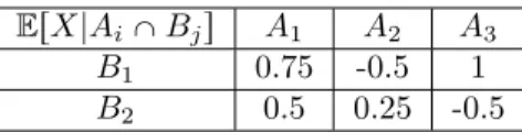
example one takes N0“ 2, Ap2q“ tA1, A2, A3u, B “ tB1, B2u and one generates
normal random values Xi with fixed variances σ2 “ 0.1 and such that the
probabilities and conditional expectations are given by the following table: P pAiX Bjq A1 A2 A3
B1 0.2 0.25 0.1
B2 0.25 0.1 0.1
ErX|AiX Bjs A1 A2 A3
B1 0.75 -0.5 1
B2 0.5 0.25 -0.5
Table 2: Conditional expectations of the generated random variables In particular,
P rAs “ pP pA1q, P pA2q, P pA3qq “ p0.45, 0.35, 0.2q,
P rBs “ pP pB1q, P pB2qq “ p0.55, 0.45q,
P pXq “ ErXs “ 0.225,
ErX|As “ pErX|A1s, ErX|A2s, ErX|A3sq » p0.611, ´0.286, 0.25q,
ErX|Bs “ pErX|B1s, ErX|B2sq » p0.227, 0.222q.
We generate n “ 10 values and we obtain the following data Xi A B 0.953 1 1 0.975 1 1 0.058 1 1 -0.766 2 1 -0.644 2 1 -0.819 2 1 0.028 2 2 0.627 2 2 1.04 3 1 -0.904 3 2
Table 3: Generated random variables
In this case, the usual mean is the sum of all Xi over 10 that is we assign the
weight 1{n “ 0.1 at each Xi and we have PnpXq » 0.055. When we rake one
time we assign the weights 0.15, 0.07, 0.1 at individuals belonging respectively to A1, A2, A3. The raked mean for N “ 1 is
Pp1qn pXq “ 0.15 ˆ P pA1q PnpA1q ` 0.07 ˆ P pA2q PnpA2q ` 0.1 ˆ P pA3q PnpA3q » 0.2. When the algorithm is stabilized in this case the final weights are given by the following table:
wip8q A1 A2 A3
B1 0.15 0.024 0.029
B2 X 0.139 0.17
Table 4: Final raked weights
Notice that the cross means that we do not generate random variables belonging to A1X B2 due to a low value of n. The final raked mean is Pp8qn pXq » 0.212
B
Calculation of σ
fp8qWe use the notations of the section 4.4 of [1] concerning the proof of their Proposition 11 in the aim to establish the expression of Gp8q. The calculation
uses the two following stochastic matrices
PA|B“ˆ P pA|Bq P pA C |Bq P pA|BCq P pAC|BCq ˙ “ ˆ pAB{pB 1 ´ pAB{pB ppA´ pABq{pB 1 ´ ppA´ pABq{pB ˙ , PB|A“ˆ P pB|Aq P pB C |Aq P pB|ACq P pBC|ACq ˙ “ ˆ pAB{pA 1 ´ pAB{pA ppB´ pABq{pA 1 ´ ppB´ pABq{pA ˙ , (B.1) the two following conditional expectation vectors
Erf |As “ pErf |As, Erf |ACsq, Erf |Bs “ pErf |Bs, Erf |BCsq, (B.2) the two following covariance matrices
VarpGrAsq “ pApA ˆ 1 ´1 ´1 1 ˙ , VarpGrBsq “ pBpB ˆ 1 ´1 ´1 1 ˙ . (B.3)
and the two following vectors V1pf q “ Erf |As ´ PB|A¨ Erf |Bs
“ ˆ Erf |As Erf |ACs ˙ ´ ˆ pAB{pA 1 ´ pAB{pA ppB´ pABq{pA 1 ´ ppB´ pABq{pA ˙ ¨ ˆ Erf |Bs Erf |BCs ˙
“ pErf sppA´ pABq ´ Erf |AspApB` Erf |BsppAB´ pApBqq ¨
ˆ
´1{pApB
1{pApB
˙ ,
V2pf q “ Erf |Bs ´ PA|B¨ Erf |As
“ ˆ Erf |Bs Erf |BCs ˙ ´ ˆ pAB{pB 1 ´ pAB{pB ppA´ pABq{pB 1 ´ ppA´ pABq{pB ˙ ¨ ˆ Erf |As Erf |ACs ˙
“ pErf sppB´ pABq ´ Erf |BspApB` Erf |AsppAB´ pApBqq ¨
ˆ
´1{pApB
1{pApB
˙ .
The eigenvalues of PA|B¨ PB|A and PB|A¨ PA|B are 1 and T1“ T2 “ ppAB´
pApBq2{pApApBpB. Their eigenvectors associated to T1and T2are respectively
ppB{pB, ´1qtand ppA{pA, ´1qtwhich implies
U1“ ˆ1 pA{pA 1 ´1 ˙ , U2“ ˆ1 pB{pB 1 ´1 ˙ .
For the case of two marginals, Albertus and Berthet showed that GpN qconverge
almost surely to Gp8q
pf q “ Gpf q ´ S1,evenpf qt¨ GrAs ´ S2,oddpf qt¨ GrBs where
S1,evenpf q “ U1 ˆ0 0 0 p1 ´ T1q´1 ˙ ¨ U1´1¨ V1pf q “ C1,evenpf q ˆ ´pApB pApB ˙ , C1,evenpf q “ Erf |Bspp
AB´ pApBq ´ Erf |AspApB´ Erf sppAB´ pAq
pApBpApB´ ppAB´ pApBq2 , S2,oddpf q “ U2 ˆ0 0 0 p1 ´ T2q´1 ˙ ¨ U2´1¨ V2pf q “ C2,oddpf q ˆ ´pApB pApB ˙ ,
C2,oddpf q “ Erf |Aspp
AB´ pApBq ´ Erf |BspApB´ Erf sppAB´ pBq
pApBpApB´ ppAB´ pApBq2
.
By linearity of f ÞÑ Gpf q and the fact that Gpaq “ 0 for any constant a P R one can write
Gp8qpf q “ G pf ` pBC1,evenpf q1A` pAC2,oddpf q1Bq ,
which implies that
σp8qf “ VarpGp8q
pf qq
“ Varpf q ` VarppBC1,evenpf q1A` pAC2,oddpf q1Bq
` 2Covpf, pBC1,evenpf q1A` pAC2,oddpf q1Bq
“ Varpf q ` pApAp2BC 2 1,evenpf q ` p 2 ApBpBC2,odd2 pf q ` 2pApBC1,evenpf qC2,oddpf qppAB´ pApBq ` 2pApBpC1,evenpf q∆A` C2,oddpf q∆Bq
With some calculations we find the simple expression of σp8qf given by (2.11).
References
[1] Albertus, M. and Berthet, P. (2019). Auxiliary information: the raking-ratio empirical process. Electron. J. Stat., 13(1):120–165.
[2] Bankier, M. D. (1986). Estimators based on several stratified samples with applications to multiple frame surveys. Journal of the American Statistical Association, 81(396):1074–1079.
[3] Berthet, P. and Mason, D. M. (2006). Revisiting two strong approximation results of Dudley and Philipp. 51:155–172.
[4] Binder, D. A. and Th´eberge, A. (1988). Estimating the variance of raking-ratio estimators. Canad. J. Statist., 16(suppl.):47–55.
[5] Brackstone, G. J. and Rao, J. N. K. (1979). An investigation of raking ratio estimators. The Indian journal of Statistics, Vol. 41:97–114.
[6] Choudhry, G. and Lee, H. (1987). Variance estimation for the canadian labour force survey. Survey Methodology, 13(2):147–161.
[7] Deming, W. E. and Stephan, F. F. (1940). On a least squares adjustment of a sampled frequency table when the expected marginal totals are known. Ann. Math. Statistics, 11:427–444.
[8] Ireland, C. T. and Kullback, S. (1968). Contingency tables with given marginals. Biometrika, 55:179–188.
[9] Konijn, H. S. (1981). Biases, variances and covariances of raking ratio esti-mators for marginal and cell totals and averages of observed characteristics. Metrika, 28(2):109–121.
[10] Sinkhorn, R. (1964). A relationship between arbitrary positive matrices and doubly stochastic matrices. Ann. Math. Statist., 35:876–879.
[11] Stephan, F. F. (1942). An iterative method of adjusting sample frequency tables when expected marginal totals are known. The Annals of Mathematical Statistics, 13(2):166–178.
[12] van der Vaart, A. W. and Wellner, J. A. (1996). Weak convergence and empirical processes. Springer Series in Statistics. Springer-Verlag, New York. With applications to statistics.