Acoustic tomography in the straits of Florida

ACOUSTIC TOMOGRAPHY IN THE STRAITS OF

FLORIDA

by

David Brian Chester

B.S. Southampton College of Long Island University (1986)

Submitted in partial fulfillment of the requirements for the degree of

Master of Science at the

MASSACHUSETTS INSTITUTE OF TECHNOLOGY and the

WOODS HOLE OCEANOGRAPHIC INSTITUTION September 1989

© David B. Chester 1989

The author hereby grants to MIT and to WHOI permission to reproduce and to distribute copies of this thesis document in whole or in part.

Signature of Author ... ... ...

Joint Program in Physical Oceanography Massachusetts Institute of Technology Woods Hole Oceanographic Institution July 26, 1989

Certified by ...--. . ... . ... Paola Malanotte-Rizzoli Associate Professor of Physical Oceanography

ST esis Supervisor

Accepted by... ... .... ... 4...

-. Carl Wunsch

rman, Joint Committee for Physical Oceanography I TUE Massachusetts Institute of Technology

L 1Woods Hole Oceanographic Institution

NOVL

'

ACOUSTIC TOMOGRAPHY IN THE STRAITS OF FLORIDA by

David Brian Chester

Submitted in partial fulfillment of the requirements for the degree of Master of Science at the Massachusetts Institute of Technology

and the Woods Hole Oceanographic Institution July 27, 1989

Abstract

Variability of the Florida Current has been monitored via acoustic tomography. A reciprocal tomography experiment was conducted in the eastern half of the Florida Straits during mid October and November, 1983. A triangular array of transceivers, with leg separations of approximately 45 kilometers, was deployed at 270_{N. The}

presence of a surface mixed layer in the region allowed for the ducted propagation of acoustic energy in the surface layer. A deeper layer was sampled by an unresolved group of refracted, bottom reflected ray arrivals. Incorporating the complete set of arrivals, we are able to obtain depth dependent estimates of the temperature field, current velocity, and relative vorticity. The oceanography of the region has been shown to be dominated by the lateral shifting of the surface and subsurface core of the Florida Current. The influx of westward flowing water through the North-west Providence Channel at 260_{N also appears as a large scale signal in the eastern}

Florida Straits. Low frequency fluctuations of temperature, current velocity, and vorticity occur at periods ranging from several days to nearly two weeks, and are intimately related to meandering of the Florida Current system.

Thesis Supervisor:

Dr. Paola Malanotte-Rizzoli, Associate Professor Massachusetts Institute of Technology

Contents

2 The Florida Straits Tomography Experiment 10 2.1 Oceanography of the Region ... .. 10

2.2 Experimental Design .... . . ... ... 15

2.3 Environmental Data ... 19

2.4 The Processed Data ... 24

3 Ocean Acoustics and the Forward Problem 33 3.1 Ray Theory ... ... 33

3.2 Ray Arrivals in Shallow Water ... 39

3.3 Formulation of the Forward Problem . ... 54

4 The Inverse Problem 59 4.1 Formulation of the Inverse Problem . ... 59

4.2 The Singular Value Decomposition . ... 63

4.3 Resolution and Variance ... 70

5 Oceanographic Variables 75 5.1 Tem perature ... ... 75

5.2 Current Velocity ... 80

5.3 Vorticity ... ... . ... 84

5.4 Discussion and Conclusions ... .... 87

Acknowledgments

First and foremost, I would like to thank my thesis advisor, Paola Malanotte-Rizzoli, for the continual guidance, enthusiasm, encouragement, and freedom she has given me along the way. The acoustic data set was graciously provided by Harry DeFerrari and his group at the University of Miami, RSMAS. The STACS current meter mooring data was provided by Rainer Zantopp, Friedrich Schott, and Tom Lee, also from the University of Miama, RSMAS. Numerous people have aided me in the development of this thesis, but I would especially like to thank Carl Wunsch, Jim Lynch, Harry DeFerrari, Dong-Shan Ko, and Bill Johns for stimulating discussions concerning various aspects of the thesis, and oceanography in general. Thanks also go to Anne-Marie Michael for assistance in the preparation of the manuscript.

Chapter 1

Introduction

1.1

Historical Backgound

The Florida Current plays a major role in the North Atlantic heat budget by transporting mass and warm water poleward through the Straits of Florida. The bathymetry of the Florida Straits, with Florida to the west and the Bahama Banks to the east, constrains the Florida Current to be a narrow, yet intense western boundary current. Upon exiting the Straits, the Florida Current evolves into a larger and more diffuse current as it connects with the Gulf Stream.

The study of the Florida Current is now over a century old. In a remarkable endeavor, Pillsbury (1891) directly measured currents to depths of 250 meters at various stations across the Straits and observed high frequency (tidal) oscillations of the flow, as well as lateral shifting of the Florida Current core. Volume transports of the Florida Current were calculated by Wiist (1924) and Parr (1937) using the dynamic height method. Montgomery (1938) and Hela (1952) noted seasonal fluc-tuations in the strength of the the Florida Current by observing sea level changes at tidal stations in the Straits. Large amplitude tidal and seasonal variations of the Florida Current mass transport were also obtained by Wertheim (1954) using the electropotential method with an underwater telegraph cable connecting Key West, Florida and Havana, Cuba.

Our understanding of the dynamics of the Florida Current has increased dra-matically in the last twenty-five years as oceanographic instrumentation has evolved. Transport float measurements (Richardson and Schmitz, 1965; Schmitz, 1969; and Richardson et al., 1969) have given us a much clearer picture of the velocity struc-ture of the Florida Current. Wunsch et al., (1969) used spectral analysis of tide gauge records to infer time scales of variability of the Florida Current. Nontidal fluc-tuations in the Florida Straits, with periods of several days to several weeks, have been related to atmospheric forcing by several authors (Diiing et al., 1979; Wunsch and Wimbush, 1977; and Lee and Mayer, 1977). Mean kinetic and potential en-ergy, as well as perturbation values, have been estimated across the Florida Straits (Brooks and Niiler, 1977). And most recently, the Subtropical Atlantic Climate Study (STACS) experiment was established to monitor long period fluctuations of mass and heat transport through the Florida Straits. Moored subsurface current meter arrays and the acoustic current profiler, along with tide gauges and a sub-marine cable, are the principal tools of measurement. Numerous papers concerning the spatial structure and temporal variability of the Florida Current have followed, including Molinari et al., 1985a,b; Lee et al., 1985; Leaman et al., 1987; Johns and Schott, 1987; and Schott et al., 1988.

Another technique for monitoring the activity of the Florida Current is acous-tic tomography. Ocean acousacous-tic tomography is a relatively new and promising method for determining oceanic structure and variability through the inversion of acoustic travel times to determine perturbations in sound speed (and hence tem-perature, density, and velocity). The idea was proposed by Munk and Wunsch (1979; 1982) as a practical tool for monitoring mesoscale fluctuations of an ocean basin. Several experiments have demonstrated the effectiveness of acoustic tomog-raphy in the mid ocean region (The Ocean Tomogtomog-raphy Group, 1982; Cornuelle, 1983; Cornuelle et al., 1985; Howe et al., 1987). Until recently, it was not clear that tomography would be a viable approach in a shallow, range dependent region

such as the Florida Straits. Unlike the open ocean, where the SOFAR channel acts a natural waveguide in refracting acoustic rays towards its axis, the sound speed structure in the Straits is such that all rays are refracted downward and forced to bounce off the seabed. Palmer et al., (1985), using a specialized acoustic ray tracing program, found that the identification of individual ray paths in the Straits is nearly impossible due to uncertainties in bathymetry.

Ocean acoustic propagation in the Straits of Florida was first studied nearly twenty-five years ago during the MIMI experiments (Steinberg and Birdsall, 1966). The phase variations of a 420 Hz continuous wave signal transmitted across the Florida Current compared favorably with changes of transport and temperature (Steinberg et al., 1972). More recently, a tomography experiment was set up in the Florida Straits with the objective of determining the feasibility of measuring variability in the Straits via acoustic methods (DeFerrari and Nguyen, 1986). Two three-point reciprocal transmission experiments were conducted at 270_{N in 1983.}

A small triangle, with leg separations of approximately 25 km, was situated on the western slope of the Straits. Results from this experiment can be found in DeFerrari and Nguyen, 1986; Ko, 1987; Monjo, 1987; and Ko et al., (1989). A larger triangular array, with leg separations of 45 km, was located on the eastern slope of the Florida Straits. This thesis will analyze the 40 day data set generated from the large triangle reciprocal tomography experiment of October, 1983.

1.2

Thesis Overview

The purpose of this thesis is to demonstrate the practicality of acoustic tomography as a monitoring scheme for a shallow water environment, specifically the Florida Straits. In so doing, it will be shown that accurate and reliable estimates of temperature, current velocity, and vorticity can be obtained quite readily. An

important result deriving from this thesis is the depth dependent estimation of the oceanographic variables.

The thesis is divided into five chapters. The 1983 Florida Straits tomography experiment is the subject of Chapter 2. To put the experiment in perspective, an overview of the hydrography of the Florida Straits region is given. A discussion of the experiment follows, along with the concurrent data from the STACS program. Finally, the processed acoustic data set is presented.

Chapter 3 introduces the forward problem of modelling acoustic propagation. Ray theory, based on Snell's law of refraction and the WKB approximation of a slowly varying medium with respect to acoustic wavelength, is chosen for the task. The principles of ray theory, and its application to a shallow water waveguide, are developed. The formulation of the forward problem then follows naturally.

The inverse problem is discussed in Chapter 4. The scheme of ocean acoustic tomography relies heavily on the machinery developed in the context of (geophys-ical) inverse theory. After formulating the inverse problem, a simple yet powerful solution technique is introduced, namely the singular value decomposition. The sin-gular value decomposition provides an insightful link between the forward modelling and the acoustic data. A residual benefit of the decomposition is the estimation of model and data resolution and variance, and this topic will be considered in some detail.

Chapter 5 discusses the results obtained from the 1983 acoustic tomography experiment. Inversion estimates of temperature, along with estimates of current ve-locity and vorticity are presented, and comparisons are made with the more conven-tional oceanographic measurements. A thorough description of the time dependent oceanographic field is then given. Finally, the results obtained from the analysis are summarized.

Chapter 2

The Florida Straits Tomography Experiment

2.1

Oceanography of the Region

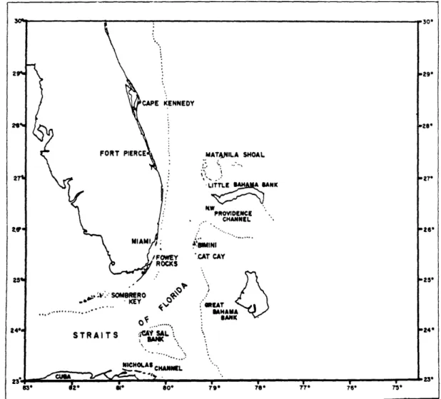
Before proceeding to a description of the oceanography of the Florida Cur-rent, the geographical setting is given. Figure 2.1 shows an overview of the region of study. The northern Straits of Florida (defined in this paper as extending from the tip of the Florida peninsula to the northern extent of the Little Bahama Bank) are the focus of this discussion. The coastline of Florida is the western boundary and the Bahama Banks are the eastern edge of the channel. The eastern bound-ary is not solid as the Northwest Providence Channel, reaching to a depth of 700 meters, divides the Great and Little Bahama Banks at latitude 260_{N. A vertical}

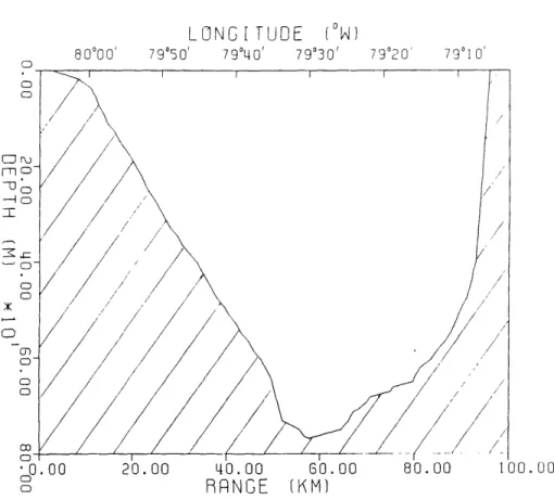
slice through latitude 270_{N is illustrated in Figure 2.2 to demonstrate the irregular}

bottom topography of the region. The seabed consists of a limestone (carbonate) base, with a surface layer of sediment a few meters thick (Malloy and Hurley, 1970).

The physical oceanography of the Straits of Florida is dominated by the Florida Current and its variability. The Florida Current is a northward flowing jet of warm water, with maximum surface velocities of 5 knots (2.5 m/s). The mass transport across the northern Straits is 30 ± 5 x 10 6 m 3/s, with an associated heat flux of 1-2 x 1015 watts. Despite the lateral constraints of the Florida peninsula and the Bahama Banks, meandering of the Florida Current is a commonplace occurence.

Meandering events typically extend several tens of kilometers in the lateral direction and hundreds of kilometers in the along-stream direction. The temporal variability of the Florida Current is a complex amalgamation of time scales, with equally energetic perturbations occurring with tidal, weekly, and seasonal periodicities.

Figure 2.1. An overview of the Florida Straits region, (adapted from Richardson et al., 1969). The dotted line represents the 100 fathom contour.

0.00 40.00 60.00 80.00

LONG[TUDE (0W)

80,000 79050' 79040' 79030/ 79020, 79010'

. .0 0 20.00 40.00 60

o RANGE (KM)

Figure 2.2. The bathymetry of the Florida Straits at 27*N. Vertical exaggeration is 1.0 x 102 in the lower graph. The upper graph shows a one to one scale of the bottom profile.

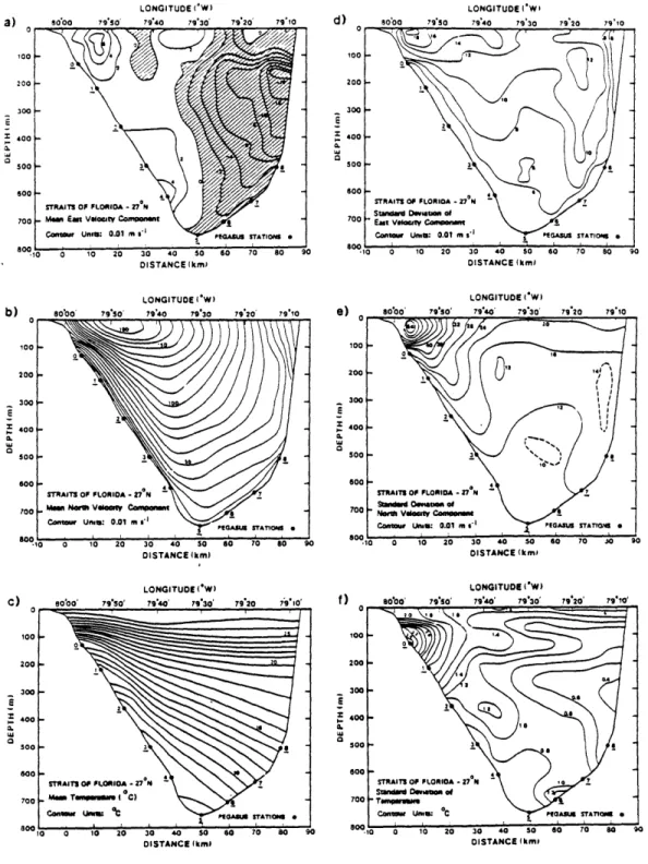
An 'average' picture of the Florida Current at latitude 270N, as seen by the Pegasus acoustic current profiler, is illustrated in Figure 2.3 (from Leaman et al., 1987). Figures 2.3a-c show cross sections of average east and north current velocity components and temperature, respectively, and Figures 2.3d-f show the associated standard deviations. Several important features should be pointed out. The core of the maximum surface velocities is displaced toward the western continental slope of Florida. In addition, the core of the current gradually shifts offshore with depth.

0.00

100.00

I i

A highly baroclinic structure is evident as the current speed decreases rapidly with depth. Looking at the horizontal shear (which is dominated by ~ as v >> u), a strong cyclonic shear zone is seen on the onshore side of the current and an anticyclonic region exists on the offshore edge. Also noteworthy is a large scale westward flow encroaching from the Northwest Providence Channel. Finally, the downward sloping of the isotherms from west to east is consistent with a geostrophic northward flow.

As previously mentioned, fluctuations of current velocities and temperature in the 2 to 20 day frequency band is dominated by energy associated with Florida Current meanders. Johns and Schott (1987) find that the most coherent, energetic meandering events occur at periods near 5 and 12 days. The downstream propa-gation of the 5 day (12 day) meander is found to have a phase speed of 36 km/d (28 km/d) and a wavelength of 170 km (340 km). The passage of meanders leads to a 'sloshing' of the thermocline, with upwelling and downwelling of isopycnals rearranging the cross stream structure of the current (Johns, personal communica-tion). Several mechanisms have been proposed for the generation of meanders in the Florida Current, such as shelf waves and barotropic and baroclinic instability in the presence of topography. The interaction of the Florida Current with the local topography of the Great Bahama Bank and Little Bahama Bank has been suggested as a source for larger scale variability in the Straits (Leaman and Molinari, 1987). Brooks (1975) proposes that a fluctuating wind stress can induce cross shelf pertur-bations via upwelling or downwelling associated with the Ekman transport being offshore or onshore. The jury is still out as to whether or not variations in local wind stress and wind stress curl are a primary source of energy for the meandering.

LONGITUDE I(W) a) 8000 7950' 79 40 79'30' 7920' 79,10 DISTANCE (km) LONGITUDE I'W) E 400 500 ooSoo 600 700 800 LONGITUDE I'W d) _ 0so'o 7950 7940) 79'30 DISTANCE (km) LONGITUDE ('W) DISTANCE (km) DISTANCE (km)

LONGITUDE ('W) LONGITUDE i'W)

DISTANCE Ikmi DISTANCE (km

Figure 2.3. The ensemble average (a-c) and standard deviation (d-f) of east and north velocity components and temperature, respectively, based on results of 16 Pe-gasus cruises to the Florida Current at 270N, (adapted from Leaman et al., 1987).

2.2

Experimental Design

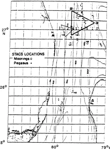
The October 1983 acoustic tomography experiment consisted of a triangular array of transceivers (with units acting as both sources and receivers) situated at 270_{N in the eastern half of the Florida Straits (see Figure 2.4). Transceivers 1}

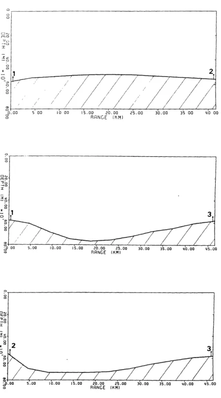
(26056'N, 79041'W) and 2 (27'19'N, 79041'W) are aligned nearly longitudinally, with transceiver 3 (27007'N, 79016'W) located just to the west of Little Bahama Bank. All three instruments were moored at a depth of 38 meters above the bottom. The distances between units 1-2, 1-3, and 2-3 are 41.5 km, 46.5 km, and 46.4 km, respectively. Figure 2.5 shows the bathymetry along the three legs of the triangle. Note that the leg connecting transceivers 1 and 2 is aligned almost parallel with the axis of the Florida Current, and the corresponding bottom topography is relatively flat. On the other hand, transmission from units 1 and 2 to 3, and vice versa, occurs over a steep and irregular bottom on the anticyclonic side of the Straits.

The resolvability of individual acoustic multipaths is a necessity in ocean acoustic tomography, and specialized signals have been developed for this task. The present day standard signal consists of a coded sequence of digits which exhibits pulselike characteristics upon reception and cross replication. Design of the signal involves several important tradeoffs which warrant a brief discussion. A high signal to noise ratio requires a powerful source. Identification of pulse arrival times requires a narrow pulse, and therefore a transmitted signal with a large bandwidth. But the transmission of a high power wide-band pulse is highly constrained by the limited power supply (batteries). Due to this limitation, transmissions are not continuous, but rather occur at regular intervals during most tomographic experiments. The typical multipath arrival signal is not an evenly spaced sequence of nonoverlapping delta functions. Instead, oceanic inhomogeneieties (such as internal wave

fluctua-tions) lead to constructive and destructive interference of multipaths, and a blurred envelope of arrivals which varies with time results. To overcome this problem, periodic pulses are transmitted and coherently averaged at the receiver to boost the signal to noise ratio. The maximum number of pulse repetitions is limited by the ocean coherence time, which is generally considered to be several minutes. For more details of the signal design and processing for tomography, the reader is referred to excellent discussions given by Spindel (1985) and Metzger (1983).

270 N

260

250

800 790W

Figure 2.4. Location of the October 1983 tomography array (large triangle), (adapted from DeFerrari and Nguyen, 1986). Also shown is the location of the August 1983 tomography array (small triangle), along with STACS 4 moorings 146-149, and Pegasus stations 0-8.

Figure 2.5. Bottom topography along the three legs of the tomographic array. The transceivers are moored 38 meters above the bottom.

Getting back to the 1983 tomography experiment, the transmitted signal consisted of a frequency modulated linear maximal pseudorandom sequence. The carrier frequency was 459.5588 Hz, with a bandwidth of 100 Hz. The source level was approximately 176 db re 1 pPa at Im. The repetition period of the transmitted signal (2.2 s) was greater than the total spread of multipath arrivals (1.5 s), so no overlapping of arrivals occurred. A summary of the signal parameters for the 1983 large triangle experiment is given in Table 1.

Table 1: Signal Parameters for the October 1983 Florida Straits Experiment

Carrier frequency 459.5588 Hz Bandwidth 100 Hz Digits 255 Digit duration 0.0087 s Sequence duration 2.2195 s Repetitions 135 (4.99 min)

The transmission schedule commenced (time 0) with unit 1 transmitting (for approximately 5 minutes) to units 2 and 3, which received and processed the signal. Approximately 2 minutes after the first transmission (or 7 minutes from time 0), unit 2 transmits to units 1 and 3. The two minute wait is necessary to allow for propagation of the signal (which takes nearly 30 seconds) and processing of the received signal. Approximately 2 minutes later (or 14 minutes from time 0) unit 3 transmits to units 1 and 2. The entire 'sing around' time takes about 20 minutes. The instruments then wait until the beginning of the next hour (approximately 40 minute wait period) to repeat the cycle.

The received signals were first bandpass filtered, amplified, then sampled at four times the carrier frequency. The next step was complex demodulation (a pulse compressing summation process). The resulting demodulates were then coherently averaged with subsequent sequences (over the full 5 minute period), yielding a record of 510 complex demodulate pairs. The demodulate pairs were then stored internally on a cassette tape. Correlation with a replica of the transmitted linear maximal pseudorandom sequence was not done in situ.

The October 1983 acoustic tomography experiment generated a complete 40 day data set of reciprocal hourly transmissions for all three instruments.

2.3

Environmental Data

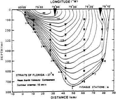
We are fortunate that the October 1983 tomography experiment occurred simultaneously with the STACS program. A subsurface moored array of Niskin Wing and Aandera current meters was maintained across the Florida Straits for several years (see Figure 2.4 for the location of the STACS 4 moorings). Direct measurements of current velocities and temperature at several depths were recorded. A sawtooth array was deployed in hopes of studying meandering variability and propagation. A vertical slice through 270_{N is pictured in Figure 2.6, showing the}

spatial coverage of the STACS 4 array. Note that no current meters extend to the high velocity core (upper 150 meters) of the Florida Current. In addition to the current meter data, Pegasus acoustic profiles of temperature and horizontal velocity were obtained at regular intervals at eight station across the Straits (see Figure 2.4 and 2.6 for locations of the Pegasus stations). The Pegasus data set is valuable because it gives us measurements over the entire water column, including the surface layer which is not sampled by the current meter array.

LONGITUDE 4(W)

DISTANCE (km)

Figure 2.6. Moored current meter coverage superimposed on mean downstream velocity contours from Pegasus sections, (adapted from Leaman et al., 1987). The location of the Pegasus sections (0-8) are marked at the bottom. The triangles at the surface indicate the lateral extent of leg 1-2 and vertex 3 of the October 1983 tomography array.

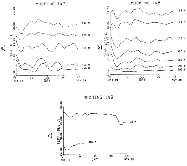
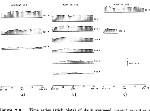
Time series of velocity and temperature from the current meters are discussed first. Temperature time series (Figures 2.7a-c) and velocity time series (Figures 2.8a-c) are presented for moorings 147, 148, and 149 from the middle of October until the end of November. The temperature and velocity records have been 3 hour bandpass filtered, sampled at hourly intervals, then daily averaged. Mooring 147 is closely aligned with the 1-2 leg of our tomographic array, but displaced 20 km upstream. Time series from mooring 147 sample the eastern edge of the current core. Mooring 148 is located close to the lower leg of the tomographic array and captures much of the energetic variability of the current. Mooring 149 contains an incomplete record (with only one current meter yielding a full time series) of the eastern region.

MOORING 1417 MOORING 148 142 M 189 M 301 M 402 446 h 10 20 30 40

OCT 19 OAT NOV 28

_,o IC) b) LU3_C3 M M OCT 19 MOORING 149 Un .95 M L3 C 0 a M. 0 300 K -0 10 2b 30 40

OCT 19 OAT NOV 28

Figure 2.7. Time series of daily averaged temperature at each current meter for (a)mooring 147, (b)mooring 148, and (c)mooring 149. Day 0, the beginning of the experiment, corresponds to October 19.

We now turn to the Pegasus acoustic velocity profiler data set. A summary of Pegasus observations in the Florida Straits can be found in a report by Vertes and Leaman (1984). The Pegasus profiler is an acoustically tracked, free-falling instru-ment which gives continuous measureinstru-ments of horizontal velocities and tempera-ture (see Spain et al., (1983) for a complete discussion of the velocity profiler).

C3 CD ,,o_I, I0CD U a)

C3

\rJV"?

MOORING j147 MOORING 148 MOORING 119

N

trrrTTtt Htf TITTfITTTtTTTItTU Ttrttf 59I I 10 1S M

692 n

O i b 20 I jb 3b 3' Mb o1 30 4b b 3 4

OCT 19 ORT NOV 28 OCT 19 DAT NOv 28 OCT 19 OAT NOV 28

a) b) c)

Figure 2.8. Time series (stick plots) of daily averaged current velocities at (a)mooring 147, (b)mooring 148, and (c)mooring 149. Day 0, the beginning of the experiment, corresponds to October 19.

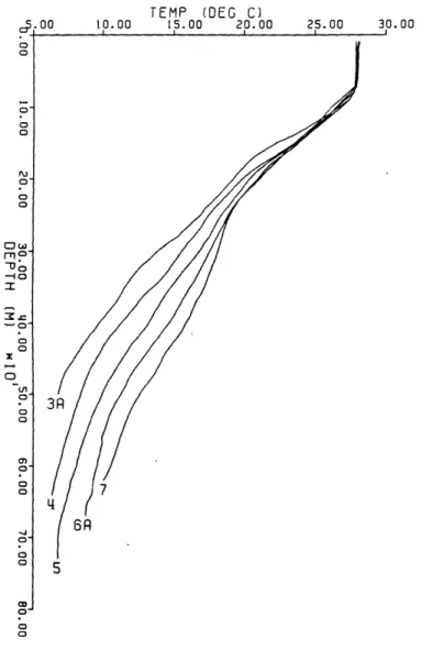
Temperature profiles for stations 3a-7, averaged over five up/down casts and a several day period (October 28 - November 4) are presented in Figure 2.9. Note that station 3a is directly in line with the path connecting the north/south leg of the tomographic array.

A good picture of the oceanographic setting can be obtained from these two data sets. From the Pegasus data set, a nearly isothermal mixed layer extending to a depth of 100 meters is evident at all stations. Beneath the mixed layer the temperature decreases steadily with depth, with warmer water penetrating to greater depths as the Bahama Bank is approached. Typical current velocities at the

quite coherent with depth. The mooring records show an energetic meandering event at the outset which is readily detected by the large drop in current velocity at mooring 147. Several smaller scale events, with periodicities near two weeks, are suggested by the temperature and velocity fluctuations. A detailed discussion of the oceanography will be presented in comparison with the inverse results in Chapter 5.

TEMP (DEG C)

10.00 15.00 20.00 25.00 30.00

Figure 2.9. Average temperature profiles for late October - early November at Pegasus stations 3a-7.

23 5.00 o 0 R-0* 00_o ru0 Ow --Do0 I "o 0 0 Ln 0U, o_0" 0 |I I Ii

2.4

The Processed Data

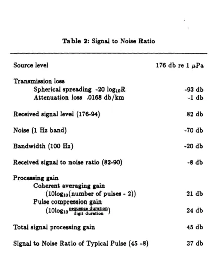
The received signal was first cross correlated with a replica of the transniutted signal. The result of this operation was a pulse response of 510 complex samples with a sampling interval of 4.352 ms (2.2195 s / 510 samples). This procedure was applied to all six records. Hereafter we will refer to the data records as S1R2 (signifying transmission from source 1 to receiver 2), S2R1, S1R3, S2R3, S3R1, and S3R2. The signal to noise ratio of an average pulse response was about 35 db (Table 2). It is not necessary to know the exact intensity of the pulse response as the inversion scheme used in this thesis is based on the travel time arrival of pulses.

Table 2: Signal to Noise Ratio

Source level Transmission loss

Spherical spreading -20 logoR Attenuation loss .0168 db/km Received signal level (176-94)

Noise (1 Hz band) Bandwidth (100 Hz)

Received signal to noise ratio (82-90) Processing gain

Coherent averaging gain

(10log1o(number of pulses - 2))

Pulse compression gain

(10lo-to guen. du"mtion (l10odiggt duration) Total signal processing gain

Signal to Noise Ratio of Typical Pulse (45 -8)

176 db re 1 uPa -93 db -1 db 82 db -70 db -20 db -8 db 21 db 24 db 45 db 37 db

A typical pair of reciprocal hourly pulse responses of S1R2 and S2R1 is plot-ted in Figures 2.10a,b. Relative travel time is plotplot-ted along the abscissa, with time zero corresponding to the first of the 510 samples. Absolute travel time is not used for the acoustic record because of navigational inaccuracies in the determination of the source/receiver separation distance, and hence pulse arrival time. The ordinate represents signal to noise ratio, in db, for the first hourly pulse response.

Consec-S1R2

S2R1

.oo 0 0.50so 1'.00 1.50 2.00 .00 0.50 1.00 1.50 2.00

TRAVEL TIME (S) TRAVEL TIME (S)

a) _b)

Figure 2.10. Reciprocal hourly pulse responses of (a)S1R2 and (b)S2R1 for a typical day (day 5 in this case). Relative travel time is plotted along the abscissa, with the ordinate representing the signal to noise ratio (or acoustic intensity).

utive hourly transmissions are then offset by a constant amount to aid in viewing. Looking closely at Figures 2.10a,b we see that identification of individual multipaths is not a simple task. The appearance and disappearance of multipaths is attributed to the influence of tides and internal waves. It is also evident that the hourly pulse responses from reciprocal transmissions are not identical.

A much clearer picture evolves when we take the daily average of 24 hourly pulse responses. By doing this we avoid aliasing of the dominant tidal and internal wave signals while simultaneously decreasing the random noise level. The six data records of daily averaged pulse responses, normalized by the daily averaged noise, are shown in Figures 2.11a-f. Several features are prominent in all of the plots. The most obvious signal is a large peak which is seen as the latest arrival in all records. This peak always exists, although the shape (multipath structure) varies from day to day. It will later be shown that this peak corresponds to a path of propagation which samples the lower 300 meters of the water column. The precursor arrivals, most evident in the pulse responses of S1R2 and S2R1, correspond to paths of propagation which are surface ducted. These early arrivals did not exist in the August 1983 experiment (Ko, 1987). Their appearance is due to the surface mixed layer which acts to trap rays. The pulse responses of daily averaged reciprocal transmissions are seen to be quite similar, with small scale differences still obvious. A further discussion of the pulse responses is given in Section 3.2 in conjunction with the ray theoretical arrival predictions.

Another issue to be discussed at this time is the identification of the processed pulse arrival times, and errors associated with this identification. Arrival times were estimated by taking the center of mass of the most intense peaks in the pulse response record. A minimum threshold was set, and only those peak samples which exceeded this limit were used in the estimate. The arrivals for S1R2 and S2R1 (except for day 10 where the noisy reception is not understood) are stable with

a) b)

Figure 2.11. Daily averaged pulse responses for (a)S1R2, (b)S2R1, (c)S1R3, (d)S3R1, (e)S2R3, and (f)S3R2

S1.R3 0 _S3

_I

co

CC: OD

. co

RAVL I ME S) RAVL TME 3) .0

)d)

time and easily identified. A very small percentage of the processed data (less than 5 percent) had to be edited to remove high ambient noise levels. Also, if a pulse could not be identified above the background noise, the travel time was interpolated from the previous and later corresponding arrivals. The same procedure was applied to the pulse responses of S1R3, S3R1, S2R3, and S3R2. The precursor pulse arrivals for these four records showed less stability, thereby complicating the identification process. More of the pulse response data (approximately 25 percent) needed editing. It should be noted that a gross misidentification of an arrival time will show up in the output of the inversion as an unrealistic oceanographic fluctuation. On the other hand a slight error in arrival time estimation may be falsely interpreted as an oceanographic signal which does not really exist. Applying an error to the measured data (pulse arrival time) in the inversion is used to mitigate this problem.

The precision of travel time resolution has significant implications. Temper-ature variations cause the largest fluctuations in pulse travel time. A temperTemper-ature deviation of 2"C corresponds to a change in travel time of about 200 ms (for a 45 km range). Current induced fluctuations in travel time are much smaller. A 50 cm/s current (acting over a 45 km range) will alter the travel time by only 10 ms. So an uncertainty of 5 cm/s in current velocity is the maximum precision attainable for a travel time error of 1 ms.

The estimation of travel time variance is not a simple task. The major source of error is insufficiently resolved rays which arise due to multipath interference. In-ternal wave related variance is the next most important random error, with errors in the signal processing being minimal. From the 1983 reciprocal tomography ex-periment (which was conducted near Bermuda), the internal wave induced variance was estimated to be about 10 ms' (see Stoughton et al., 1986). The transmission range for the 1983 reciprocal tomography experiment was 300 km, which is much longer than the 45 km range of the Florida Straits experiment. The internal wave

induced variance is directly related to the rms phase delay along the ray path, which is roughly proportional to range (see Flatte et al., 1979). We thus expect a smaller variance due to internal wave effects in the Florida Straits experiment due to the much shorter transmission range. DeFerrari and Nguyen (1986) were able to resolve tidal currents in the Florida Straits from the small triangle tomography experiment, and estimated the total rms travel time error for the experiment to be about 0.2 ms. The small triangle experiment had a transmission range of roughly 25 km, and a quicker transmission rate (a complete cycle of reciprocal transmissions took place every 12 minutes). Table 3 gives the estimated travel time variance for this experiment. The daily averaged travel time is estimated to have an rms error of about 1 ms.

Table 3: Travel Time Variance

Matched filter receiver precision (a, variance)

o, = [27r(6f),rm.,()j-1 0.07 ms' Interpolation error variance 0.05 ms2 Internal wave related variance 5 ms2 Interference related variance 10 ms2

Total variance 15 ms2

Daily mean variance - 1 ms2 Daily averaged rms travel time error - 1 ms

Errors arising from mooring motion and clock timing have not yet been addressed. The transceivers for this experiment were moored 38 meters above the bottom. If we assume a 1 m/s current acting on the entire mooring, a maximum horizontal displacement of 0.5 meters is estimated (DeFerrari and Nguyen, 1986).

This change in ray path length would correspond to a maximum travel time error of 0.3 ms. Clock drift is a nonreciprocal error which is due to a clock at one of the units being fast relative to a clock at another unit. Correcting clock timing errors is usually accomplished by a linear detrending of the clock drift referenced to a more precise standard clock. Unfortunately, the final clock readings were not obtained during this experiment. This does not present a problem in the estimation of temperature and vorticity as the clock errors cancel with reciprocal transmissions. But the clock error does not cancel in the estimation of the current. This issue will be discussed in Section 5.2 when we consider the estimation of current in more detail.

Chapter 3

Ocean Acoustics and the Forward Problem

3.1

Ray Theory

The forward problem of modelling acoustic propagation in an oceanic wave-guide can be attacked in several manners, all of which involve solving the wave equation. Perhaps the simplest and most physically insightful method is a de-velopment in terms of acoustic rays, which have a direct analogue in the field of optics. Implicit in the ray theoretical approach is the assumption that the refractive properties of the medium change only slightly over an acoustic wavelength (this is geometrical optics, or the WKB approximation). Snell's law of refraction is the re-sult of this formulation, and the paths of energy propagation through the medium are explicitly specified. But ray theory is not an exact solution for the acoustic wavefield, and as such does not account for diffraction and other wave effects. Nev-ertheless, ray theory was chosen for this analysis due to the simplicity of matching pulse arrival times with ray theoretical predictions and the ease of constructing the inverse operator (ray path spatial coverage).

Before proceeding, two other theoretical approaches to solving the wave equa-tion should be menequa-tioned. Normal mode theory gives an exact soluequa-tion to the wave equation based on the preferred vibrations (normal modes) of the waveguide. The normal mode picture becomes complicated when the medium is range dependent

(due to irregular bathymetry and/or strong inhomogeneities such as fronts or ed-dies), and mode coupling must be considered. A second approach, the parabolic equation method, is based on the paraxial (small angle) approximation to the wave equation. The result is a model which is very useful for modelling propagation in a range dependent waveguide.

A development of the solution to the wave equation in terms of rays is now given. We follow in similar fashion to a derivation found in Tolstoy and Clay (1966). Other good references include Officer (1958) and Brekhovskikh and Lysanov (1982). The wave equation is given by

V2 1 2p 0, (3.1)

c2 0t 2

where p is the acoustic pressure and c is the sound velocity, which may vary with the spatial coordinates (i.e., c = c(x, y, z)). For a harmonic source e- ' t, the wave equation becomes the Helmholtz equation

V2p + k2p = 0, (3.2)

with k being the wavenumber in the direction of propagation. We rewrite the wavenumber k as

w w co

k =kon , (3.3)

C Co C

where co is a constant reference sound velocity and n = 2 is the index of refraction.C Without loss of generality we represent the acoustic pressure as

where A is the wave amplitude and kS is the phase of the wave. Substituting (3.4) into (3.2), and collecting real and imaginary terms, we are left with two equations:

V2A - k2A [n2 _{- (VS)}2_{] = 0, (3.5)}

and

2VA - VS + AV 2S = 0. (3.6)

Up to this point the equations are exact solutions to the wave equation.

We now follow in the footsteps of ray optics and make the assumption

V2A

<< 1. (3.7)

k2A

A strict interpretation of this assumption is that the rate of variation of the wave phase (per wavelength) of the vertical component of wavelength is small (see Tolstoy and Clay (1966)). More generally, the fractional change in the sound speed gradient (d) must be small in comparison with the gradient {, where A is the acoustic_{dz A'} wavelength. Simpler yet, the propagating medium must vary only slightly over an acoustic wavelegth.

Applying this condition (Equation (3.7)) to Equation (3.5), we then have

(Vs)2 = n , (3.8)

or writing out the operator

( )2 + ( )2 + ( )2 = n . _(3.9)

This is the eikonal equation, and the cornerstone of ray theory. A physical picture of rays follows direcly from the solutions to the eikonal equation. Surfaces of constant phase (wave fronts) are given by S = constant, and the orthogonals to the wave fronts (VS) define the rays. The rays represent the paths along which acoustic energy is propagated. The amplitude of the rays is given by Equation (3.6), which is often referred to as the transport equation. It should be noted that the eikonal equation is not necessarily a solution to the wave equation due to the geometrical optics approximation.

We now wish to parameterize the acoustic rays in terms of the refractive properties of the medium. The formulation of the ray path equations follows directly from the eikonal equation, and is presented here for completeness. The unit vector along a ray (normal to an S = constant surface) is given by

n d = VS, (3.10)

ds

where r = r(x, y, z) and s is the arc length along the ray. Differentiating along a ray path (-), and using the eikonal equation and Equation (3.10), we obtain

d dr

S(n-)

= Vn. (3.11)

ds ds

This equation describes the ray trajectories in terms of the index of refraction n = _{n(x,y,z). Rewriting (3.11) in component form,}

d dx On d(n (3.12a) ds ds E ' d dy dn S(n ) a, (3.12b) ds ds ay

d dz On

-(n-)

ds ds az

These equations are often called the ray path equations, and are a generalization of Snell's law.

It should be noted that the ray paths satisfy Fermat's principle. The time of arrival of a ray is given by the integral

S= ds , (3.13)

where ds is arc length along the ray and r represents the ray path. Fermat's principle states that the travel time along a ray path is an extremum (i.e., 6r = 0). In real physical space a ray represents a path of stationary time, and the travel time is given by the minimum value. The ray path equations, along with Fermat's principle, allow us to trace rays through a medium varying in all three directions (i.e., c = c(x,y,z)).

For most practical cases of ray tracing, we consider propagation in the vertical plane with the sound speed a function of depth only (i.e., c = c(z)). This is a good approximation due to the vertically stratified nature of the oceanic waveguide. So if we consider propagation in the r - z plane, where r is horizontal range, our ray

path Equations (3.12) become

d dr On -(n-) -5 - 0 (3.14) ds ds Or d dz an dn =(n ) . (3.15) ds ds 4z dz

From Equation (3.14a) we see that

dr

n-

=

If we take 0 as the angle which the ray makes with the vertical, then d = sin 9, and we arrive at

sin 9

nsin9 = _c - p (constant). (3.17)

This is Snell's law, and can be considered a statement of the conservation of the horizontal component of the wavenumber along a ray path when c = c(z). It is a very useful relation as it allows us to trace the refraction (bending) of ray paths through a variably refracting medium. The ray parameter p is constant along a given ray path but varies from one ray to another. It is also useful to note that for the case of a constant sound speed gradient (linear c(z) profile), the rays trace out arcs of a circle.

Most ray tracing programs use constant sound speed gradient segments to approximate a continuous sound speed profile. Different sound speed profiles can be specified at various ranges for the range dependent case. Interpolation between successive locally range independent sound speed profiles gives the sound speed as a function of range. The ray paths are then calculated by integration of the ray path equations (as specified by Snell's law). The ray is assumed to travel in a vertical plane connecting the source and receiver. Out of plane effects which produce horizontal sound speed gradients are assumed to be small. The sound speed profiles are such that only a few ray paths actually connect a given source and receiver. These paths are called eigenrays. Ray tracing programs typically send out a fan of rays (with slightly offset launch angles), and march along in range in accordance with Snell's law to the range of the receiver. The eigenrays are then the paths which 'hit' the receiver.

Brief mention is now made of two of the problems encountered during ray tracing. Firstly, by dividing the sound speed profile into segments of constant sound speed gradient, we are left with discontinuities in L. These discontinuities may lead to a spurious focusing effect, often referred to as a false caustic. This problem may be alleviated by using curved line segments to approximate the velocity profile. Secondly, ray theory (geometric optics) is, in principle, a no reflection theory. Corrections need to be applied at caustics and turning points. This can be accomplished by keeping more terms in the WKB approximation.

In this analysis, we use the range dependent eigenray program MPP (multiple profile ray tracing program) developed by C. W. Spofford. The sound speed field is linearly interpolated in both depth and range in specified triangular sectors. The bottom bathymetry is represented by piecewise linear segments. Output of the program includes eigenray arrival times and transmission loss (calculated form geometrical spreading and losses due to boundary reflections), along with a history of the eigenray trajectories.

3.2

Ray Arrivals in Shallow Water

Acoustic propagation in the ocean is intimately related to the structure of the sound speed profile. Sound speed may be calculated with the simple equation (Medwin, 1975)

c = 1449.2 + 4.6T - 0.055T2 + 0.00029T3 _{+ (1.34 - 0.010T)(S - 35) + 0.016z}

(3.18)

where c is the speed (m/s), T is the temperature (OC), S is the salinity (ppt), and z

function of temperature and pressure, with salinity being of secondary importance under general oceanic conditions.

Three different cases of acoustic propagation are illustrated in Figures 3.1. Figure 3.1a demonstrates acoustic propagation in the deep ocean. The deep ocean typically has a sound speed profile which has a minimum (sound channel axis) at roughly 1000 m. The high speed at the surface can be attributed to warm temperatures, while high sound speed at depth is a consequence of the increasing pressure. The result is a highly refractive acoustic waveguide which is conducive to long wave propagation. A shallow water waveguide with no surface mixed layer is shown in Figure 3.1b. Propagation in this case is limited to bottom interacting rays due to the downward refractive nature of the sound speed profile. Figure 3.1c illustrates the case of a shallow water waveguide with a surface mixed layer. In this example, the mixed layer acts as a surface duct and traps rays which penetrate near the surface. Rays which have turning depths below the mixed layer are unaffected by the surface duct and follow paths similar to those found in Figure 3.1b.

We now proceed to the ray tracing for the October 1983 tomography experi-ment. Averaged Pegasus profiler temperature/pressure data for stations 3a - 7 (see Figure 2.4 for Pegasus station locations), along with a climatological temperature-salinity relationship, was used for the computation of the sound speed profiles for the region. All of the sound speed profiles are similar in structure (see Figure 3.2). Each exhibits a near constant velocity surface layer to a depth of almost 100 meters, and then a decrease in sound velocity with depth. We therefore expect (see Fig-ure 3.1c) both surface ducted eigenrays and downward refracted bottom interacting eigenrays.

Range independent ray traces are presented in Figures 3.3a,b for transmission along the north/south leg of the array (S1R2) and the lower leg (S1R3), respectively. The sound speed profile from Pegasus station 3a is used as the reference profile in

b)

Figure 3.1. Acoustic propagation in the ocean - (a)the deep sea, (b)shallow water with no mixed layer, and (c)shallow water with a mixed layer.

the S1R2 case, and the average profile of Pegasus stations 3a -7 is used for the S1R3 case. The bottom depth is constant for both cases, and represents the average along the leg (as obtained by interpolation of the bathymetric chart of Malloy and Hurley (1970)). Transceivers are moored 38 meters above the bottom. Only the eigenrays with less than six surface reflections are shown. The flat bottom range independent

Figure 3.2. Sound speed profiles computed from Pegasus profiler temperature/ pressure data for stations 3a-7.

S1R2F a) r o 9.0o 7. 00 14.00 21.00 28.00 35.00 42.00 RANGE (KM) S1R3F 0 o C -b) C O 9'.oo 8.00 16.00 214.00 32.00 40.00 418.00 RANGE (KM)

Figure 3.3. Range independent ray traces for transmission along (a)the north/south leg of the array (S1R2 or S2R1), and (b)the lower leg (S1R3 or S3R1).

case is symmetric, so sources and receivers may be interchanged. Thus, Figure 3.3a is representative of both S1R2 and S2R1. Similarly, Figure 3.3b is representative of both S1R3 and S3R1, and also S2R3 and S3R2 since the leg separations and averaged bottom depth are almost the same for the upper and lower legs of the triangle.

Several features of the range independent ray traces are worth mentioning. Surface ducted rays (SD) are evident in both Figures 3.3a,b, although more dramatic along the the north/south leg (S1R2, S2R1). An abundance of refracted, bottom reflected rays (RBR) is seen in both cases. A typical lobe distance (distance between

successive bottom bounces) is on the order of 5 kilometers for the two cases. Also note that the ray tracing plots are vertically exaggerated. The steepest eigenray has an initial source angle with respect to the horizontal of 160.

The ray tracing picture is not complete without a discussion of the arrival sequence of eigenrays. Figures 3.4a,b are plots of eigenray travel time versus rel-ative intensity for the range independent flat bottom cases S1R2 and S1R3, and correspond to Figures 3.3a,b, respectively. We first consider the eigenrays associ-ated with the north/south leg (S1R2, S2R1) of the triangle (see Figure 3.4a). The first five sets of arrivals correspond to surface ducted rays, with the first set (at 27.15 s) comprising rays which have two turning points in the surface duct (2SD). The second set of arrivals (at 27.27 s) consists of 3SD rays, the third set (at 27.40 s) of 4SD rays, the fourth set (at 27.52 s) of 5SD rays, and the fifth set (at 27.64 s) of 6SD rays. The large clump of eigenrays which arrive from 27.70 s to 27.90 s represent the RBR rays. The remaining eigenray arrivals (> 27.90 s) correspond to surface reflected rays with more than six surface reflections. A similar picture evolves for the range independent flat bottom case S1R3 (or S3R1, S2R3, S3R2), although the 1SD and 2SD arrivals are absent (see Figure 3.4b).

The eigenray travel time is a function of both path length and sound speed. From the eigenray arrival sequences, it is seen that rays travelling in the higher sound velocity surface layer arrive earlier than the RBR rays despite a longer path length. This trend can also be observed in a plot of eigenray travel time as a function of initial angle (see Figure 3.5 for the S1R2 case). The eigenrays with larger initial

S2Ri, FLAT BOTTOM c --4 >6SR 27.30 27.50 27.70 27.90 TRAVEL TIME (S) 28.10 28.30 S1R3, FLAT BOTTOM cc -z b) _z 0-6 LU_cr 30.50 30.70 30.90 3'1.10 TRAVEL TIME >6SR 31.30 (S) 31.50 31.70

Figure 3.4. Eigenray arrival time versus relative intensity for the dent flat bottom cases (a)S1R2 or S2R1, and (b)S1R3 or S3R1.

range

indepen-angle (SD rays) arrive earliest, up to the point where the ray path length takes over for rays with a large number of reflections at 27.75 s. The RBR arrivals, with initial angles ranging from -130 to 130, all arrive at nearly the same time (27.9 s).

a) U -j LU w n-I 27.10 " """ "" "' '~" 1 111 111 r~ I - - --- _I

---S1R2, FLPT BOTTOM N A >6SR SD >6SR Lo SO LU Zc- RBR A zc -J SD _>6SR '27.10 27.30 27.50 27.70 27.90 28. 10 28.30 TRRVEL TIME (S)

Figure 3.5. Order of ray arrivals.

A few comments about the relative intensities calculated by the model should be made at this point. Transmission loss is dominated by spherical spreading. No effort was made to correctly parameterize bottom loss in this study due to the complicated bathymetry. From ideal reflection theory, the critical angle for the seabed interface is estimated at about 300 (from the horizontal). All of the traced eigenrays intersect the bottom at angles less than critical, and suffer no loss according to ideal reflection theory. In the real ocean, experimental data suggests that bottom loss is roughly 2 db per bottom bounce for the angles of interest and an acoustic frequency of 460 Hz. Surface loss is smaller and can be estimated at about 0.5 db loss per surface reflection. A more detailed account of the various propagation losses which are responsible for the shaping of the RBR pulse arrival peak for the August 1983 tomography experiment is given by Monjo (1987). In this

analysis we are more concerned with obtaining an accurate travel time estimate for the pulse arrival time as our inverse scheme does not incorporate amplitude data. Brown (1982) does a waveform inversion (using both phase and amplitude information) with synthetically generated arrivals and does not obtain a significant improvement in inverse results in comparison with a 'travel time only' inversion. The pulse arrival time (phase) is a more robust datum in the context of ray theory. Internal wave and multipath interference have a lesser effect on travel times than on the acoustic amplitude.

We now present the range dependent ray traces (with irregular bathymetry, but a range independent sound speed profile). Using range dependent sound speed profiles did not change the results very much due to the similarity of the sound speed profiles in the region (see Figures 3.2). The eigenray plots for all six cases are shown in Figures 3.6a-f, with the corresponding eigenray arrival sequences given in Figures 3.7a-f. Note that the bathymetry along leg 1-2 is very gentle in comparison with the other two legs. The ray tracing results for S1R2 and S2R1 (Figures 3.6a,b) are very similar to the results obtained in the range independent case. However, looking at the associated travel time plots (Figures 3.7a,b), we see that the two earliest SD ray arrivals are now missing. The ray traces for the legs 1-3 and 2-3 of the triangle (Figures 3.6c-f) show a much greater change from the range independent case due to interactions with the highly irregular bathymetry. All four cases (see Figures 3.7c-f) show a collection of RBR arrivals bunched together, with some precursor SD arrivals.

The range dependent results must be qualified. We recognize that the bottom topography is rather speculative and may be in error by tens of meters. Palmer et al., (1985) find that the identification of eigenrays in the Florida Straits becomes

S1R2 CD a) = Do r-N b) =0 a 0 c) Ln a)L~ RRNGE

Figure 3.6. Range dependent ray traces (e)S2R3, and (f)S3R2. 1.00 28.00 35.00 42.00 (KM) S2RI 1.00 28.00 35.00 42.00 (KM) SIR3 1.00 32.00 40.00 48.00 (KM) for (a)S1R2, (b)S2R1, (c)S1R3, (d)S3R1,

S3R I d) e) f) S3R2 8.00 S2R3 8.00

SIR2 27.30 S2R1 27.50 TRAV 27.70TIME 27.30 27.50 27. 70 TRAVEL TIME S1R3 27 (S) 27.90 (S) 30.70 3b.90 31.10 3'1.30 TRAVEL TIME (S) 28.10 28.30 28.10 28.30 31.50 31.70 Figure 3.7. (e)S2R3, and Eigenray (f)S3R2.

arrival sequences for (a)S1R2, (b)S2R1, (c)S1R3, (d)S3R1,

z Lr)_Z a) z LUJ -j LUJ nr 27.10 I--z LU I--b) z LUI I-c -J LL CC-27.10 I-z LU c) = LU cc I-w CC 30.5s . .. .. ... - . ... .

I

I 1111

S3R1 z LUJ -LU cc S2R3 L-z Lu e) z cr S3R2 z f) -J Lu

nearly impossible after only a few bottom bounces due to small perturbations in bathymetry. The range dependent ray traces are presented mainly to illustrate the similar features which exist in both the range dependent and range independent cases.

The next step is to match the travel times of the pulse response data with the arrival times predicted by ray theory. The pulse response data was already presented in Figures 2.11a-f. We first look at the identification of the peaks in S1R2. Figure 3.8a matches a typical daily averaged S1R2 pulse response record with the arrival sequence of the calculated eigenrays in the range independent flat bottom S1R2 case. The main (latest arriving) peak in the pulse response record corresponds to the large cluster of RBR arrivals. Five of the precursor SD arrivals can be identified in comparison with the ray trace. The exception is the first pre-cursor arrival in the pulse response record which has no match. This peak probably corresponds to a ray which is surface ducted and hits the receiver en route to its first bottom bounce. This belief is supported by the fast travel time and the relative spacing of this peak in relation to the other SD arrivals. A ray of this nature is highly diffracted, and this may explain why it is not seen in the ray trace. This ray is effectively a 1SD ray. The remaining arrivals predicted by ray theory which have no match with the pulse response record are rays with numerous boundary reflections whose transmission loss was inadequately accounted for. These arrivals are not seen in the pulse response data as they are below the noise level. The same identification follows for the reciprocal transmission S2R1.

Identification of the S1R3 pulse response peaks is more difficult (see Fig-ure 3.8b). The main peak still corresponds to the large clump of arrivals, but the pulse response SD precursor arrivals have no match with the ray theoretical predic-tions. The shape of this peak, with a steep leading edge, is very much like the 1SD peak in S1R2. Also, the fast arrival time (in comparison with the main peak)

in-RAT

W 1

I

1111

IIllll

l

1

27.10 27.40 27.70 28.00 28

TRAVEL TIME (IS

S IR2 T AVERAGED E RESPONSE 0.00 0.30 0.60 0.90 1.20 TRAVEL TIME (S) DARILT AVERAGED PULSE RESPONSE

RAT TRACE

III

I

1

1III

I II iii ii

30.50 30.80 31.10 31.40 31.70 32.00

TRAVEL TIME (S)

1S 1R3

0.00 0.30 0.60 0.90 1.20 1.50

TRAVEL TIME (S)

Figure 3.8. Peak identification for (a)S1R2 and (b)S1R3.

dicates propagation in the high velocity surface duct. By analogy with the S1R2 case, we take this arrival as being effectively a 1SD ray. The second ray (which is not always identifiable) similarly corresponds to a 2SD ray. The same identification follows for S2R3, S3R1, and S3R2. Several of the pulse responses show a broader peak which arrives even earlier than the 'identified' 1SD (see, for example, day 25 of Figure 2.11f). The presence of this peak is not understood at this time.

DA[L

PULS

3.3

Formulation of the Forward Problem

The forward problem in acoustic tomography describes the dependence of the pulse travel time along a particular path on the sound speed field of the ocean. The travel time along a ray path is given by

Ti j ds (3.19)

r , c(x,t) + u(x,t). r

where c is the sound speed field, u is the current component along the ray, s is arc length along the ray, and r is a unit vector tangent to the ray. The travel time of a given ray is dependent upon the path length, sound speed, and current velocity along the ray path. Variations in sound speed and current will lead to deviations in travel time, along with a change in the ray path. Hamilton et al., (1980) show that there is a negligible change in travel time associated with this change in path length. But the change in path length leads to a different sampling of the oceanic medium. It is assumed (and usually valid) that the ray path in the perturbed medium is almost identical to that in the unperturbed medium. One can check the validity of this assumption a posteriori by tracing the ray path in the sound speed field calculated by the inverse, and then comparing with the path traced in the unperturbed medium.

The size of the terms in the denominator of the integrand of (3.18) are now examined more closely. Values characteristic of the Florida Straits region are used in the following arguments. A typical current speed is u = 50 cm/s and a typical sound speed is c = 1500 m/s, so 1 = O(10- 3) << 1. Typical values for

the vertical shear of current and sound speed are d = =m1m - 0(10-3) and

d -5m/ (10-2), so _{is at least one order of magnitude larger than This}