Role of sea ice in global biogeochemical cycles:
Emerging views and challenges
Martin Vancoppenolle
1, Klaus M. Meiners
2,3, Christine Michel
4, Laurent Bopp
5,1, Frédéric
Brabant
6, Gauthier Carnat
6, Bruno Delille
7, Delphine Lannuzel
3, Gurvan Madec
1, Sébastien
Moreau
8, Jean-Louis Tison
6, Pier van der Merwe
3.
1Laboratoire d'Océanographie et du Climat, CNRS, Paris, France.
2Australian Antarctic Division, Department of Sustainability, Environment, Water, Population and Communities,
Kingston, Tasmania, Australia.
3Antarctic Climate and Ecosystems Cooperative Research Centre, University of Tasmania, Hobart, Australia. 4Fisheries and Oceans Canada, Winnipeg, Canada.
5Laboratoire des Sciences du Climat et de l’Environnement, CNRS, Gif-sur-Yvette, France. 6Laboratoire de Glaciologie, Université Libre de Bruxelles, Belgium.
7Unité d'Océanographie Chimique, Université de Liège, Belgium.
8Georges Lemaître Centre for Earth and Climate Research, Earth and Life Institute, Université catholique de
Louvain, Louvain-la-Neuve, Belgium.
Manuscript revised for Quaternary Science Reviews (Version 2.0, Feb 12, 2013).
Special Issue: Sea ice in the Paleoclimate System: Modelling Challenges and Status of Proxies
(Editors: de Vernal, Gersonde, Goosse, Seidenkrantz, Wolff).
Contact author informationMartin Vancoppenolle
Laboratoire d'Océanographie et du Climat (Expérimentations et Approches Numériques). LOCEAN - UMR7159 CNRS / IRD / UPMC / MNHN
IPSL Boîte 100; 4, Place Jussieu 75252 Paris Cedex 05 France
e-mail: [email protected]
tel : +33 (0)1.44.27.35.80 fax : +33 (0)1.44.27.38.05
Contents
1. Introduction 3
2. Physical controls on sea ice biogeochemistry 5
2.1 Large scale sea ice characteristics 5
2.2 Sea ice mass balance 6
2.3 Factors influencing light availability in sea ice 8
2.4 Controls of fluid transport on biogeochemical tracers 9
3. Biogeochemical processes 12
3.1 Organic carbon processes in sea ice 12
3.2 Macro-nutrients in sea ice and in the water column 14
3.3 Trace metals 15
3.4 Biological interactions with the water column 17
3.6 Inorganic carbon dynamics 19
3.7 Other climatically significant gases: DMS, N2O and CH4 21
3.8 Sea ice surface, bromine and tropospheric ozone chemistry 22
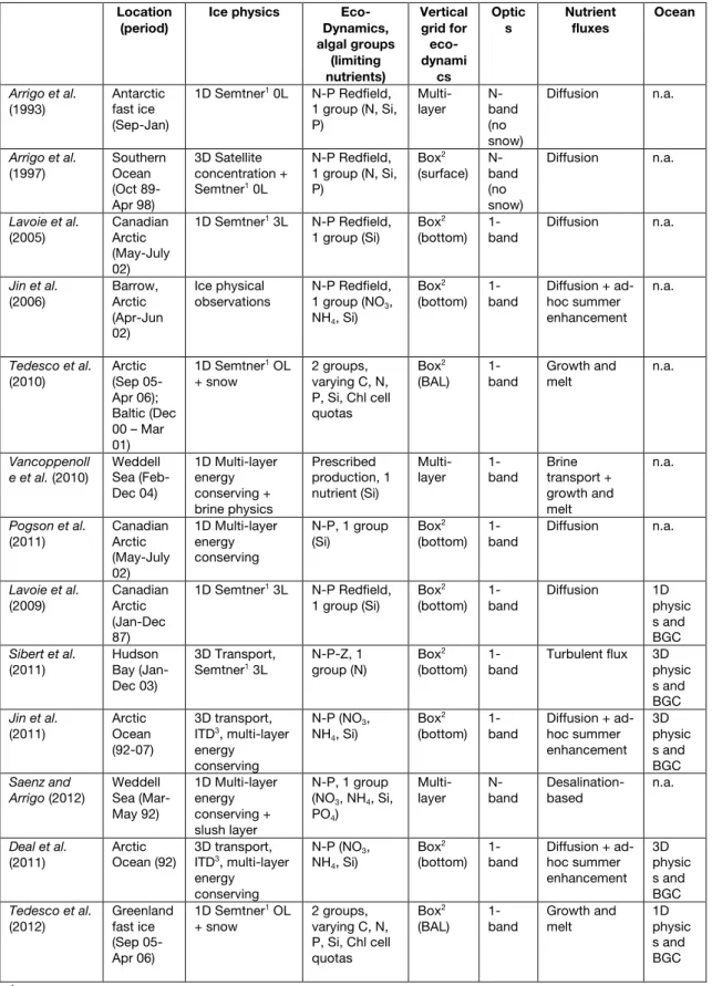
4. Modelling and up-scaling the role of sea ice in the marine biogeochemical cycles 23
5. Discussion and outlook 25
References 26
Abstract
Observations from the last decade suggest an important role of sea ice in the global
biogeochemical cycles, promoted by (i) active biological and chemical processes within the
sea ice; (ii) fluid and gas exchanges at the sea ice interface through an often permeable sea ice
cover; and (iii) tight physical, biological and chemical interactions between the sea ice, the
ocean and the atmosphere. Photosynthetic micro-organisms in sea ice thrive in liquid brine
inclusions encased in a pure ice matrix, where they find suitable light and nutrient levels. They
extend the production season, provide a winter and early spring food source, and contribute to
organic carbon export to depth. Under-ice and ice edge phytoplankton blooms occur when ice
retreats, favoured by increasing light, stratification, and by the release of material into the water
column. In particular, the release of iron – highly concentrated in sea ice – could have large
effects in the iron-limited Southern Ocean. The export of inorganic carbon transport by brine
sinking below the mixed layer, calcium carbonate precipitation in sea ice, as well as active
ice-atmosphere carbon dioxide (CO2) fluxes, could play a central role in the marine carbon cycle.
Sea ice processes could also significantly contribute to the sulphur cycle through the large
production by ice algae of dimethylsulfoniopropionate (DMSP), the precursor of sulfate
aerosols, which as cloud condensation nuclei have a potential cooling effect on the planet.
Finally, the sea ice zone supports significant ocean-atmosphere methane (CH4) fluxes, while
saline ice surfaces activate springtime atmospheric bromine chemistry, setting ground for
tropospheric ozone depletion events observed near both poles. All these mechanisms are
generally known, but neither precisely understood nor quantified at large scales. As polar
regions are rapidly changing, understanding the large-scale polar marine biogeochemical
processes and their future evolution is of high priority. Earth system models should in this
context prove essential, but they currently represent sea ice as biologically and chemically
inert. Paleoclimatic proxies are also relevant, in particular the sea ice proxies, inferring past sea
ice conditions from glacial and marine sediment core records and providing analogs for future
changes. Being highly constrained by marine biogeochemistry, sea ice proxies would not only
contribute to but also benefit from a better understanding of polar marine biogeochemical
cycles.
1. Introduction
Past and on-going climatic changes are amplified in the polar regions [Holland and Bitz, 2003]. Current climate changes, associated with large-scale anthropogenic emissions of greenhouse gases, involve a warming of the ocean, changes in its chemical composition, as well as a dramatic sea ice retreat in the Arctic [Comiso et al., 2010]. Future changes in the polar seas and continued sea ice retreat [Arzel et al., 2006] will affect future marine biogeochemistry, with important feedbacks on climate and consequences for marine ecosystems, some of which have already been observed [e.g., Montes-Hugo et al., 2009;
Wassmann et al., 2011]. Paleo-climate studies
indicate that past climatic and atmospheric composition changes were associated with extensive modifications in the polar oceans, in terms of circulation, sea ice cover and chemical composition [Crosta et al., 1998; Sarnthein et al., 2003; de Vernal et al., 2005; Sigman et al., 2010]. While a seasonal ice cover should subsist in the future [Armour et al., 2011], the future large-scale biogeochemical dynamics of the polar oceans and in particular the contribution of sea ice are difficult to predict.
Ocean biogeochemistry exerts a large control on atmospheric chemistry and climate: by
absorbing about a fourth of anthropogenic carbon dioxide (CO2) emissions [Sabine et al.,
2004], the ocean dampens global warming. The polar and sub-polar oceans are of central importance as they support most of the oceanic CO2 uptake [Takahashi et al., 2009]. Air-sea
carbon exchanges are ultimately driven by two main categories of processes: the solubility and biological pumps. The solubility pump is the ensemble of physical and chemical processes driving CO2 dissolution and outgassing. The
biological pump is driven by (i) the fixation of inorganic carbon into organic matter and its export to depth by sinking plankton material and (ii) the formation of calcium carbonate (CaCO3)
via calcification, releasing CO2 [Sigman et al.,
2010]. While the natural carbon cycle is largely driven by the biological pump [Sarmiento and
Gruber, 2006], the uptake of anthropogenic
carbon can be, so far, almost entirely explained by physical and chemical processes [Prentice et
al., 2001]. The oceanic CO2 absorption capacity
decreases with increasing oceanic CO2 burden,
but may also be reduced because of future anthropogenic climate change (decreasing solubility and increased upper ocean stratification), hence amplifying global warming [Friedlingstein et al., 2006]. The ocean suffers from the increase in its CO2 burden: more
dissolved CO2 acidifies the ocean [Doney et al.,
2009], threatening sensitive and essential marine species, with potential consequences for entire marine food webs. Besides absorbing CO2, the
ocean is also a preferential site for dimethylsulfide (DMS) emissions. In the atmosphere, DMS acts as a precursor of acidic aerosol sulfates which as cloud condensation nuclei have a potential cooling effect on the planet [Charlson et al., 1987; Watson and Liss, 1998].
Sea ice – the ice forming from the freezing of
seawater [WMO, 1970] – is one of the largest known biomes on Earth [Dieckmann and Hellmer, 2010], covering about 7% of the World Ocean, with remarkable seasonal variations seen in both hemispheres [see Comiso, 2010, for a review]. The Arctic sea ice pack has lost about 30% of its summer coverage over the last thirty years [e.g.,
Comiso, 2010] with a spectacular culmination in
2012. This could lead to a summer ice-free Arctic Ocean by the middle of this century [e.g.,
Massonnet et al., 2012]. The Antarctic sea ice
extent has slightly increased over the last thirty years (~1% per decade). However, regional variability is large: increases in the Ross and Weddell Sectors exceed the strong retreat in the Amundsen-Bellingshausen regions [Stammerjohn
et al., 2012]. In addition, the Antarctic sea ice
extent is consistently projected to significantly decrease by the end of this century [Arzel et al., 2006]. The implications of sea ice retreat on the future oceanic capacity to absorb CO2 and emit
DMS, as well as the consequences for climate change, ocean acidification and marine ecosystems, are poorly understood.
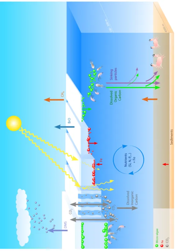
Focussing on sea ice processes relevant to polar marine biogeochemistry (see Figure 1) is first motivated by the potentially significant influence of sea ice on air-sea gas exchanges.
Seen as an impervious cap, sea ice would drastically reduce air-sea CO2 exchange
[Stephens and Keeling, 2000]. However this is hardly the case in practice, because of the
presence of open water within the pack (leads and polynyas), providing pathways for atmosphere-ocean gas exchanges [Morales
Maqueda and Rahmstorf, 2002]. Sea ice itself is
permeable when warm enough [e.g., Golden et
al., 1998], supporting gas exchanges [e.g., Delille et al., 2007; Nomura et al., 2010; Papakyriakou and Miller, 2011] and acts as a source for some
gases, for example DMS [Zemmelink et al., 2008] and potentially Bromine Oxide (BrO) [e.g.,
Simpson et al., 2007]. Until now, the research
community has mainly been interested in the study of biogenic and climatically significant gases (i.e., N2O, O2, CO2, DMS) [e.g., Delille et al.,
2007], although there is growing interest in research on other gases such as Br components, which influence polar atmospheric chemistry [e.g., Simpson et al., 2007] and methane (CH4), a
strong greenhouse gas that is present in gas bubbles released from anoxic sediments to the water column and sea ice [Shakhova et al., 2009]. A second process of interest is the sinking to depth of CO2-rich brine (e.g., richer than
seawater), released into the surface ocean during sea ice formation [Rysgaard et al., 2007].
This process should be among the important mechanisms contributing to the ocean CO2 sink,
not only today [Rysgaard et al., 2011], but also during the last glacial maximum [Bouttes et al., 2010].
In addition, mounting field observations show
dynamic biogeochemical processes in the sea ice zone [Thomas and Dieckmann, 2010], with
potential impacts on open ocean biogeochemistry and atmospheric composition. Sea ice microbial communities are present, and often thrive, in a network of liquid saline brine inclusions distributed within a pure ice matrix (see Figure 2), providing a habitat that is both stable and ventilated by nutrient-rich seawater, depending on the complex brine flow through the ice [e.g., Vancoppenolle et al., 2010]. Organic carbon is produced by ice algae via photosynthesis in specific light, nutrient and temperature conditions, to which the organisms are usually adapted and acclimated. Ice algae can also produce copious amounts of dimethylsulfoniopropionate (DMSP), the precursor of DMS, an osmotic regulator and a cryoprotectant [e.g., Tison et al., 2010]. Finally, iron concentrations in sea ice can be much higher than in the ocean and sea ice can act as a
seasonal reservoir in the Southern Ocean [Lannuzel et al., 2007; 2011]: growing sea ice incorporates large amounts of iron, later released into surface waters when the ice melts. This seasonal process may temporarily relieve iron limitation on phytoplankton growth, notably in the Southern Ocean [Lancelot et al., 2009], a key player in the marine carbon cycle [Sarmiento and
Gruber, 2006; Sigman et al., 2010], but also in the
Bering Sea [Aguilar-Islas et al., 2008]
Sea ice proxies integrate information from
biological, chemical and physical processes occurring in the polar oceans in an attempt to reconstruct past sea ice conditions [see Armand
and Leventer, 2010, for a review]. Many sea ice
proxies rely on assumptions related to the biogeochemical properties of the polar oceans, as recorded in marine sediment or glacial ice cores. For instance, changes in diatoms and dinoflagellates community composition, attributed to the open ocean-sea ice zone transition, are used to reconstruct past sea ice characteristics. Crosta et al. [2008], de Vernal et
al. [2005] and Müller et al [2009], based on
marine sediment core data, use diatom frustules, dynocysts and biomarkers specifically produced by sea ice-associated diatoms and open water phytoplankton, respectively. Curran et al. [2003] and Wolff et al. [2006] use the concentration of methane-sulphonic acid (MSA), an atmospheric by-product of DMS emission in the sea ice zone; and sea salt sodium from glacial ice core data, respectively. However, Hezel et al. [2011] – in an attempt to model the sulphur cycle in the Southern Ocean – find that the presence of sea ice does not exert the dominant control on the interannual variability in DMS emissions. This, combined with the longer simulated lifetime of MSA and DMS in the atmosphere in the high latitudes, raises questions about the applicability of MSA as a proxy for the global Antarctic sea ice extent. Hence, it is apparent that reliable estimates of past sea ice coverage require a proper understanding of present-day large-scale biogeochemical processes occurring in the polar oceans. Conversely, reconstructions of past sea ice extent could enhance our understanding of past polar marine biogeochemistry and reduce uncertainty in future projections of the physical, biological and chemical characteristics of the global ocean.
In this paper, our goal is (i) to review recent advances and caveats in the observation and modelling of the processes driving the dynamics of chemical elements and biological material in the sea ice zone that are relevant to large-scale polar biogeochemical cycles, (ii) to examine the challenges that we face to upscale those processes and understand their role in the global marine biogeochemical cycles, and (iii) to discuss how the growing fields of sea ice biogeochemistry and sea ice paleo-proxy development could synergistically evolve and contribute to each other. We first revisit the physical forcings of relevance to large-scale sea ice biogeochemical processes (Section 2). In Section 3, we summarize recent information on some of the key sea ice biogeochemical properties and processes, with particular focus on their potential large-scale impact and on the associated uncertainties. In Section 4, we review the modelling approaches that have been used to represent polar marine biogeochemical processes. Finally, in Section 5, we give directions for future research with respect to sea ice proxies.
2. Physical controls on sea ice biogeochemistry
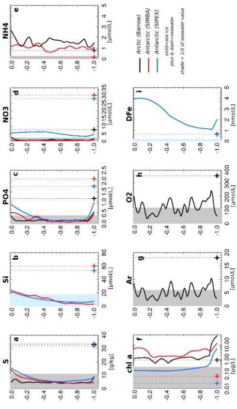
An analysis of sea ice vertical profiles of the most relevant biogeochemical tracers reveals contrasting behaviours (Figure 3). Inorganic macro-nutrients generally conservatively follow salinity, with concentrations much smaller than seawater values in bulk ice. Significant deviations in nutrient concentrations as compared to salinity are associated with biological activity. Gases such as argon (Ar) and oxygen (O2)have relatively
higher and more variable concentrations, compared to ice salinity, because of the formation of gas bubbles. However their concentrations are still below seawater values, except sometimes near the surface. Organic matter and dissolved iron typically show higher concentrations in sea ice than in the underlying ocean. The vertical profiles of biogeochemical sea ice properties reveal the disparity in the physical and biogeochemical processes driving them, which we review hereafter.
Physical processes provide the first set of constraints for biogeochemical developments in sea ice as envisioned by Ackley and Sullivan [1994]. In this section, we cover the aspects of
sea ice physics that we consider relevant for biogeochemistry, in both hemispheres.
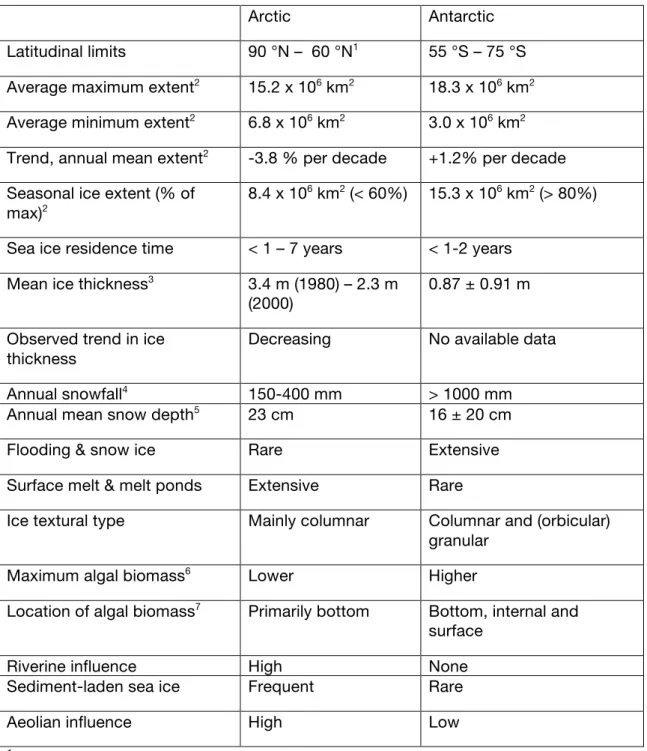
2.1 Large scale sea ice characteristics
Some differences in the characteristics of the polar oceans ice covers (see Table 1 for a summary) are driven by the strong differences in their regional geographic, geo-morphological and geophysical settings [e.g., Eisenman, 2009]. The Arctic Ocean is a high latitude (>65°N) semi-enclosed basin with only limited connection and exchange with the world’s oceans. It is characterized by extensive continental shelves, serving as important areas for sea ice formation and for primary productivity. In contrast, the Southern Ocean is circumpolar, connecting the Atlantic, Indian and Pacific Oceans and showing an ice cover ranging over 55–75°S, i.e., at lower latitudes when compared to the Arctic. The Antarctic continental shelf area is relatively narrow, and extensive areas of sea ice formation are located over deep waters [Dieckmann and
Hellmer, 2010].
Ice extent, monitored from satellites continuously since 1979, varies seasonally more substantially in the Antarctic than in the Arctic. Arctic first-year sea ice cover only makes about half of the total ice extent, while in Antarctica first-year sea ice largely dominates. Over 1979-2009, the annual mean Arctic sea ice extent has been rapidly decreasing by almost 4% per decade, while in the Southern Hemisphere, ice extent has slightly increased by about 1% per decade [Comiso, 2010]. Regional scatter in the trends is significant in both hemispheres. In particular, the Southern Hemisphere increase has to be viewed in regard to strong inter-regional differences: the sharp decrease in the Amundsen/Bellingshausen sector is slightly more than compensated by increases in the Ross, Weddell and Indian sectors [Stammerjohn et al., 2012]. Changes in the timing of sea ice retreat and freeze-up have significant and regionally dependent impacts on primary production [Arrigo et al., 2008b; Montes-Hugo et
al., 2009; Stammerjohn et al. 2008] and
associated marine food webs [Grebmeier et al., 2006; Moreau et al., 2010].
As sea ice is much thinner than it is wide, vertical exchange of biogeochemical material is of primary importance. Ice thickness, however, is more difficult to observe from space than ice extent, and hence global ice thickness data are
relatively scarce. In the Arctic, combined information from upward-looking sonars onboard submarines as well as satellite laser altimeters suggests a decrease in ice thickness from 3.64 m in 1980 to 1.85 m in 2008 in the Arctic Ocean [Kwok and Rothrock, 2009]. In the Southern Hemisphere, the most reliable source of information for ice thickness, the ASPeCt (Antarctic Sea ice Processes and Climate) database, a compilation of ship-based visual observations, suggests a mean ice thickness of 0.87 ± 0.91 m [Worby et al., 2008] over 1981-2005. Because of sampling limitations, temporal changes cannot be derived from the ASPeCt database, but on-going progress in remote sensing techniques is being made towards that goal. A recent model study including satellite ice concentration assimilation suggests an increasing Antarctic sea ice volume by 5.6 ± 5.3 % per decade over 1980-2008 [Massonnet et al., in revision].
During its formation, sea ice incorporates biogeochemical material (e.g., macro-nutrients, iron, organic matter, sediments), which is stored, transformed, and later released in seawater when the ice melts. In addition, organic matter accumulates in the sea ice as a result of auto- and heterotrophic production. Therefore, sea ice drift, induced by winds and ocean currents, horizontally redistributes biogeochemical material. Ice drift is observed using drifting buoys as well as satellites by comparing two subsequent satellite images [Kwok et al., 1990]. Satellite-derived maps of large-scale sea ice drift patterns can be found in Emery et al. [1997]. Ice velocity is on average between 6 and 7 km/day in the Arctic and has been increasing by 17% per decade in winter over 1979-2007 [Rampal et al., 2009]. In the Antarctic, ice velocity typically ranges between 8 and 9 km/day [Heil et al., 2006], while wind patterns over the last two decades have significantly changed [Holland and
Kwok, 2012]. The consequences of ice transport
include the potential initiation of phytoplankton blooms induced by the storage and release of iron in the iron-limited Southern Ocean marginal ice zones [Lancelot et al., 2009; Lannuzel et al, 2010]. Ice transport also involves that the material found in marine sediment cores used in paleoclimate proxies may reflect the conditions a few hundreds to thousands of kilometres away from where the core was extracted.
2.2 Sea ice mass balance
Large-scale variations in sea ice mass are driven by thermodynamic and dynamic processes, which all affect the ice-ocean exchanges of biogeochemical material. Several mechanisms contribute to a net gain of ice mass. (i) Small unconsolidated (frazil) ice crystals forming from super-cooled water either aggregate at the ocean’s surface or adhere onto pre-existing ice [Martin, 1981; Smedsrud, 2002]. (ii) An existing ice cover over quiescent waters grows from the base by congelation if the upward conductive heat flux is higher than the oceanic heat input [Maykut and Untersteiner, 1971]. (iii) Snow ice forms by the refreezing of slush at the snow-ice interface. Slush forms from the infiltration of seawater and brine at the base of the snow pack, when snow is deep enough to depress the ice surface below sea level [e.g., Maksym and
Markus, 2008]. (iv) Superimposed ice forms if
snow melt water, percolating downwards, refreezes deeper in the snow or at the snow-ice interface, where temperature is lower than freezing [e.g., Nicolaus et al., 2009]. The ice formation mechanism can be tracked from specific textural and oxygen isotopes (d18O)
signatures: granular type for frazil, columnar type for congelation, granular with low d18O for
snow-ice formation, and polygonal granular for superimposed ice formation [Weeks and Ackley, 1986; Eicken, 1998; Tison et al., 1998; Haas et al., 2001; Tison et al., 2008]. Depending on the energetic constraints at the interfaces, ice can melt at its surface, at its base, and from the lateral edges of the ice floes.
Changes in the thermodynamic regime of the Arctic sea ice cover have been observed. In the 20th century, the Arctic sea ice mass balance was
driven mostly by basal congelation growth and surface melt [Untersteiner, 1961]. In contrast, over the last two decades, the shares of basal and surface melt have been comparable. Thinner ice fosters the summer reduction in ice concentration, which in turn increases basal melt through to the ice-albedo feedback, as observed [Perovich et al., 2003; Perovich et al., 2007] and simulated [Vancoppenolle et al., 2009b]. Because the long-term ice retreat is more pronounced in summer than in winter [see, e.g., Deser and Teng, 2008], the amplitude of the seasonal cycle of Arctic sea ice extent has been increasing, which means that the total annual sea ice growth and
melt has been increasing and should continue to increase in the future [e.g., Holland et al., 2006]. In the Southern Ocean, observations and models indicate that ice formation mechanisms are more diverse than in the Arctic: congelation, frazil ice and snow-ice formation all contribute significantly [Worby et al., 1996; Jeffries et al., 1997;
Vancoppenolle et al., 2009b]. The direct exposure
of the Southern Ocean sea ice pack to ocean swell results in a higher contribution of frazil ice than in the Arctic, associated with so-called pancake ice formation [Lange et al., 1989]. Because Antarctic air masses are relatively cold and dry [Andreas and Ackley, 1982], and because the ocean heat flux is much larger than in the Arctic [e.g., McPhee, 2008], basal ice melt largely overcomes surface melt in the Southern Ocean [Vancoppenolle et al., 2009b; Maksym et al., 2012]. Lateral melting is confined to the zones where ice floes are sufficiently small [Steele, 1992; Perovich et al., 2003] and has not been clearly evidenced as a significant large-scale mass balance contributor.
Without dynamical deformation processes, the sea ice would be relatively uniform. However, sea ice dynamics introduce small-scale variations in ice thickness through opening (the creation of leads and polynyas), rafting (the overriding of two ice plates on top of each other) and ridging (the piling of broken ice pieces into pressure ridges) [see Tuhkuri and Lensu, 2002]. Ridging and rafting do not induce a net change in sea ice volume, but change the sea ice landscape and the areal distribution of ice thickness. Pressure ridges and the constant formation of new ice in recently opened water due to exposure to cold air induces high variability in ice thickness at subfloe scales [Thorndike et al., 1975]. In the Arctic, models suggest that slightly less than half of the ice volume lies within pressure ridges, while rafted ice contribution is likely very small [Mårtensson et al., 2012]. In the Antarctic, observations suggest a significant influence of deformation processes on the thickness distribution of Antarctic sea ice [Worby et al., 2008], but a proper quantification of the volumetric contribution of deformed ice has still yet to come. As the meridional change in zonal stress associated with the transition from the Antarctic Circumpolar Current to the coastal East Wind Drift induces a generally divergent circulation in the Antarctic sea ice zone, open
water is more prevalent in winter in the Antarctic sea ice pack (>20% of extent) than in the Arctic (~10%) [Gloersen et al., 1993].
Sea ice thermodynamic growth and mechanical redistribution provide important controls on sea ice and upper ocean biogeochemistry. Columnar ice growth at the ice base [Notz and Worster, 2009] and snow ice formation associated with surface flooding trap salt [Maksym and Jeffries, 2000; Vancoppenolle et al., 2010], as well as dissolved and particulate material [Krembs et al., 2001; Giannelli et al., 2001] initially present in seawater, promoting the development of bottom and surface ice algal communities. Rising frazil ice crystals are known to harvest some of the available particulate material suspended in the water column and to incorporate it in the ice [Martin, 1981; Garrison et al., 1983; Ackley and
Sullivan, 1994]. Due to brine drainage, a large
part of dissolved material is quickly released to the ocean (see Section 2.3). Melting sea ice releases material in seawater [Riebesell et al., 1991; Michel et al., 1996], which affects both planktonic and benthic communities.
Ridging and rafting must affect ice algal communities significantly, but to what extent is not well understood. The analysis of a circumpolar Southern Ocean sea ice chlorophyll database suggests that at least a third of the biomass in the Southern Ocean pack ice is associated with internal communities living in deformed ice [Meiners et al., 2012]. Ice deformation by ridging and rafting vertically redistributes biogeochemical material [Horner et
al, 1992]. Rafting brings algal communities that
were previously near the ice base to the ice interior, while ridging randomly redistributes material within the pressure ridges. Ridges are initially highly porous: about 30% of ridged ice volume is trapped seawater, which should expose the newly dispersed communities to large amounts of macro-nutrients and therefore make this habitat very productive, but this is still a speculation at this stage. In the Arctic, this would also largely depend on the amount of nutrients initially present in seawater, which is controlled by vertical mixing and upwelling in the underlying ocean.
2.3 Factors influencing light availability in sea ice
The strong seasonality in light conditions in polar regions, from complete winter darkness to 24-h daylight near the poles, sets constraints on quantum irradiance available to primary producers, or Photosynthetically Active Radiation (PAR). The factors influencing radiation transfer through sea ice are mainly the snow cover, melt ponds, as well as the presence of sediments, pollutants and biological material in the ice. The snow cover above sea ice can be very reflective (hence opaque) and is therefore of primary importance in spring. The evolution of snow depth is governed by snowfall, sublimation, melt and metamorphism. In addition, wind redistributes snow from undeformed ice towards the vicinity of rough topographic features such as pressure ridges, while some blowing snow can be lost on its way to open water [Massom et al., 2001; Sturm and Massom, 2010; Leonard and
Maksym, 2011]. The irregularities of the sea ice
surface, combined with the spatially dependent snowfall rate, snow thermodynamics and wind redistribution induce large variations in snow depth even at sub-meter scales [see, e.g., Mundy
et al., 2005; Lewis et al., 2011]. This has
important consequences for light-dependent biological process in and under ice, as snow attenuates light very efficiently.
Measurements of radiation extinction coefficients in the visible waveband fall within 6-80 m-1 for all
types of snow [Hamre et al, 2004; Järvinen and
Lepparanta, 2010], within 0.8-1.5 m-1 for natural
sea ice [e.g. Light et al., 2008; Nicolaus et al., 2010], and within 0.02-0.49 m-1 for seawater [e.g., DeGrandpre et al., 1996]. Hence a few
centimetres of snow can attenuate as much shortwave radiation as a meter of sea ice. Field studies suggest that, within a floe, ice algae are found where light intensity is the strongest [Rysgaard et al., 2001], with the thickness of the combined snow-ice system being the most important factor controlling the algal biomass patch sizes at subfloe scales (~10 m) in the absence of nutrient limitation [Gosselin et al., 1986; Rysgaard et al., 2001]. Historical data of Southern Ocean sea ice chlorophyll [Meiners et
al., 2012] indicate that low ice algal biomasses (<
1mg chla/m2) constitute ~30% of observations,
even when sea ice is overall biologically productive, which is in part due to light
attenuation by snow. Besides its effect on light attenuation, snow depth also controls the thermal field and hence the intensity and depth of brine convection rates [Notz and Worster, 2008]. Snow depth also determines the formation of snow ice and the flooding of the snow base by seawater, which can bring nutrients near the ice surface and promote the development of surface layer communities [Fritsen et al., 1994].
The Antarctic sea ice pack experiences some of the largest snowfall rates on Earth, hence high snow-loading results in frequent flooding of Antarctic sea ice, fostering snow ice formation [Maksym and Markus, 2008]. In contrast, snowfall on Arctic sea ice is generally lower than in the Antarctic, whereas sea ice is generally thicker, and therefore requires a heavier snow cover to flood. Therefore, surface flooding is rather rare in the Arctic. In the Northern Hemisphere, due to the proximity of pollutant sources, snow falling onto sea ice can result in deposition and accumulation of NO3, NH4 and soot [Ehn et al.,
2004; Nomura et al., 2011].
The incorporation of sediments, rare in Antarctic sea ice but frequently observed in Arctic sea ice especially near the coasts, strongly affects light availability for ice algae and transmittance of light to the under ice pelagic environment [Light et al., 1998; Gradinger et al., 2009]. Sediment-laden ice has been shown to impact on the spectral light composition and can also delay and inhibit the ice algal spring bloom development [Gradinger et
al., 2009].
Another property of importance for light availability under sea ice is the presence of melt ponds. These are pools resulting from the accumulation of melt water over impermeable sea ice, forming shortly after melt onset [Perovich
et al., 2002b; Polashenski et al., 2012], and
characterized by much lower albedo than bare ice [Perovich and Polashenski, 2012]. Widespread in the Arctic, where they cover about 1.5 million km2 at their summer maximum [Rösel and Kaleschke, 2012], melt ponds are rarely reported
on Antarctic sea ice, because of drier and colder air than in the Arctic [Andreas and Ackley, 1982], favouring evaporation rather than melt water accumulation at the surface [Nicolaus et al., 2009]. Melt ponds efficiently transmit light to the underlying ocean, with transmission values typically an order of magnitude higher than bare
ice [Frey et al., 2011]. Therefore, substantial melt pond coverage changes the ocean’s surface energy budget [Nicolaus et al., 2012] and stimulates under-ice primary productivity [e.g.,
Arrigo et al., 2012]. Melt ponds also host their
own planktonic communities [Horner et al, 1985], but their contribution in the large-scale carbon cycle is likely limited [Lee et al., 2012].
2.4 Controls of fluid transport on biogeochemical tracers
One of the key characteristics of sea ice making it suitable as a microbial habitat is the presence of liquid inclusions of saline brine, which are at
least near the ice base connected with the underlying ocean, providing pathways for nutrient supply [Reeburgh, 1984, Petrich and Eicken, 2010] and gas exchange [Delille et al., 2007;
Tison et al., 2010; Loose et al., 2011]. The salt
trapped within sea ice during formation is hardly incorporated into the ice crystalline lattice [Weeks
and Ackley, 1986] and rather remains dissolved in
brine [see Hunke et al., 2011, for a review]. The bulk salinity of sea ice (i.e., for the combined ice and brine pockets) is usually much less than seawater, although brine salinity can be much higher. Brine salinity strongly increases with decreasing temperatures to maintain phase equilibrium within sea ice, while the brine volume fraction increases with temperature and ice bulk salinity [Assur, 1958; Cox and Weeks, 1983;
Hunke et al., 2011]. As sea ice ages, much of the
brine is lost from the ice, decreasing bulk salinity and brine volume.
Above a ~5% threshold in brine volume, the brine network connects and fluid permeability of sea ice drastically increases [Golden et al., 1998], enabling fluid transport through sea ice. In practice, the vertical structure of fluid permeability in sea ice is seasonally dependent, following temperature changes modulating the vertical position of the 5% brine volume contour. Near the ice base, where the ice is warm and saline, the brine network is virtually always in connection with the underlying ocean. In winter, the 5% brine volume contour is at about one third of the ice thickness from the ice-ocean interface, hence only the lowermost part of the ice is permeable [Vancoppenolle et al., 2007;
Notz et al., 2009]. In summer the 5% brine
volume contour moves upwards in the ice due to warming. Full-depth connectivity happens in
spring once the ice is warm enough [Jardon et
al., 2013]. In summer, in particular in the Arctic,
strong desalination of sea ice due to flushing can reduce the brine volume below 5% over most of the sea ice depth [Vancoppenolle et al., 2007]. Recent results suggest life in sea ice also exerts some control on brine inclusions. Exopolymeric polysaccharides (EPS) released by ice algae and bacteria [Krembs et al., 2002a] change the size and shape of brine inclusions, reduce fluid permeability and increase salt retention in sea ice [Krembs et al., 2011]. To which extent ice algae affect fluid transport through sea ice in natural conditions is not clear yet and not represented in current thermodynamical theories of the sea ice microstructure.
The markers of biochemical activity – nutrients, gases, micro-organisms – are all influenced by the sea ice microstructure. In practice, they are considered as passive tracers, i.e., influenced
by their physical environment but not affecting the sea ice thermodynamic state. Their abundance in the ice can be characterized using
bulk molar volumetric concentration C(z,t), i.e.,
the number of moles of tracer per unit volume of sea ice. This volume has to be small enough so that a single brine volume fraction is representative of the volume, but large enough so that individual brine inclusions are averaged [Jeffery et al., 2011]. Changes in C are driven by physical transport (Sφ) and by biological and
chemical source and sinks (Sβχ):
, (1)
Physical transport depends on the tracer of interest, which can be of three different kinds:
dissolved, gas, or particulate.
Dissolved tracers.
Dissolved tracers (as dissolved macro-nutrients and inorganic carbon) behave like salt, i.e., their concentration in pure ice is nil and they are transported vertically with brine motion. For these tracers, the brine concentration Cbr, or the
number of moles of tracer per unit volume of liquid brine, is introduced as:
where e is brine volume fraction. In the sense that sea ice is a two-phase, reactive porous medium, it constitutes a mushy-layer [Notz and Worster, 2009]. Mushy-layer theory provides a theoretical framework to express changes in C due to brine transport (see below), which are currently formulated as functions of e and Cbr [see, e.g., Vancoppenolle et al., 2010; Jeffery et al., 2011].
Brine transport. Fluid transport in brine
inclusions drives a net loss of salt from the sea ice to the ocean. Fluid transport through the ice is controlled by the vertical thermo-haline structure of sea ice, which determines both the vertical stability of the brine network and its connectivity. Only gravity drainage and flushing are believed to contribute to any measurable net loss of salt [Untersteiner, 1968; Notz and Worster, 2009]. Gravity drainage refers to the natural
convection of salty, heavy brine and its replacement with less dense underlying seawater, which is limited to where the ice is permeable and when the brine salinity decreases from the top of the ice downward (when air temperature is below seawater freezing point). This salinity gradient leads to an unstable density gradient of the interstitial brine, prone to convection, primarily through vertical brine channels – liquid conduits extending through the ice which naturally form during sea ice formation [Niedrauer and Martin, 1979; Wells et al., 2011]. Gravity drainage results in an important net rejection of salt from the sea ice into the ocean.
Flushing is the dominant desalination process
during the Arctic summer. This process refers to the “washing out” of salty brine by relatively fresh surface melt water that percolates into the pore space during summer [Untersteiner, 1968]. Because surface melting is not frequent in the Antarctic, flushing is rarely observed there [see
Vancoppenolle et al., 2009a and references
therein]. Flushing also expels dissolved material from the ice during the melt period, which typically ends the ice algal season in the Arctic [e.g., Riedel et al., 2008].
A last brine motion mechanism that potentially can play a role is forced convection. Forced
convection in the lowermost parts of the brine network is driven by the pressure difference induced by the shear of ocean current under sea ice, as suggested by theoretical and experimental
studies [Neufeld, 2008]. Forced convection may bring in and redistribute salt and nutrients in sea ice, but when, how and how much have not yet been evaluated. Forced convection could occur for instance due to strong tidal currents and play an important role when the brine network is stable in summer. This is corroborated by the hypothesized control of tidal forcing on nutrient supply to the sea ice, required to explain the high ice algal biomass accumulation observed in the bottom layers of fast ice in Resolute Bay, in the Canadian Arctic Archipelago [Cota et al., 1987;
Cota and Horne, 1989]. Significant progress on
the fundamental understanding of brine transport mechanisms is still required [see, Hunke et al., 2011].
Brine transport and nutrients. Most
macro-nutrients are, like salt, dissolved in brine. Hence, fluid transport removes nutrients from (or supplies them to) the ice interior [Reeburgh, 1984; Vancoppenolle et al., 2010]. Salt is trapped within sea ice during basal accretion and surface flooding. During basal ice growth, the salinity field is continuous across the ice-ocean interface, hence there is no immediate segregation of salt from the ice to the ocean [Weeks and Ackley, 1986] at the advancing front [Notz and Worster, 2009]. All nutrients included in the freezing seawater should conservatively follow salt and be incorporated into forming ice. Flooding of the base of the snow layer under negative freeboard conditions occurs either (i) laterally via the infiltration of seawater through fractures associated with open water, deformed ice and thermal cracks, or (ii) vertically via the percolation of brine through brine channels [Maksym and
Jeffries, 2000]. Flooding is a source of salt to the
ice surface [Eicken et al, 1992] and should bring and redistribute nutrients near the ice surface.
Interactions between transport and biochemical sources and sinks. Nutrient
concentrations in sea ice are in part controlled by brine dynamics but also depend on ice algal uptake and remineralization processes due to heterotrophic activity. Because nutrients are non-conservative elements, affected by biological processes acting as nutrient sources or sinks, the effect of gravity drainage on nutrients can deviate from its effect on salt. Depending on whether the concentration of nutrients in brines is higher or lower than in seawater below, gravity drainage
rejects or supplies nutrients to the sea ice [Vancoppenolle et al., 2010]. In theory, as long as the air temperature is below the seawater freezing point, which implies an unstable brine salinity profile (i.e., brine salinity increases upwards), gravity drainage can supply nutrients – if depleted – to the permeable sections of the ice, which are in most cases restricted to the lowermost 10 cm of the ice, but can extend further up within the ice in late spring [see, e.g.,
Zhou et al., in revision].
Gas tracers
Like salt and nutrients, dissolved gases are incorporated in sea ice and concentrated into brine inclusions during ice formation (basal congelation, snow-ice, frazil) [Matsuo and Miyake, 1966; Glud et al., 2002; Tison et al., 2002], while gas bubbles coming from the ocean below penetrate the ice via the open brine network [Tsurikov, 1979]. Most of the gases are then quickly released into the underlying ocean through convective brine release, where they partly sink, following dense waters convection [Killawee et al., 1998; Rysgaard et al., 2007; Sejr
et al., 2011] or escape upwards through the open
water-atmosphere interface [Nomura et al., 2006;
Loose et al., 2011].
Gas tracers easily form bubbles within growing sea ice, because of two synergetic effects of decreasing ice temperature: (i) brine volume decreases, which increases dissolved gas concentration in brine possibly above gas solubility [Zhou et al., in revision]; and (ii) gas solubility decreases. The latter effect is because brine salinity and temperature are coupled: the increase in solubility due to cooling is over-compensated by the decrease due to increasing brine salinity [Thomas et al., 2010]. Above saturation, if the sum of all dissolved gases partial pressures is higher than the local hydrostatic pressure, bubbles can nucleate and accumulate in the direct vicinity of sea ice inclusions [Tison et al., 2002; Light et al., 2003]. Internal melting also promotes gas bubble formation: melting involves a ~10% volume reduction, leaving a void where gas will flow from nearby brine until equilibrium [Perovich and Gow, 1996]. When brine inclusions enlarge in spring and summer, the brine concentration of gases decreases, possibly reaching under-saturation.
This under-saturation can be relieved by inputs from dissolving gas bubbles, as well as from atmospheric and oceanic inputs [Tison et al., 2010; Zhou et al., in revision]. If the ice is permeable, gas bubbles can directly escape to the atmosphere. During the melt season, flushing transports dissolved gases towards the ocean.
Gas tracers (O2, Ar, CO2) are distributed in both
the liquid and gas phases, and their bulk concentration is given by:
, (3)
where Cbub is the contribution of gas bubbles to
bulk ice concentration. The physical transport term (Sφ) in equation (1) includes not only brine
transport (affecting Cbr), but also gas bubble
transport (affecting Cbub).
While the transport of dissolved gas should be similar to that of salt, the transport of gas bubbles, little studied, is likely driven by different
processes, including the buoyant rise of gas bubbles, and their entrapment in the sea ice microstructure [Zhou et al., in revision]. A scaling analysis suggests that gas bubbles should quickly escape out of the ice due to their buoyancy once the brine network opens in spring [Moreau et al., in revision]. Recent observations [Zhou et al., in revision] indicate that the permeability transition for gas bubble transport could occur at a higher brine volume permeability threshold than the commonly accepted threshold of 5% for fluid transport [Golden et al., 1998]. In contrast to the general behaviour of dissolved salt and nutrients, dissolved gases and gas bubbles can cross the ice-atmosphere interface.
Ice-atmosphere gas exchange depends on the
differential partial pressure of gases between brine and the atmosphere, wind speed, ice microstructure and snow properties [Delille, 2006;
Heinesch et al., 2009; Papakyriakou and Miller,
2011; Bowling and Massman, 2011]. When present, snow can act as an intermediate reservoir for gas until wind speed exceeds a given threshold [Bowling and Massman, 2011;
Papakyriakou and Miller, 2011] while, when
absent, brine-atmosphere or melt pond-atmosphere gas exchanges may occur [Semiletov et al., 2004]. The formation of superimposed ice impedes sea ice-atmosphere
gas exchanges [Nomura et al., 2010]. The central question of the partitioning of gas exchange between open water and sea ice has not been resolved yet [see, e.g., Loose et al., 2011; and references therein].
Gas dynamics in sea ice are complicated by biogeochemical processes. These include the metabolic activities (i.e., primary production and respiration) [e.g., Arrigo et al., 2010; Deming, 2010], which produce and absorb biogenic gases such as O2, CO2 and DMS [Gleitz et al., 1995; Glud et al., 2002; Delille et al., 2007; Tison et al.,
2010]. They also include carbonate chemistry, which plays an important role in the dynamics of dissolved inorganic carbon (DIC) in sea ice [Delille, 2006; Rysgaard et al., 2007; Miller et al., 2011a; Geilfus et al., 2012], and the precipitation of calcium carbonate (CaCO3) in the form of ikaite
crystals as recently observed in Arctic and Antarctic sea ice [Dieckmann et al., 2008; 2010].
Particulate tracers
Particulate tracers cannot dissolve in brine.
Their incorporation in the sea ice matrix and actual transport behaviour depends on several characteristics which are not currently well constrained: (i) whether the particles move actively (e.g., flagellates), (ii) whether the particles are transported passively (by moving brine), (iii) whether and how quickly they stick on the walls of brine inclusions or on other impurities, (iv) whether they can get sealed into the sea ice microstructure. For instance, ice micro-organisms combine mobility and attachment onto ice surfaces via the release of EPS and ice-binding proteins [Krembs et al., 2000; Becquevort
et al., 2009; Juhl et al., 2011; Raymond and Kim,
2012].
3. Biogeochemical processes
Active biogeochemical processes in sea ice involve macro-nutrients, trace elements, organic carbon, inorganic carbon, other climatically-significant gases (DMS, methane, nitrous oxide), and atmospheric halogen chemistry, in strong interaction with oceanic and atmospheric processes.
3.1 Organic carbon processes in sea ice
Biodiversity. Sea ice provides a vast habitat for
productive microbial communities consisting of algae, bacteria, archea, heterotrophic protists,
funghi as well as viruses [Horner et al. 1992;
Deming et al., 2010; Thomas and Dieckmann,
2010; Poulin et al., 2011]. Distinct communities are found at the base, in the interior and at the surface of ice floes [see, Horner, 1985; Arrigo et al., 2010]. In terms of biomass, these communities are generally dominated by algae, particularly diatoms during the bloom period. However, heterotrophs can dominate prior to the bloom period, as well as during the winter [Riedel
et al. 2008, Niemi et al., 2011; Paterson and Laybourn-Parry, 2012]. There are over one
thousand protist species known to live in Arctic sea ice, including diatoms, dinoflagellates, chrysophytes, prasinophytes, silicoflagellates, primnesiophytes and chlorophytes amongst others [Poulin et al., 2011]. Pennate diatoms, with morphotypes resembling surface-associated and benthic life-styles, are the dominant sea ice algal group. The arborescent colonial diatom Nitzschia
frigida is the most abundant and the most widely
distributed ice algal species in Arctic first-year ice and therefore is a key sea ice species in the circumpolar Arctic [Różańska et al., 2009]. Other diatom species such as Melosira arctica, which can form meter-long strands attached to the sea ice, can also be overwhelmingly dominant in Arctic sea ice. An important Antarctic sea ice pennate diatom genus is Fragilariopsis, which is commonly found in pack ice habitats and has been widely used as a sea ice proxy [see Armand
and Leventer, 2010; and references therein]. Ice
algae in general extend the duration of the productive season in high latitude ecosystems. This is mostly because ice algae are attached to the ice and therefore not subject to vertical motion in the water column affecting average light exposure of phytoplankton in a mixed layer. Ice algae also provide a critical early season and high-quality food source for the growth and reproduction of pelagic herbivores [Søreide et al., 2010; Flores et al., 2012].
Variability. There is a high spatial and temporal
variability in ice algal biomass and production. The seasonal development of ice algal communities is driven by the strong seasonal physical forcing regime of polar marine environments. During the dark winter at high latitudes, protist abundance is relatively low in sea ice [Günther and Dieckmann, 1999; Niemi et
al., 2011]; however Arctic winter sea ice
assemblages [Niemi et al., 2011]. Ice algae are typically shade adapted and can thrive at very low irradiances. Increasing light levels in late winter trigger the onset of ice-algal blooms [Lavoie et al., 2005; Meiners et al., 2012]. The decline of Arctic ice algal blooms depends on a variety of factors including nutrient limitation by nitrogen [Różańska et al., 2009] and silicic acid [Lavoie et al., 2005], self-shading [Smith et al., 1988], as well as temperature and brine salinity stress [Arrigo and Sullivan, 1992]. Nutrient limitation occurs when supplies are limited, which is promoted by brine stratification at near-freezing temperatures. Decreasing light levels, low temperatures and high brine salinities limit ice algal growth during late autumn and winter. For some high-biomass Antarctic sea ice microhabitats, potential algal growth limitation by depleted CO2, elevated brine pH, and oxygen
supersaturation has been reported [Gleitz et al., 1995; Thomas et al., 2010]. In contrast, heterotrophic processes, e.g., bacterial activity, heterotrophic grazing and excretion, as well as viral lysis of host cells, can result in nutrient remineralization within the sea ice [Gleitz et al., 1995; Papadimitriou et al., 2007; Riedel et al., 2008; Thomas et al., 2010]. Large spatial variability in ice algal activity is found from sub-meter to large scales [Rysgaard et al., 2001; Deal
et al., 2011], due to processes that operate at
micro- (individual pores), meso- (snow distribution) and macro- (nutrient input) scales.
Characterization of biomass and organic carbon. There are several quantities that are
used to characterize the organic matter content in sea ice. Chlorophyll a (chl a), the dominant photosynthetic pigment in marine microalgae, is easily measured fluorometrically, and is the most frequently used indicator of autotrophic biomass. Vertically-integrated concentration of chl a (Ichla),
or areal chlorophyll content, is an indicator of the total biomass per unit area of sea ice [Gradinger, 2009; Meiners et al., 2012]. Ichla is generally
highest in landfast ice, i.e., sea ice that is “fastened” by attachment to the coast, ice shelves, glacier-tongues or locked-in by grounded icebergs. Landfast ice is more productive due to coastal processes that influence nutrient supply, i.e., riverine influence (in the Arctic) and tidal currents, which promote vertical mixing and forced convection in sea ice. Values of Ichla for a given ice core (or a part of it,
depending on authors) range between 1 and 340 mg m-2 in the Arctic and between <1 and 1090
mg m-2 in the Antarctic, which includes both pack
and fast ice [see Arrigo et al. 2010; and references therein]. The highest values probably do not reflect a large-scale measure but rather local maxima. As Ichla estimates presented in the
literature often include only a fraction of the ice thickness, they have to be interpreted carefully. The sea ice particulate organic matter (POM) pool, operationally defined as material retained on glass-fibre filters with a nominal pore size of 0.7 micron, provides a more general measure of organic matter in sea ice, comprised of different fractions including ice algae, some exopolymers, attached bacteria, heterotrophic protists, and detritus. POM is mostly measured as particulate organic carbon (POC) but particulate organic nitrogen (PON) is also used in nitrogen-based budgets and models.
POC and Chl a in sea ice can show strong vertical gradients and can vary spatially and seasonally over 3 orders of magnitude [e.g.,
Kennedy et al., 2002]. POC and Chl a also vary as
a function of the age of sea ice. The distribution of POC in sea ice is usually correlated with that of Chl a, implying that ice algae represent a large part of, and partly produce the POC. However, during fall and winter, sea ice POC and Chl a are decoupled, indicating a significant contribution of non-pigmented biomass (heterotrophs and detritus) [e.g., Meiners et al., 2004; Niemi et al., 2011]. In addition, allochtonous riverine and terrestrial material input in sea ice can be high on Arctic shelves, which influences the POM sea ice signature in Arctic sea ice.
While Chl a is a widely used proxy for ice algal (and phytoplankton) biomass in ecological studies, other cell constituents, such a biogenic silica, a structuring element of diatom frustules, can also be used. Each indicator has advantages and shortcomings. Therefore, a combination of indicators offers the best description of the biomass and physiological state of ice community assemblages. POC indiscriminately measures all of the organic carbon regardless of its physiological (e.g., healthy cells or detritus) or functional (autotrophic or heterotrophic) roles. Chl a specifically targets phototrophic biomass (excluding cyanobacteria), whereas biogenic silica targets diatoms. Overall, since these
indicators change with the composition and physiological status of ice communities, they may not accurately reflect ice algal biomass across different seasons, regions and sea ice habitats.
DOM. Dissolved organic matter (DOM) is a
diverse pool of molecules including carbohydrates, proteins, amino acids as well as more complex substances such as humic substances. DOM is defined as organic matter smaller than 0.2 µm. However, operationally, DOM is often measured as the material that passes through glass-fibre filters with a nominal pore size of 0.7 µm. DOM can be derived from various sources such as viral lysis of cells, inefficient and destructive sloppy-feeding by grazers, with the most important sea ice source being exudation by microalgae. Allochtonous DOM input into marine systems also occurs via rivers transporting complex humic substances into the marine realm. DOM can range in size from monomers to large polymers and can be divided in a biological labile and a relatively stable (refractory) pool. Labile DOM provides an important food source for bacteria channelling energy through sea ice microbial food webs. DOM includes chelating agents that are considered to influence the bio-availability of nutrients, such as iron [Hassler and Schoemann, 2009]. DOC (Dissolved Organic Carbon, measured via catalytic combustion) in the sea ice is often correlated with ice algal biomass and can reach very high concentrations when compared to the pelagic realm. DOC concentrations of up to > 2.5 x 10³ µM have been reported for Arctic
sea ice [Riedel et al., 2008]. DOC concentrations in Antarctic sea ice vary widely with values of up to >1.8 x 10³ µM in melted ice cores [e.g., Thomas et al., 2001; Herborg et al., 2001; Thomas et al., 2010]. As DOC is further
concentrated within sea ice brines, organisms living in brine are exposed to DOC concentrations that are up to 3 orders of magnitude higher than in seawater. Coloured Dissolved Organic Matter (CDOM) constitutes a significant fraction of the sea ice DOM pool and can significantly contribute to the attenuation of sunlight (particularly in the UV wavelength ranges) and serve as substrate for photochemical reactions that can remineralize the CDOM breaking it down into more labile compunds [Belzile et al. 2000; Norman et al., 2011].
EPS. Over the last decade or so, various studies
have shown that part of the organic matter is constituted of gel-like organic substances, often referred to as extracellular polymeric substances (EPS), which can represent up to 70 % of the sea ice POC pool [Krembs et al., 2002a; Meiners et
al., 2003; 2004]. EPS are thought to serve in cell
attachment and motility, act as a buffer against pH/chemical variations, provide protection from grazers and improve sea ice habitability [e.g.,
Krembs et al., 2002a; Meiners et al., 2003; Riedel et al., 2006; Underwood et al., 2010; Krembs et
al. 2011]. Importantly, recent studies on Arctic fast ice have shown that EPS can be retained in sea ice during ice melt in spring when particulate organic carbon is lost from the ice into the underlying water [Riedel et al., 2006; Juhl et al., 2011]. This discontinuous export of organic matter from seasonal sea ice suggests that the released material changes in quality and quantity with the progression of the melt season, which in turn affects its biogeochemical cycling.
3.2 Macro-nutrients in sea ice and in the water column
All macro-nutrients, namely nitrate (NO3-), nitrite
(NO2-), phosphate (PO43-) and silicic acid (Si(0H)4),
are dissolved in brine inclusions, with the notable exception of ammonium (NH4+). Therefore,
nutrient concentrations in bulk ice (C) follow equation (2). For, NH4+, one of the rare ions that
can be trapped within ice crystals during freezing [Weeks, 2010], equation (1) does not apply and its dynamics are different from other nutrients. There are numerous examples of vertical nutrient profiles in sea ice in the literature [see Thomas et
al., 2010, and references therein; and Figure 3,
for indicative profiles]. They indicate that macro-nutrient concentrations in bulk ice are relatively low compared to seawater values. During the ice algal production period, from spring to fall, C usually lies on or below the dilution line [e.g.,
Tison et al., 2008; Zhou et al., in revision], e.g., C/S ≤ Cw/Sw (no superscript refers to sea ice,
superscript w refers to seawater, S is salinity), which indicates a net consumption by photosynthetic organisms, superimposed on the brine dynamics-driven signal. On some occasions, essentially in winter [e.g., Dieckmann
et al., 1991; Zhou et al., in revision], C is above
the dilution line, which suggests significant remineralization. Ammonium concentrations are typically on or above the dilution line, which is