180 DEGREE DOMAIN WALLS AS
A SOURCE OF MAGNETOACOUSTIC EMISSION by
THOMAS WILLIAM ALTSHULER B.S. Rensselaer Polytechnic Institute
(1983)
S.M. Massachusetts Institute of Technology (1988)
Submitted to the Physics Department in Partial Fulfillment of
the Requirements for the Degree of
DOCTOR OF PHILOSOPHY at the
Massachusetts Institute of Technology August 1993
© Massachusetts Institute of Technology 1993 All rights reserved
Signature of Author
Physics Department August 1993
Certified by
Department of
Professor Robert M. Rose Material Science and Engineering Thesis Supervisor
Accepted by
Professor George Koster Chairman Graduate Comittee
MASSACHUSETTS INSTITUTE OF TECHNOLOGY
NOV 02 1993
LIBRARIES
2 180 DEGREE DOMAIN WALLS AS
A SOURCE OF MAGNETOACOUSTIC EMISSION by
THOMAS WILLIAM ALTSHULER Submitted to the Physics Department
on August 30, 1993 in partial fulfillment of the requirements of the degree of Doctor of Philosophy in
Physics ABSTRACT
Magnetoacoustic emission from 180 degree domain walls in magnetic materials is investigated. The result is a theoretical model which predicts that the 180 degree domain wall is a source of elastic radiation. This is contrary to accepted theory. The emission from a planar moving 180 degree domain wall is modeled using a micromagnetic
approach to determine the spin distribution within the domain wall. The continuum spin distribution within the wall has a small component in the direction of motion of the domain wall. The component in the direction of motion is directly proportional to the velocity of the domain wall for velocities small compared to the Walker limiting velocity. Using the spin distribution, a continuum elastic model is developed where the motion of domain walls couples into the crystal lattice via magnetostriction. It is shown that the 180 degree domain wall emits elastic radiation upon acceleration. This is the necessary condition for elastic radiation, i.e., the convective derivative of the non-elastic strain is non-zero.
A transducer is developed to measure the elastic radiation from the accelerating 180 degree domain wall. The transducer is based on a Scanning Tunneling Microscope modified to have sensitivity to surface motion on the order of 10-12 meter with a 5 MHz bandwidth. The tunneling transducer is used to attempt to measure small shear elastic emission from domain walls in a SiFe picture frame single crystal. The magnitude of the emission based on the theoretical model developed in the thesis is approximately the same as the noise limit of the tunneling transducer. Thus no magnetoacoustic emission is measured. Experimental modifications are discussed to enhance the ability to isolate elastic radiation from a moving 180 degree domain wall.
Thesis Supervisor: Professor Robert M. Rose
3 Table of Contents Abstract 2 Table of Contents 3 List of Figures 7 List of Tables 10 Acknowledgement 11 Chapter I: Introduction 12 1.1 Background 12
1.2 Magnetoacoustic Emission: Background 12
1.3 Magnetoacoustic Emission: Models for Emission 13
I.3a Magnetoacoustic Emission: Magnetoelastic Energy Model 13 I.3b Magnetoacoustic Emission: Effects of Applied Stress and
Internal Strain 15
I.3c Magnetoacoustic Emission: Dynamic Inelastic Strain Model 17 I.3d Magnetoacoustic Emission: Creation/Annihilation Model 18 I.3e Magnetoacoustic Emission: 180* Domain Wall Model 19
1.4 Scope of Thesis 20
Chapter II: Magnetic Domain Wall 24
11.1 Introduction 24
11.2 Overview 25
11.3 The Static Domain Wall Equilibrium Equation 27
11.4 The Static Domain Wall 28
II.4a The Static Domain Wall: Magnetic Field Terms 30 II.4b The Static Domain Wall: Closure Domains and the Infinite Crystal 33
II.4c The Static Domain Wall: Uniaxial Material 36
11.5 Effects of the Magnetoelastic Field on a Domain Wall
in a Cubic Material 39
II.5a Magnetostrictive Coalescence of the 180" Domain Wall 41 11.6 Effects of Magnetostatic Energy on the Domain Wall
in a Cubic Material 48
11.7 The Static Domain Wall: Cubic Material with Magnetostatic
Self Energy 51
Chapter III: Elastic Radiation during Magnetization: A Review 55
111.1 Introduction 55
111.2 Previous Emission Models 57
III.2a Previous Emission Models: Magnetoelastic Energy Model 57 III.2b Previous Emission Models: Dynamic Inelastic Strain Model 63 III.2c Previous Emission Models: Creation/Annihilation Models 65 III.2d Previous Emission Models: 1800 Domain Wall Model 67 Chapter IV: Elastic Radiation Emitted by a Moving 180 Domain Wall 71
IV. 1 Introduction 71
IV.2 Dynamic Emission Source 72
IV.3 The Static 1800 Domain Wall 74
IV.4 Magnetization Distribution for the Moving 180 Domain Wall 76
IV.4a The 1800 Domain Wall with Constant Velocity 78
IV.4b The Accelerating 1800 Domain Wall 84
IV.5 Magnetoacoustic Emission from the Moving 1800 Domain Wall 86 IV.5a Green's Function Solution to the Inhomogeneous Wave Equation 87 IV.5b The Wave Equation for the Moving 1800 Domain Wall 88 IV.5c Solution to the Wave Equation for a Moving 1800 Domain Wall 91 IV.5d Strain Waves Radiated from a Moving 1800 Domain Wall 94
5
IV.6 Estimates of the Size of Elastic Radiation from a Moving Domain
Wall 98
Chapter V: Technique for Measurement of Magnetoacoustic Emission 100
V.1 Introduction 100
V.2 The Electron Tunneling Transducer 102
V.2a Tunneling Background for the Tunneling Transducer 102
V.2b The Standard STM Instrumentation 105
V.2c The Tunneling Transducer Design 107
V.2d Noise Performance of the Tunneling Transducer 112 V.3 Measurement of Surface Motion Using a Tunneling Transducer 114 Chapter VI: Experimentation on a 3% SiFe Picture Frame Picture Frame 118
VI. 1 Introduction 118
VI.2 Picture Frame Single Crystal Background 118
VI.3 Characterization of 3% SiFe Picture Frame 122
VI.3a Domain Structure 123
VI.3b Domain Wall Velocity Measurements 126
VI.4 Tunneling Background for the SiFe Picture Frame Single Crystal 133 VI.4a Experimental Setup and Apparatus for Tunneling Measurements 133 VI.4b Picture Frame/Tunneling Transducer Configuration 137
VI.4c Surface Displacement for Low Frequency 138
VI.5 Magnetoacoustic Emission Measurements 145
VI.5a Magnetoacoustic Emission Measurements: Experimental Results 146 VI.5b Magnetoacoustic Emission Measurements: Discussion 153
Chapter VII: Conclusions and Recommendations 155
VII. 1 Conclusions 155
VII.2 Recommendations 156
A.1 A.2 A.3 A4 Appendix B: Appendix C: References Introduction
Magnetic Exchange Energy Magnetocrystalline Anisotropy Magnetoelastic Energy
Magnetoelastic Strain in a Cubic Material
Magnetization Comparison with Walker Velocity
159 159 162 163 166 173 178
List of Figures Figure Figure Figure Figure Figure II.la II.lb II.lc 11.2 11.3 Figure II.4a, Figure II.4b Figure II.5a, Figure II.5b Figure II.6a. Figure II.6b Figure IV.1 Figure IV.2a. Figure IV.2b Figure V.1 Figure V.2 Figure V.3 Figures V.4a, Figures V.4a, Figure V.5 Figure V.6 Figure V.7 Figure V.8
180 domain wall definition
900 tangential domain wall definition
90* normal domain wall definition
Representation of magnetization in 180* domain wall Example of closure domains at the surface of
a magnetic material
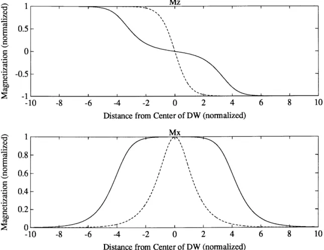
Mz for domain wall in a cubic material with magnetostriction Mx for domain wall in a cubic material with magnetostriction Mz for domain wall with "magnetostatic anisotropy"
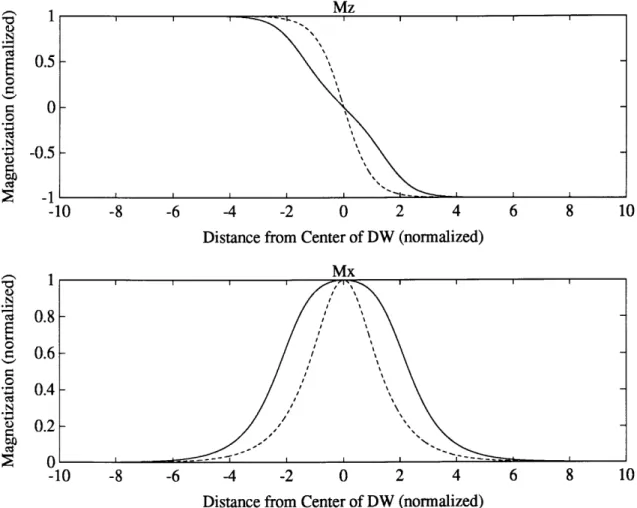
Mx for domain wall with "magnetostatic anisotropy"
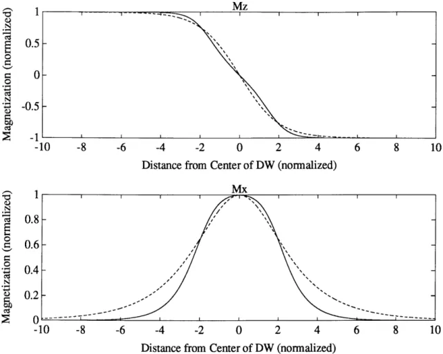
Mz for domain wall with adjusted "magnetostatic anisotropy" Mx for domain wall with adjusted "magnetostatic anisotropy"
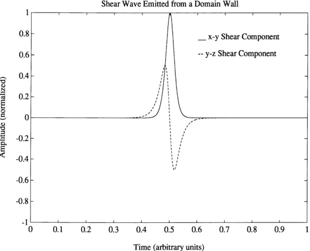
Coordinate system used for the moving domain wall Shear components of elastic radiation
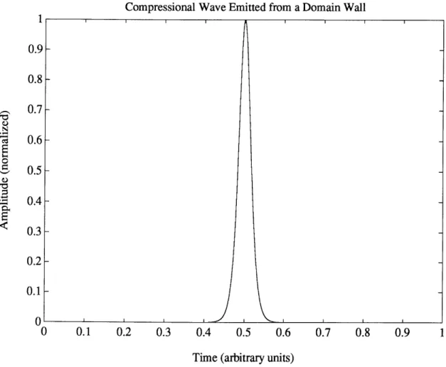
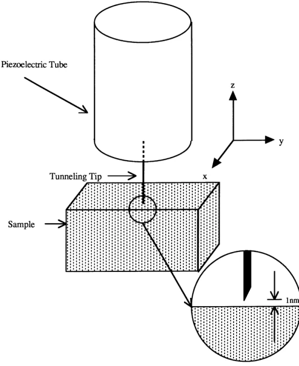
Longitudinal component of elastic radiation Piezoelectric tube and tunneling tip
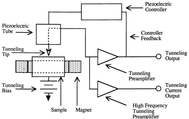
Block diagram of standard scanning tunneling microscope Modifications to standard scanning tunneling microscope Block diagram of standard tunneling head
Block diagram of modified tunneling head
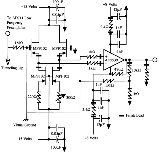
High frequency inverting current to voltage converting amplifier Frequency response of current to voltage converter
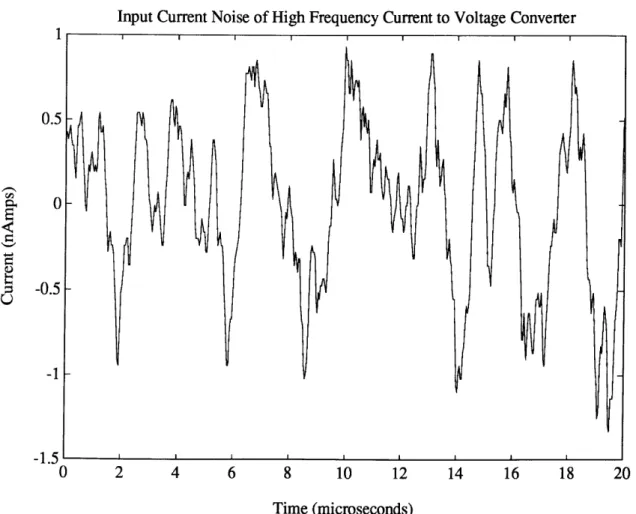
Input current noise of the current to voltage converter Longitudinal surface deflection near tunneling tip
26 26 26 29 33 44 44 53 53 54 54 79 96 97 106 107 108 110 110 111 112 113 115
Figure V.9 Figure V.10 Figure V.11 Figure VI. 1 Figure VI.2 Figure VI.3 Figure VI.4 Figure VI.5a. Figure VI.5b Figure VI.6 Figure VI.7 Figure VI.8a, Figure VI.8b Figure VI.9 Figure VI.10 Figure VI. 11 Figure VI.12 Figure VI.13 Figure VI.14 Figure VI. 15 Figure VI. 16 Figure Figure VI.17 VI.18 Figure VI.19 Figure VI.20
Shear surface deflection near tunneling tip on rough surface Measurement of shear wave near tunneling tip
Small traveling shear wave near tunneling tip [100] easy axis single crystal picture frame [111] easy axis single crystal picture frame 180 domain wall motion in picture frame
Photomicrograph of domain structure in picture frame Photomicrograph of "tree" domains
Drawing of "tree" domain and surface poling
Picture frame cross-section for velocity measurements Source and sense coil configuration
Domain wall velocity versus time for 3.5 Oe applied field Domain wall velocity versus time for 0.5 Oe applied field Domain wall velocity versus time for interrupted applied field Domain wall velocity versus applied magnetic field
Front and side views of tunneling fixture Copper shield configuration on picture frame Pulse current source to drive source coil Tunneling tip placement for transverse waves
Measurement points for tunneling and atomic force microscope Surface plot of picture frame for an applied field of different frequencies
Cross-section of surface plot for 2Hz, 2.4 Oe sinusoidal field Surface plot of picture frame for different magnitude 5Hz applied field
Cross-section of surface plot for 5Hz, 4.7 Oe sinusoidal field Peak to Peak surface displacement versus applied field
116 117 117 119 120 121 123 124 125 127 127 129 129 131 132 134 135 136 137 139 140 141 142 143 144
Figure Figure Figure VI.21a VI.21b VI.22a Figure VI.22b Figure VI.23a Figure VI.23b Figure VI.24a Figure VI.24b
Sense coil response to a 5.8 Oe field pulse
Tunneling current response to a 5.8 Oe field pulse Effective surface displacement for a 5.80e field pulse with lOnA tunneling current: Averaged
Effective surface displacement for a 5.80e field pulse
with lOnA tunneling current: Electrostatic coupling cancellation Effective surface displacement for a 5.80e field pulse
with 20nA tunneling current: Averaged
Effective surface displacement for a 5.80e field pulse
with 20nA tunneling current: Electrostatic coupling cancellation Effective surface displacement for a 5.80e field pulse
with 40nA tunneling current: Averaged
Effective surface displacement for a 5.80e field pulse
with 4OnA tunneling current: Electrostatic coupling cancellation 149 149 150 150 151 151 152 152
List of Tables
11 Acknowledgement
I wish to thank all the people who have contributed directly and indirectly to this thesis. There are many members of the M.I.T. community who have donated their time and equipment to enable its completion.
I would like to thank: David Robinson in the undergraduate physics laboratories for all his help over the past years. The members of the Uhlig Corrosion Laboratory for all the tid bits borrowed. The members of the graduate physics office, and especially Peggy Berkovitz for all her help. Dr. Robert O'Handely, of the Material Science and Engineering Department for helping to initiate my interest in magnetism and then supplementing my education and reading parts of the theoretical background for this thesis.
I wish to acknowledge the help of the magnetics community in assisting this research. Especially I'd like to thank: Mr. Jim Salsgiver of Allegheny Ludlum Corp. for helping me find the samples for experimentation. Dr. Robert Krause of Magnetic
International for the SiFe picture frame single crystal used to test the theoretical model and the tunneling transducer.
I would like to thank the past and present members of the Specialty Material Laboratory at M.I.T. including: Louise Harrigan for all her help. My colleagues, Ron Gans and Mira Misra for their interest and contributions to my research and their friendship during the day to day existence at M.I.T. Dr. Bruce Jette for the challenge to keep up with him, and the technical assistance offered whenever I needed it. Dr. James Bellingham, who has been my friend and peer for almost all my years at M.I.T. Professor Margaret L.A. MacVicar for her constant support and dedication to me as a scientist. I wish that she was here to see the finished product.
I'd like to thank Leslie Lawrence for her unwavering dedication to Professor MacVicar's students. All of us feel that she is one of the most special people we have had the pleasure of working with. I would like to thank Dr. Kevin Rhoads for his technical assistance and friendship. His constant reassurance and advice allowed me to bring my work to a level I never thought I could reach. Thanks to all the other people working for Professor Robert Rose who were always willing to help. Professor Robert Rose for his guidance and support through the hard years of this thesis. It is no wonder that Professor MacVicar left us in his hands. There are none better at M.I.T.
Finally I would like to thank my family: To my father for permitting me to use his facility at the Advanced Materials Laboratory, and his assistance throughout my years at M.I.T. Thanks to my son Joshua for showing me what is important in life. And most of all my wonderful wife Kara, she has supported me with love throughout. She has made this thesis work tolerable. I could not have done it without her.
Chapter I: Introduction 1.1 Background
A ferromagnetic material emits elastic radiation during the magnetization process. This type of emission was first theoretically proposed and subsequently measured by Lord [1967 and 1975] and Lord et al. [1974]. Elastic radiation is a traveling stress wave propagating in an elastic medium. In general, emission of elastic radiation in any
material, termed an acoustic emission because the frequency is typically in the audible or ultrasonic range, is directly related to sudden changes in the internal strain distribution of the material [Maldn and Bolin 1974]. Many possible sources of elastic radiation exist in materials, e.g., dislocation motion [James and Carpenter 1971], and growth of cracks in brittle materials [Evans and Linzer 1977]. For each of these possible sources there is a local change in the internal strain field, and stress field, which emits the elastic radiation. In a magnetic material a number of possible sources of elastic radiation exist [Higgins and Carpenter 1978, Ono 1986, Jiles 1988, and Guyot and Cagan 1991]. Magnetic sources of acoustic emission are discussed in this thesis with emphasis on the emission in the initial stages of magnetization, when domain wall motion is the dominant mechanism for the magnetization process.
1.2 Magnetoacoustic Emission: Background
Lord [1967] initiated interest in acoustic emission from ferromagnetic materials during magnetization with his theoretical investigation of elastic radiation from an oscillating 1800 domain wall. This theory is based on a planar 180 domain wall, a region separating two magnetic domains in which the magnetization rotates through an angle of 1800, whose amplitude modulates sinusoidally, while the wall remains spatially stationary. This is really a dynamic model for creation/annihilation because of the temporal modulation of the domain wall amplitude. Lord theorized that an oscillating, or
in his case a modulating, magnetic domain wall is a source of elastic radiation because of the changing strain field during the oscillations. The local strain field undergoes
oscillations caused by a magnetoelastic coupling of the domain wall to the crystal lattice. Lord et al. [1974] extended the theory, qualitatively, to include experimentally observed acoustic emission, referred to as magnetoacoustic emission when arising from magnetoelastic sources [Jiles 1988 and 1991], during magnetization of nickel. These later measurements were made such that isolation of elastic radiation from a unique source was not possible. The material geometry and microstructure did not permit the determination of the emission source. They concluded that since the magnetization changes discontinuously in a changing external applied magnetic field (this behavior is called the magnetic Barkhausen effect) the accompanying magnetoacoustic emissions can be attributed to the same discontinuous domain wall motion that is responsible for the Barkhausen effect.
1.3 Magnetoacoustic Emission: Models for Emission
Subsequent investigations of elastic radiation produced during magnetization of ferromagnetic materials have resulted in a number of emission models. None of these emission models accurately describe all the phenomena associated with magnetoacoustic emission. The main similarity among almost all models is that they disregard 180 domain walls as sources of magnetoacoustic emission.
I.3a Magnetoacoustic Emission: Magnetoelastic Energy Model
The most commonly used models are based on the work of Kusanagi et al. [1979a] which utilizes the conclusion by Lord et al. [1974] that magnetoacoustic emission during magnetization is caused by discontinuous domain wall motion. Kusanagi et al. attempt to determine the net change in total elastic energy, AEei, from a
combination of magnetoelastic and elastic strain energy densities of the material before and after the discontinuous motion of a domain wall. The dynamics of domain wall motion are not included, only the net change in the magnetization is used. They postulate that at least some of the net change in total elastic energy is emitted as elastic radiation. Kusanagi et al. propose that only non- 180 domain walls, a region separating two
magnetic domains in which the magnetization rotates through an angle less than 1800, can contribute to the magnetoacoustic emission. This is because there is a negative net
change in the total elastic energy of a magnetic material after non- 180* domain wall motion in a material with cubic magnetocrystalline anisotropy, where as there is no net change in the total elastic energy for 180 domain wall motion. Kusanagi et al. have made a number of incorrect assumptions in their calculation. This work is discussed in Chapter III.2a.
Further evidence for the dismissal of 1800 domain wall motion as a possible source of magnetoacoustic emission is a comparison of the intensity of elastic radiation from material with cubic magnetocrystalline anisotropy, which contain many non- 180* domain walls, and uniaxial magnetocrystalline anisotropy, which contain very few non-1800 domain walls. In cobalt (uniaxial), Kusanagi et al. [1979a] measure lower levels of magnetoacoustic emission than those in iron (cubic). Since there are far fewer non-180* domain walls in cobalt, they postulate that non- 180 domain walls must be the source of magnetoacoustic emissions. The relative difference in the magnetoacoustic emission for cobalt and iron or nickel is not presented by Kusanagi et al. Their general conclusion, which is widely accepted, is that 180 domain walls cannot play a role in magnetoacoustic emission observed during magnetization.
In addition to the type of domain wall responsible for magnetoacoustic emission in magnetic materials, Kusanagi et al. [1979a] list a number of other predictions by their model. These include:
1) The intensity of the magnetoacoustic emissions should be related to the
magnetoelastic constants and the number of energy emission sites n(H), where H is the applied magnetic field.
2) The intensity of magnetoacoustic emission should depend on both applied stress and residual stress since n(H) is dependent on these stresses.
3) The intensity of magnetoacoustic emission should depend on internal strains. It is the relation between applied stress, internal strain and the intensity of
magnetoacoustic emission that can be tested experimentally.
I.3b Magnetoacoustic Emission: Effects of Applied Stress and Internal Strain The effects of stress on magnetoacoustic emission are reported by Kusanagi et al. [1979a and 1979b]. It was observed that, in general, increased applied stress, either tensile or compression, causes a decrease in the amplitude of the magnetoacoustic
emission. Kusanagi et al. did report a maximum, or two maxima in the case of nickel, in the region close to, but not exactly at, the zero load point. Their general results have been verified by a number of authors [Ono and Shibata 1980 and 1981, Shibata and Ono 1981, Burkhardt et al. 1982, Kwan 1983, Ono 1986, Buttle et al. 1986, Edwards and Palmer 1987, Kim and Kim 1989, Namkung et al. 1989 and 1991, and Ng et al. 1992a]. Edwards and Palmer determined that some of the rapid decrease in magnetoacoustic emission could be caused by the experimental setup used to apply the external stress. The relative degree of clamping during application of the applied stress can alter the fundamental resonance frequency and the magnitude of resonance, thus altering the magnetoacoustic emission measured by a piezoelectric transducer. More recently Ng et al. have measured an increase in the magnetoacoustic emission for nickel, under tension, for applied magnetic fields both parallel and orthogonal to the applied stress.
The observed dependence of the intensity of magnetoacoustic emission on applied stress is explained using magnetoelastic energy [Jiles 1991, Kwan 1983, Edwards and
Palmer 1987, and Ng et al. 1992a]. For materials with positive magnetostriction the ratio of 180 to non- 180" domain walls increases when that material is under tension. Thus the magnetoacoustic emission should decrease. Likewise for materials with negative magnetostriction the ratio of 180* to non-180* domain walls decreases when that material is under tension. So here the magnetoacoustic emission should increase (possibly the increase observed by Ng et al. [1992a]). More troubling is the effect compressive stress should have on the magnetoacoustic emission using this type of explanation. In this case, the change in non-180 domain walls is opposite to the case during tension, and thus the intensity of magnetoacoustic emission of a material under compression should change accordingly. This is not observed [Jiles 1991, Kusanagi 1979a, Ono and Shibata 1981, Burkhardt et al. 1982, Ono 1986]. The dependence of magnetoacoustic emission on applied stress is more complicated than a simple change in the relative area of non-180 to non-1800 domain walls. In a dynamic model of magnetoacoustic emission, the effects of the applied stress on the actual motion of domain walls is also critical. Inclusion of domain wall motion is suggested by Namkung et al [1989 and 1991] for materials under uniaxial stress.
The response of magnetoacoustic emission in materials under biaxial stress has also been investigated [Buttle et al. 1990, and Ng et al. 1992b]. In a cross shaped steel specimen, Buttle et al. report that the intensity of magnetoacoustic emission does not appear to depend directly on the level of tensile stress applied orthogonally to the applied magnetic field. This is inconsistent with a model in which non- 180* domain walls are the unique source of magnetoacoustic emission at low magnetic fields. The opposite result is observed by Ng et al. [1992b]. In a cross shaped nickel specimen, in which the majority of domain walls are non-180* domain walls (actually either 71* or 1090), they report a strong dependence of magnetoacoustic emission on the level of applied stress. The difference could stem from the existence of different dominant magnetoacoustic emission mechanism in these materials with very different domain wall configurations.
The dependence of magnetoacoustic emission on internal strain is also
contradictory to that hypothesized by Kusanagi et al. [1979a]. It has been determined that cold working, increasing internal strain, causes a decrease in the intensity of magnetoacoustic emission [Ono and Shibata 1981, Kwan 1983, Ono 1986, and Buttle
1986 and 1987]. On the other hand the same studies indicate that annealing increased the intensity of magnetoacoustic emission. This is inconsistent with the concept that the intensity of magnetoacoustic emission is directly proportional to the internal strain, and likewise inconsistent with the concept that the increased number of active emitting sites occurs with increased internal strain. As is shown in Chapter III.2a, Kusanagi et al. have incorrectly accounted for the internal strain. The corrected model suggests that the
change in total elastic energy is not directly dependent on internal strain. If the volume of material involved at each individual site is increased with decreased strain, the increase in the intensity of magnetoacoustic emission upon annealing can be accounted for.
I.3c Magnetoacoustic Emission: Dynamic Inelastic Strain Model
In order to deal with the direct problems associated with the model proposed by Kusanagi et al. [1979a], Ono and Shibata [1981] have attempted to look at the emission of the elastic radiation from a dynamic point of view. This model uses an approach formulated by Maldn and Bolin [1974] and Ono [1978] for acoustic emission by a moving dislocation where the equations of motion for a linear elastic media are solved after introducing an inelastic strain associated with the dislocation. Maldn and Bolin determine that for a step change in inelastic strain, Ae*, the amplitude of elastic radiation emitted should be proportional to Ae* and the volume associated with the change. Ono and Shibata employ this dynamic model for the motion of the non- 180 domain wall. They again conclude that since there is no net static Ae* after motion of a 180 domain wall, there can be no magnetoacoustic emission from 180 domain wall. Such a
conclusion ignores any possible dynamic changes in the strain field within the 1800 domain wall. This model does not specifically give information about the magnitude or functionality of the change in inelastic strain. Thus the observed effects of applied stress and residual strain can not be directly addressed.
I.3d Magnetoacoustic Emission: Creation/Annihilation Model
The model of Ono and Shibata [1981] suggests a direct relation between the Ae* and the saturation magnetostriction constants, Xs. Kwan [1983] and Kwan et al.[1984] conclude that depending on the type of material, and the dominant mechanisms for magnetization, the level of magnetoacoustic emission should be linear with saturation magnetostriction )s, in a moderate applied magnetic field. Kwan and Kwan et al. observe a linearity in nickel based alloys used in these experiments, but not in iron based alloys.
Such a relation was not observed by Guyot et al. [1990a, 1990b and 1991]. In the experiments performed by Guyot et al., yttrium iron garnet based ferrimagnetic compounds were investigated. Significant amounts of magnetoacoustic emission is reported even for a polycrystalline material with manganese substitution such that the
saturation magnetostriction constant is zero. Guyot et al. propose that domain wall motion models cannot account for the observed emission from this material. In addition, they point out that the shape demagnetizing effect of the sample can significantly alter the magnetoacoustic emission. Guyot et al. [1987, 1988, 1990a, 1990b and 1991] find a direct proportionality between magnetoacoustic emission and hysteresis loss in the ferrite, amorphous and mu-metal samples. Thus Guyot et al. propose that a domain wall
annihilation/creation mechanism is more appropriate as a source of magnetoacoustic emission.
Although a domain wall creation/annihilation mechanism cannot be discounted as a contributor to the magnetoacoustic emission, the conclusion that the magnetostriction coefficient does not play a role is not proven. Guyot et al. [1990a, 1990b and 1991] discount the lack of magnetoacoustic emission seen by Kwan [1983] and Kwan et al. [1984] for certain nickel-iron alloys, where X100, X111 and the saturation magnetostriction coefficient, Xs, are all zero, as an artifact of other magnetic parameters. On the other hand Guyot et al. use Y3Fe4.92Mno.080 12 with a zero Xs, but non-zero X100 and X1 11 [Dionne and Goodenough 1972]. It is unknown whether the value of ks is determined using the standard formula for an anisotropic material [Jiles 1991] or the corrected formula for polycrystalline aggregates [Callen and Goldberg 1965]. If a model for magnetoacoustic emission includes a term dependent on individual magnetostriction constants, then magnetoacoustic emission for the ferrite tested by Guyot et al. should be finite, as was found. The determination that magnetostriction does not play any role in emission of elastic radiation in a ferromagnet during magnetization is not proven by Guyot et al.
Another domain wall creation/annihilation has been proposed by Kim and Kim [1989]. This model couples the creation/annihilation of the domain wall to
magnetoacoustic emission via the magnetostriction. Although the premise of the argument is not inaccurate, the method for determination of the strain field is incorrect (this is discussed in Chapter III). Thus the results of this model cannot be accepted.
I.3e Magnetoacoustic Emission: 1800 Domain Wall Model
Many proposed mechanisms exist for magnetoacoustic emission in a
ferromagnetic material. Other than early work by Lord [1967 and 1975], Lord et al. [1974] and Burkhardt, et al. [1982] and a more recent review by Kuleev et al. [1986], the possibility that 180* domain wall motion is a source of emission has been discounted.
20 Such a conclusion is based on a non-dynamic and non-realistic model of the
magnetization process. A true dynamic model must include the emission by 180 domain wall motion, along with non-180" domain wall motion and domain wall
creation/annihilation.
Experimental evidence suggest that 180" domain walls can cause measurable magnetoacoustic emission in single crystal silicon-iron. Kwan [1983] observed significant magnetoacoustic emission in a single crystal. She suggested that the source might be 1800 domain walls. But later, in order to demonstrate that the observed
magnetoacoustic emission from a single crystal is consistent with her proposal of a direct relation between the intensity of magnetoacoustic emission and saturation
magnetostriction, she concludes that this is unlikely. Gorkunov et al. [1986] also measured large magnetoacoustic emission in silicon-iron oriented in the [100] direction. They observed reasonable correlation between the Barkhausen effect and
magnetoacoustic emission at the early stages of magnetization. Since the majority of Barkhausen jumps at this stage of magnetization are caused by 180' domain walls, especially in their particular single crystal orientation, they concluded that the motion of 180" domain walls must be related directly to the motion of non-180" domain walls. This conclusion was drawn to overcome their difficulty in explaining how 180" domain walls could be a magnetoacoustic emission source. The claim that the 180 domain walls drag the non-1800 domain walls along in the early stages of magnetization is also suggested by Namkung et al. [1991].
1.4 Scope of Thesis
This thesis extends the original calculations by Lord [1967] and Kuleev et al. [1986] to a model in which a spatially moving 180 domain wall emits elastic radiation in a ferromagnetic material. This model shows that it is the local change in the
domain wall. It is this change in the magnetization distribution within the domain wall, which is required for motion [Landau and Lifshitz 1935, and O'Dell 1981], that produces the magnetoacoustic emission from the 180 domain wall. The model proposed in this thesis, in which the acceleration of a 180* domain wall is a source of elastic radiation, can then be added to the list of mechanisms for magnetoacoustic emission.
In order to model the elastic radiation emitted from 180* domain wall motion, the magnetization within the domain wall is needed. Chapter II discusses models of a static 180 domain wall in the cubic material. The cubic material is chosen since attempts at experimental verification are performed on a cubic 3% SiFe single crystal. A number of inconsistencies found in the literature describing the 180 domain wall are discussed.
Chapter III is a review of the current models and descriptions of magnetoacoustic emission. This is background for Chapter IV, in which the static domain wall model developed in Chapter II is extended to a simple dynamic model for the 180 domain wall. A model for the magnetization distribution within a moving domain wall is presented. The basis of the model follows the presentation of O'Dell [1981], but extends his postulates to determine a self consistent solution to the Landau and Lifshitz equation of motion including Gilbert damping [Gilbert 1955]. The magnetization distribution derived in this thesis is shown in Appendix C to be a lower energy state than that of the Walker
solution commonly used [Dillon 1963 and Schryer and Walker 1974]. The magnetization distribution is used to find the elastic interaction of the moving domain wall with the magnetic crystal. This interaction produces magnetoacoustic emission if the domain wall is accelerating.
The model presented follows the approach used by Lord [1967] and Kuleev et al. [1986]. This literature is based on a number of assumptions about the symmetry of the magnetic system and the elastic displacement vectors which are only approximate for magnetic materials containing domain walls. Both papers are based on the premise that the stress tensor is symmetric and that the rotation tensor plays no role in the magnetic
system. As pointed out by Auld [1968] and Brown [1965 and 1966], these are two of a number of incorrect assumptions commonly made when dealing with deformable
ferromagnetic materials. Auld specifically deals with the elastic effects in ferrimagnetic materials undergoing electron spin resonance, but does not deal with domain walls.
Since a corrected formalism has not been attempted when modeling the dynamics of the domain wall, the accuracy of the model presented in this thesis is only
approximate. But the model is of value because it introduces a clear conceptual basis for the elastic coupling of a 180 domain wall to the magnetic material which produces magnetoacoustic emission. The corrections required to accurately model the
magnetoelastic coupling at the domain wall do not invalidate the conclusion made in this thesis using the simpler model that there is magnetoacoustic emission from 180 domain walls.
Experimental techniques for the measurement of magnetoacoustic emission are discussed Chapter V. The standard techniques are presented. Next the design of a high frequency tunneling acoustic emission transducer developed for this thesis is discussed. The tunneling transducer has high sensitivity to local surface motion. The transducer can detect surface motion of approximately 0.5A at a bandwidth of greater than 5MHz before any signal processing or averaging. This sensitivity can be used with material geometries to attempt to isolate magnetoacoustic emission from 1800 domain walls.
Using the tunneling transducer, the validity of the prediction that a 180 domain wall can be the source of magnetoacoustic emission is then tested experimentally by measurement of magnetoacoustic emission in an imperfect picture-frame single crystal of iron with 3% silicon. If the picture frame is perfect, the geometry isolates 180* domain walls allowing isolation of emission from other possible sources. Since the crystal is
slightly out of alignment a more complex domain structure exists which can obfuscate the experimental results. The results of experimentation on SiFe presented in Chapter IV
23 indicate that any emission in the crystal is below limit of detection of the tunneling
transducer.
In Chapter VII the consequences of the model and the experimental results are discussed along with a presentation of future experiments that should circumvent the experimental difficulties encountered in this thesis. These experiments are designed to enhance the understanding of magnetoacoustic emission in ferromagnetic materials.
24 Chapter II: Magnetic Domain Walls
11.1 Introduction
An investigation of the elastic interaction of a moving 180 Bloch wall in a
ferromagnetic material requires, as a foundation, a theoretical description of a static Bloch wall. The Bloch wall is referred to simply as a domain wall; all other types of
interdomain regions are referred to by using specific names. The theoretical aspects of this thesis employ domain wall theory, published by Landau and Lifshitz [1935], which models the statics and dynamics of magnetization in a material, using the Landau-Lifshitz equation. The Landau-Lifshitz equation can be used to determine both the static and dynamic structure of a domain wall. The use of the Landau-Lifshitz equation is discussed in greater depth in Chapter IV of this thesis.
The approach used here to model characteristics of domain walls is similar to that of O'Dell [1981]. O'Dell's postulate is expanded upon and compared to the Walker solutions to the Landau and Lifshitz equation [Dillon 1963 and Schryer and Walker 1974]. Although it is easier to determine the thickness of and magnetization distribution in a domain wall using an energy argument, by using the Landau and Lifshitz approach the dynamic characteristic of the domain wall can be found. The Landau-Lifshitz
equation is needed to develop a model for the magnetization distribution within a domain wall to be employed in the modeling of emission of elastic radiation caused by the motion of a 180 domain wall. Thus the groundwork for the later calculations should be
presented in this formalism.
This chapter presents the description of a 180* domain wall used in the model for magnetoacoustic emission. The appropriate magnetization distribution is determined for this domain wall. The magnetization distribution is found using a classical continuum approximation to the magnetic system. In addition, some of the fundamentals of domain wall theory are presented. This is done to elucidate a number of approximations and
assumptions made by earlier authors that are not valid. The result of these
approximations and assumptions does not significantly alter the accepted structure of the domain wall [Landau and Lifshitz 1935, Kittel 1949, O'Dell 1981, and Chikazumi
1986], but does change the interpretation of the cause of the 180* domain wall in cubic materials.
11.2 Overview
The defining characteristic of a 180* domain wall is that, when static, there is no component of magnetization normal to the wall. Instead the magnetization rotates entirely within the plane of the wall (tangential to the wall). Such a domain wall configuration is experimentally observed in materials with either cubic or uniaxial magnetocrystalline anisotropy. In this thesis a material is considered as having cubic magnetocrystalline anisotropy if it has cubic crystal symmetry and thus magnetocrystalline anisotropy energy which has cubic symmetry (i.e. iron, which has body centered cubic symmetry). A material is considered to have uniaxial magnetocrystalline anisotropy if it does not have cubic crystal symmetry and thus the magnetocrystalline anisotropy energy has only one easy axis (i.e. cobalt, which has hexagonal crystal symmetry) [Chikazumi 1986]. Although cubic material is the focal point of this thesis the theoretical parts of this work also include some discussion of uniaxial material.
Lifshitz [1944] first pointed out that the energy terms needed to form a 180* domain wall in a cubic material differ from those required for a uniaxial case. A 180' domain wall in a uniaxial material can be derived with only exchange and
magnetocrystalline anisotropy terms. This is not the case for the cubic crystal. The difference stems from the fact that, since cubic material has six easy, orthogonal directions, a rotation of the magnetization from an easy direction through 90* can leave the magnetization pointing in a different easy direction. The uniaxial system has only two easy directions 180 apart, so the anisotropy energy is lowest when the magnetization is
26 in either of the two easy directions. Uniaxial material has only one dominant domain wall configuration, the 180 domain wall, if only magnetocrystalline anisotropy energy is considered. In the cubic material the magnetocrystalline anisotropy permits the
formation of either 90* or 1800 domain walls. If the same approach is used to calculate the domain wall structure of cubic material, assuming an infinite, perfect crystal, as is used for the uniaxial case, the 180" domain wall is not a consistent solution to the Landau-Lifshitz equation. The only achievable solution is a 90* domain wall, with no magnetization normal to the domain wall. Such a wall is referred to as a tangential 90* domain wall. The configuration of magnetization in the vicinity of three types of domain walls is shown in Figure II.la-c.
Domain Wall
Figure la) Figure 1b) Figure 1c)
Figures II. 1a-c. The direction of magnetization (marked by the arrow) on either side of a domain wall. la) The 180* domain wall with magnetization rotation in the plane of the wall. 1b) The tangential 90* domain wall with magnetization rotation in the plane of the wall. 1c) The normal 90* domain wall with a component of magnetization normal to the plane of the wall.
Observations of real cubic materials have found both tangential 180 domain walls and normal 90* domain walls [Chikazumi 1986, Kittel 1949, and Kittel and Galt 1956]. The observed static normal 900 domain wall has a component of magnetization normal to the domain wall, while the observed static 180* domain wall does not have a component
of magnetization normal to the wall. It is not immediately apparent why both tangential
900 and 1800 domain walls should not exist. Details of this are presented in this chapter.
H.3 The Static Domain Wall Equilibrium Equation
A static domain wall can be modeled as an equilibrium between the total magnetic field and the magnetization of a material on a point by point basis. This method for determining the magnetic characteristics of a material is the basis of micromagnetics, first developed by Brown [1963]. The equilibrium condition is given by the Landau-Lifshitz equation for the static case,
Mx H =0, (11.1)
where appropriate magnetization M and magnetic field H for the system investigated in this thesis are given later in this chapter. Equation (11.1) states that the magnetic torque at any point in a medium in equilibrium must be zero. If all the appropriate contributions to the magnetic field are included in H, the magnetization of the medium is described by the solution of equation (11.1). An analytic solution seldom exists without approximation to the magnetic field terms. This is typically done to permit determination of the
approximate magnetization distribution within the domain wall.
The standard calculation of the structure of the domain wall is to minimize
energies by balancing magnetic exchange and magnetocrystalline anisotropy [Landau and Lifshitz 1935]. This approach does not use the Landau-Lifshitz equation directly. A more accurate picture must account for six magnetic energies, or when using the Landau-Lifshitz equations, the corresponding six magnetic field terms, which influence the magnetic domain wall. These fields, in addition to the two already named, are the magnetostatic self field, the magnetoelastic field, magnetic surface anisotropy, and the externally applied field [Kittel 1949, Kittel and Galt 1956, Maugin 1979, O'Dell 1981 and Scheinfein et al. 1991]. Surface anisotropy is ignored throughout this thesis.
28 The magnetic field terms, except the externally applied field, are typically
presented in terms of magnetic energies. Each magnetic field term, Hk, is related to the appropriate magnetic energy term as follows,
Ek=-M -Hk (11.2)
In a ferromagnetic material the magnetic field terms, Hk, can be determined from each magnetic energy term:
Hk =- k ) i, (11.3)
where Ek is expressed in cartesian coordinates, M, is the saturation magnetization, and
(Xi CX, (X3) are the three direction cosines in the coordinate system. Equation (11.3) is valid only under the approximation that the magnetic material is rigid (no magnetic strains are permitted). In a deformable medium an additional term is present in equation (11.3) [How et al. 1989, Maugin and Miled 1986, and Motigi and Maugin 1984a and 1984b]. Appendix A describes three of the magnetic energy contributions: exchange energy, magnetocrystalline anisotropy energy, and magnetoelastic energy. The applied magnetic field, normally taken to be zero for the static wall, comes into the Landau-Lifshitz equation directly and will not be needed until domain wall dynamics is discussed in Chapter IV.
11.4 The Static Domain Wall
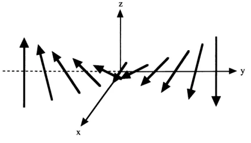
The domain wall is modeled as a transition layer which separates two large (compared to the domain wall) uniformly magnetized regions. The simplest model, which will be used throughout this thesis is that of an infinite material with a central x-z planar domain wall (Figure 11.2). The normal to the domain wall is in the y-direction. The magnetization is Ms, taken to be in the positive z-direction at y = -oo and in the
negative z-direction at y = + oo. The consequences of choosing these conditions at + oo
will be discussed later in this chapter. The magnetization, M, in the static domain wall is assumed to rotate smoothly (a continuum model) only in the x-z plane from -z to +z. The continuum approximation is used to simplify the modeling of the domain wall. The dominant energy contributions in reality come from quantum mechanical spin-spin and spin-orbit interactions. But since the domain wall extends of a large number of lattice sites, these interactions can be approximated by continuous classical energy expression even though their source is purely quantum mechanical (see Appendix A).
z
--- ---- --- --- -y
x
Figure 11.2 The region of magnetization rotation, where M switches from + Ms to -M, is the domain wall. Arrows represent the magnetization vector.
The magnetization is given by Mx = M, sinO and Mz = M, cosO. There are a number of domain wall and material geometries for which there is a component of the magnetization in the normal direction to the static domain wall: i.e. the Ndel wall
[Malozemoff and Slonczewski 1979], at a surface where the domain wall terminates [Krinchik and Benidze 1974, Scheinfein et al. 1989 and 1991], at a closure domain
30 [Kittel 1949, and Kittel and Galt 1956]. These types of domain walls will not be dealt with in detail in this thesis.
II.4a The Static Domain Wall: Magnetic Field Terms
Three magnetic field terms needed to calculate the static equilibrium of the magnetization configuration, and thus domain wall structure in an infinite rigid material, can be determined using equation (11.3) and the energy terms from Appendix A. These are magnetic exchange, magnetocrystalline anisotropy and magnetostatic self energies. The magnetic exchange energy for material with cubic crystal symmetry is
Eex 2A M. V2M, (11.4)
where A is the exchange constant (this is considered a material constant) [O'Dell 1981]. This expression is a classical continuum approximation of the quantum mechanical
exchange interaction which cause ferromagnetism. The exchange constant for each of the three types of cubic crystal structures is the same to within a constant which is dependent on the number and configuration of nearest neighbors to any particular atom. This expression for magnetic exchange energy is discussed in Appendix A. It should be noted that this expression and the more typical expression for exchange energy in a continuous medium are equivalent [Chikazumi 1986 and Kittel 1949]. The choice of this expression is made for convenience when applying the dynamic equations for the magnetization.
From the exchange energy given above the exchange field can be calculated:
H 2A V2M. (11.5)
Although the exchange field for a non-cubic crystal structure differs from that of the cubic crystal structure, the general form of the exchange field for the hexagonal crystal structure (the only non-cubic being used in this thesis) is the same as (11.5), only with a different exchange constant for each direction [Landau and Lifshitz 1982].
The magnetocrystalline anisotropy field is the second term needed to determine the structure of the domain wall. This energy can be written as a classical continuum approximation to a quantum mechanical spin-orbit interaction. Here there are significant differences between expressions for the fields of the cubic crystal and no-cubic crystal symmetries. For a cubic material the magnetocrystalline anisotropy energy to lowest (non-constant) order in the magnetization is given by
Ea= K,
[a
2 aj2], (11.6)where Ki is the magnetocrystalline anisotropy constant, (ai, a2, a3) are the direction
cosines between the actual and easy directions of magnetization, and i +
j.
A material with this type of magnetocrystalline anisotropy is called a cubic material in this thesis. For a material with non-cubic crystal symmetry the lowest (non-constant) order term in the magnetocrystalline anisotropy energy is given byEan= Kui [(X12 + X2 21, (11.7)
where Kui is the uniaxial magnetocrystalline anisotropy constant and (ai, a2) are direction cosines between the actual and the easy directions of magnetization, which in this case is in the 3-direction. A material with this type of magnetocrystalline anisotropy is referred to as a uniaxial material in this thesis.
From these energy terms the anisotropy fields can be calculated using equation (11.3). They are, assuming the wall geometry depicted in Figure 11.2,
Ha= - 1 VK 2 aj2]i, (11.8)
for cubic (i is the unit vector in i-direction) and
H -2 Kui [ aix +a 2 y], (I9
for uniaxial (x and y are the unit vectors in the x- and y-directions respectively). In both these cases the anisotropy field is zero if magnetization is in an easy direction. It is typical to write the anisotropy field such that it is parallel to the easy direction in a uniaxial material [Chikazumi 1986, Jiles 1991]. But as pointed out by Landau and Lifshitz
[1935] and O'Dell [1981], the representation with the anisotropy field orthogonal to an
easy axis is equivalent to within a scalar constant. This representation, with Ha orthogonal to an easy axis, is used by O'Dell.
The final energy term needed to determine the structure of the domain wall is the magnetostatic self energy. This energy is the most difficult to deal with because it is non-local. The expression for the magnetostatic self field can be found from the general form of the magnetic scalar potential to be
Hst= 1 V f M dV+f M -ndS, (1.10)
where rjk is the distance between the point of integration, i, and the point, k, where Hst is evaluated and n is the unit vector normal to the surface of integration [Jackson 1975, O'Dell 1981]. In the standard approach, when investigating domain walls, one attempts to choose a geometry, magnetization distribution, and surface conditions so as to
eliminate the magnetostatic self field, and thus simplify the model. Landau and Lifshitz
[1935] achieve this by closure domains and restrictions on the rotation of the direction of
magnetization within the domain wall. They then investigate the domain wall far from the closure domains. A discussion of this is presented below for the uniaxial material.
II.4b The Static Domain Wall: Closure Domains and the Infinite Crystal Landau and Lifshitz [1935] were the first to attempt an investigation of the domain structure in a finite uniaxial material by postulating the existence of closure domains at two of the surfaces of the material (Figure 1.3). The introduction of these closure domains is an attempt to minimize the magnetic energy of the crystal by
eliminating the free poles on the surface, Ma = 0, and forcing the div(M)= 0 inside the material. Their model covered uniaxial materials exclusively.
Closure Domain Normal to Surface
Figure 1.3 Example of closure domains at the surface of a magnetic material. The closure domains assure that M, = 0. The cross-sectional view is that of a surface Ndel wall of the form reported by Scheinfein et al. [1989 and 1991].
From this model Landau and Lifshitz [1935] were able to estimate domain structure within the material as a function of the size of the material. They showed that the width of the long domains are proportional to the square root of their length, w =
the closure domains in the uniaxial material have a large anisotropy energy, since they are magnetized in a hard direction. The domain wall configuration is a trade-off between the energy of the domain wall and the energy of the closure domains. The number of long domains and closure domains is determined by the size of the material.
This model was extended to cubic materials by Lifshitz [1944] who postulated the existence of cubic closure domains. The closure domains in cubic materials were
observed by Williams et al. [1949]. In the cubic material the closure domains are magnetized in an easy direction. Thus the closure domains are energetically favorable. Lifshitz determined that in cubic material the width of the long domains is again
proportional to the square root of their length, w = C21112, where C2 is a constant. But in this case it is magnetoelastic energy which limits the size of the closure domains relative to the long domains.
Lifshitz [1944] has determined that for large enough uniaxial materials a more complicated domain structure, with domain wall branching, can occur. He determined that in the uniaxial material Co, that this branch should occur as soon as the linear dimension is of the order of 10-5 cm. The branching is also a result of the large
anisotropy energy associated with the closure domains. This type of complicated domain structure is observed in uniaxial materials [Takata 1963 and Chikazumi 1986].
A thermodynamic investigation into the existence of closure domains is reported by Privorotskii [1971 and 1976]. He claims that in a uniaxial material it is
thermodynamically unstable to form closure domains of the form postulated by Landau and Lifshitz [1935]. Instead a more complicated branching structure similar to that suggested by Lifshitz [1944] and Takata [1963] must be present. In either case the magnetization distribution at the surface is such that the magnetic energy is minimized.
When the linear dimensions of the cubic material become large enough Lifshitz [1944] postulated that branching should occur in a similar manner to that predicted for
35
uniaxial materials. The magnetoelastic energy is the driving force for this branching. Such branch should not be observed experimentally in most real cubic materials because the relative size of the magnetoelastic energy is quite small. The predicted splitting
should occur in iron when the length of a single domain exceeds 104 cm.
So far the model does not look at the surface of the material orthogonal to the plane of the long domain wall (a surface parallel to the y-z plane in Figure 1.3). On this
surface there will be a normal component of magnetization unless the magnetization distribution in the domain wall is modified from that of the domain wall far from the
surface. Such a normal component has been measure in cubic materials [Krinchik and Benidze 1974] and predicted using a micromagnetic model by Scheinfein et al. [1989 and
1991] for both uniaxial and cubic materials. Scheinfein et al. [1989 and 1991] have demonstrated that the magnetization distribution undergoes a rearrangement at this surface to include a surface Ndel wall to act as a microclosure, see Figure 11.3. This
configuration permits Ma to remain zero at the surface, but results in a non-zero div(M). This contributes to the total magnetostatic self field in the magnetic material.
The infinite material approximation is used in modeling the domain wall in an attempt to ignore the effects of the magnetostatic self field. The success of such a model depends on what happens to closure and branching domains in the vicinity of the surfaces as well as the surface Ndel walls as the surfaces are extended to infinity. Using Landau and Lifshitz [1935] configuration for the uniaxial material and Lifshitz [1944] for the cubic material the closure domains would continue to exist, although their size would be dependent on the relationship w = Cil1/2. Even the branching domains located at the surface [Lifshitz 1944, Takata 1963 and Privorotskii 1971 and 1976] large would continue to exist as 1 approaches infinity. The same is true for the surface N6el walls, although their size does not change as that surface extends to infinity [Scheinfein 1989 and 1991 and Aharoni and Jakubovics 1991]. Thus in some materials it may be
acceptable to assume the different surfaces effects do not play a significant role in the domain wall configuration, but this is not assured. In fact the magnetostatic self field caused by the surface effects can be ignored in modeling the uniaxial material which is much thicker than the domain wall width [Scheinfein et al. 1989 and 1991]. But in the cubic material the effect of the surfaces, or more exactly the magnetostatic self field, are significant for finite materials as demonstrated by Scheinfein et al. [1989 and 1991]. As shown in this thesis this should also be the case for infinite materials.
11.4c The Static Domain Wall: Uniaxial Material
The domain wall structure for the uniaxial material is determined by the
micromagnetic equilibrium condition (1.1). It is appropriate to assume, for the uniaxial material, that the magnetostatic self field does not make a significant contribution to the structure of the domain wall. For an infinite material the surfaces shown in Figure 11.3 must be pushed to infinity. Doing this does not remove the surface domain structure [Landau and Lifshitz 1935] or the surface N6el walls. But in a large uniaxial material far from all surfaces, magnetostatic self field has little affect on the domain wall. The same can be concluded for the surface Nel walls. This is observed in the numerical models of Scheinfein et al. [1991] and Aharoni and Jakubovics [1991].
The magnetization distribution in the domain wall far from the closure domains and the surface Ndel walls can be found if it is assumed that My is zero (The only non-trivial term in (II. 1) is MxHz -MzHx = 0, where Mx and Mz are defined in Chapter 1.4). Hx and Hz can be found from the magnetic field expressions (11.5) and (11.9),
H =- 2Ku1 sin 0 + 2 A d (11.11)
MS MS dy2
and
where, since M is only dependent on y, the Laplacian becomes a second derivative with respect to y. Using the expressions for Mx, and My and 0 as the dependent variable, the equilibrium differential equation is determined to be
d20 -"! sin 0 cos 0 = 0.
(1.13) dy2 A
If the substitution dO/dy = u is made, the equation can be solved in terms of u(0). Since the magnetization is antiparallel at y = ±oo, dO/dy can be assumed to approach zero at ±oo. This forces the constant of integration to be zero and a simple first order differential equation can be found
S-=(Ku 1'~ /2 sin e. (1.14)
dy A
Solving this for y(O) yields
y = ( 1 2ln tan + C. (1.15)
Here C, the constant of integration, is zero since at y = 0, 0 = ± t/2. The general expressions for the magnetization as a function of y can be found from (11.15) to be
Mz = - MS tanh (), (II.16)
and
M_ =+ M sech A), (1.17)
where A is domain wall width parameter (A/Kui)1/2. The solution has both a positive and negative sign for the values of Mx. This is because the direction of rotation (clockwise or counterclockwise) relative to the normal direction to domain wall can not be
predetermined in this geometry. Either direction is equally energetically favorable, and both solutions are physically realizable.
II.4d The Static Domain Wall: Cubic Material
The static structure of the domain wall in an infinite cubic material will be calculated in the same manner as is presented in Chapter 11.4c. It is assumed that the closure domains and the surface Ndel walls are far from the region in which the domain wall is being investigated and thus have little effect on the magnetization distribution. As is noted in the last section these two surface effects do not disappear if one assume that a finite material is extended to infinity [Landau and Lifshitz 1935]. For this calculation the cubic field expressions must be used. The direction cosines (ai, a2, a3 ) are given by
(sin 0, 0, cos 0). Thus the magnetic field equations are
H = H =MS 2 K sin 0 cos2 0+ MS
d
dys0,
(11.18) andH =-2Kz MS 1 se20COS+ 2A dMs 2dy2cos0 (11.19)
These field equations can be used to find the equilibrium condition (11.1)
A2 d + [sin3 0 cos 0 - sin 0 cos3 0] =0. (11.20) dy2
Using the substitution for d0/dy the resulting linear differential equation is
dy _ A-1 sin 0 cos 0. (11.21)
dy
Here the integration constant is zero if the extent of the wall is finite. This equation can be solved to determine y(0) to within a constant,
y = A In (± tan 0)+ C. (11.22) If the condition that the domain wall is centered at y =0 with the magnetization entirely in the x-direction, then the constant of integration must be infinite. A closer look at the system using the boundary conditions (y = -oo, 0 = 0) and (y = oo, that 0 = + 7r) helps
illuminate the inconsistency. At y = -oo, 0 = 0 forces the constant of integration to be
zero. The constraint at y = oo can now only be satisfied if 0 = ± 7r /2 (assuming that the
rotation does not complete more than one full cycle). In other words a 180* domain wall is not the stable equilibrium configuration. Instead a tangential 90* domain wall with magnetization only in the plane of the domain wall (Figure II. Ib) is formed. From a qualitative energy argument this is expected if only the exchange and magnetocrystalline anisotropy energies are considered, because as discussed earlier easy directions exist at 90* increments in the cubic crystal symmetry. Thus the lowest energy state which contains a region of rotation (a domain wall) will be one that requires the least amount of exchange energy, which is related to the amount of rotation, and falls in an easy direction because of anisotropy energy. This is the tangential 90" domain wall, not the 180" domain wall.
11.5 Effects of the Magnetoelastic Field on a Domain Wall in a Cubic Material Lifshitz [1944] was the first to point out that it is impossible to model a 180* domain wall in an infinite cubic material using only exchange and magnetocrystalline anisotropy energies. He proposed that the observation of 1800 domain walls in real materials is caused by additional energy terms in the formulation, suggesting the standard magnetoelastic and elastic strain energy. The standard magnetoelastic energy is the energy connected with the phenomenon of magnetostriction, and is based on the magnetic anisotropy energy in a deformable medium. Lifshitz continued to assume the