Design space exploration in high-level synthesis

(1)

Design Space Exploration

in High-Level Synthesis

Doctoral Dissertation submitted to the

Faculty of Informatics of the Università della Svizzera Italiana in partial fulfillment of the requirements for the degree of

Doctor of Philosophy

presented by

Lorenzo Ferretti

under the supervision of

Prof. Laura Pozzi

(2)

(3)

Dissertation Committee

Prof. Nikil Dutt University of California Irvine, Irvine, United States.

Prof. Paolo Ienne École polytechnique fédérale de Lausanne, Lausanne, Switzerland.

Prof. Cesare Alippi Università dalla Svizzera italiana, Lugano, Switzerland.

Prof. Antonio Carzaniga Università dalla Svizzera italiana, Lugano, Switzerland.

Dissertation accepted on 30 October 2020

Research Advisor PhD Program Director

Prof. Laura Pozzi Prof. Walter Binder, Prof. Silvia Santini

(4)

I certify that except where due acknowledgement has been given, the work presented in this thesis is that of the author alone; the work has not been submit-ted previously, in whole or in part, to qualify for any other academic award; and the content of the thesis is the result of work which has been carried out since the official commencement date of the approved research program.

Lorenzo Ferretti

Lugano, 30 October 2020

(5)

To my beloved

(6)

(7)

The best way to predict the future is to invent it.

Alan Kay

(8)

(9)

Abstract

High Level Synthesis (HLS) is a process which, starting from a high-level descrip-tion of an applicadescrip-tion (C/C++), generates the corresponding RTL code describ-ing the hardware implementation of the desired functionality. The HLS process is usually controlled by user-given directives (e.g., directives to set whether or not to unroll a loop) which influence the resulting implementation area and latency. By using HLS, designers are able to rapidly generate different hardware imple-mentations of the same application, without the burden of directly specifying the low level implementation in detail.

Nonetheless, the correlation among directives and resulting performance is often difficult to foresee and to quantify, and the high number of available direct-ives leads to an exponential explosion in the number of possible configurations. In addition, sampling the design space involves a time-consuming hardware syn-thesis, making a brute-force exploration infeasible beyond very simple cases. However, for a given application, only few directive settings result in Pareto-optimal solutions (with respect to metrics such as area, run-time and power), while most are dominated. The design space exploration problem aims at identi-fying close to Pareto-optimal implementations while synthesising only a small portion of the possible configurations from the design space.

In this dissertation I present an overview of the HLS design flow, followed by a discussion about existing strategies in literature. Moreover, I present new exploration methodologies able to automatically generate optimised implement-ations of hardware accelerators. The proposed approaches are able to retrieve a close approximation of the real Pareto solutions while synthesising only a small fraction of the possible design, either by smartly navigating their design space or by leveraging prior knowledge. Herein, I also present a database of design space explorations whose goal is to help researchers to design new strategies by offering a reliable source of knowledge for machine learning based approaches, and standardise the methodologies evaluation. Lastly, the stepping-stones of a new approach relying on deep learning strategies with graph neural networks is presented, and final remarks about future research directions are discussed.

(10)

(11)

Acknowledgements

(12)

(13)

3 The Design Space Exploration Problem 23 3.1 Terminology . . . 23 3.2 Problem Formulation . . . 25 3.3 Metrics . . . 28 4 Related Works 31 4.1 Model-based Strategies . . . 33 4.2 Black-box-based Strategies . . . 35 4.2.1 Learning-based strategies . . . 36 4.2.2 Refinement-based strategies . . . 37 5 Refinement-Based Strategies 39 5.1 Cluster-Based Heuristic . . . 39 5.1.1 Exploration Methodology . . . 43 5.1.2 Results . . . 48 5.2 Lattice Search . . . 56 5.2.1 Exploration Methodology . . . 57 5.2.2 Results . . . 64 xi

(14)

xii Contents

6 Transfer Learning Driven Design Space Exploration 73

6.1 Leveraging Prior Knowledge . . . 73

6.1.1 Standard Approach VS Leveraging Prior Knowledge . . . . 76

6.1.2 Results . . . 86

6.2 A Database of Design Space Explorations . . . 94

6.2.1 DB4HLS Infrastructure . . . 96

6.2.2 A Domain-Specific Language for DSEs . . . 97

6.2.3 A Framework for Parallelising HLS Runs . . . 99

7 Is Deep Learning a Viable Solution? 101 7.1 Graph-Based Deep Learning for DSE. . . 102

7.1.1 Graph Representation of HLS Designs . . . 103

7.1.2 Graph Neural Network for HLS . . . 108

7.1.3 Challenges . . . 110

8 Conclusion 113 8.1 Contributions during the Ph.D. . . 114

8.2 What’s next? . . . 117

(15)

Chapter 1 Introduction

The constant growth in performance and area/energy efficiency requirements of everyday applications has, in the last decades, influenced researchers to design more and more performing and efficient specialised hardware. Hardware ac-celerators have emerged as a viable solution to satisfy such requirements and address the end of Moore’s law[77] and the breakdown of Dennard scaling [35]. However, hardware design is a complex process. It requires the description of millions of transistors that have to work in parallel in order to perform com-plicated tasks. Traditionally, Integrated Circuit (IC) methodologies have relied on Hardware Description Languages (HDLs) such as VHDL and Verilog in order to describe the logical components and their interaction at a Register Transfer Level (RTL). Nonetheless, the HDL design flow does not scale for large applica-tions. The HDLs main drawback is that they require to concurrently define both functionality and implementation from a low-level view. Therefore, such ap-proaches cannot easily target complex applications or support the generation of circuit variants with different area and latency targets, as often required in case of different performance and cost constraints.

To cope with these shortcomings, High-Level Synthesis (HLS) tools such as LegUp[12], ROCCC [98], SPARK [116], and Xilinx VivadoHLS [126] take a more abstract stance, allowing the design of ICs from high-level specifications. By us-ing HLS tools, designers can guide the design process by applyus-ing directives able to steer the resulting RTL implementation according to the desired performance and requirement goals.

While HLS fostered a revolution in hardware design, it opened a new series of challenges. In fact, while HLS allows to easily define vast design spaces for a given hardware specification, determining the performance (latency) and re-source requirements (area, power) of each implementation still implies

(16)

2

consuming syntheses. Moreover, the number of possible implementations of a design grows exponentially with the number of applied directives, while, in gen-eral, only a few of them are Pareto-optimal–i.e., they show the best cost/per-formance tradeoff–from a percost/per-formance and resources perspective.

Various HLS-driven Design Space Exploration (DSE) strategies have been pro-posed to identify (or approximate) the set of Pareto implementations while min-imizing the number of synthesis runs. These approaches aim at imitating the behaviour of the HLS tools to pre-estimate the effect of the HLS directives and guide the HLS exploration process. While mandating very few synthesis runs, such strategies struggle when coping with multiple, interdependent optimiza-tions. Hence, they are often limited to capturing the effect of only a few direct-ives.

Herein, I present the methodologies I have devised during my doctoral stud-ies. My contributions are characterized by novel problem formulations that can be exploited to reduce the problem complexity by focusing the exploration only on portion of the design space. The proposed formulations achieve this goal by performing local searches, either dividing the problem in subproblem or ex-ploiting a locality property of the design spaces. I also showcase the possib-ility of leveraging prior knowledge from past DSEs to effectively infer optimal implementations for new target designs. Then, I have contributed to the field with a database of DSEs whose purpose is to offer designers a reliable source of knowledge for future exploration methodologies relying on machine learning strategies and standardise the evaluation process of the existing and future ones. Moreover, the possibility of using Deep Learning to address DSEs is discussed. I present a Graph Neural Network model aiming at learning the set of HLS direct-ives resulting into Pareto-optimal implementations from an abstract representa-tion of HLS-applicarepresenta-tion in the form of graphs (i.e., simplified control data flow graphs). Lastly, the results of my doctoral studies are summurised, the final con-siderations are discussed, and possible future research directions are presented. This document is structured as follows: Chapter 2 describes the limitations of the traditional hardware design flow, the improvements, but also the the chal-lenges introduced by HLS tools. Chapter 3 formalise the DSE problem and the elements characterising it. Chapter 4 describes the state of art in the domain of DSE problems for hardware design and in particular HLS-driven DSEs. Chapter 5 and 6 present my contribution to this field, and Chapter 7 introduces a new approach involving deep learning to address the DSE task. Lastly, Chapter 8 concludes this document summarising the results obtained and discussing final remarks.

(17)

Chapter 2 Hardware Design Evolution

In 1965 Gordon Moore made one of the most famous predictions in technology: the number of transistors in Integrated Circuit (IC) double every two years. His prediction, namely Moore’s Law[78], has been used by semiconductor compan-ies to plan technological advancement for years. As a consequence, designers had to devise hardware design techniques able to keep pace with the increasing number of transistors and the available computational resources.

Register-Transfer Level (RTL) became the dominant method to describe ICs [61]. However, the constant growth in the number of processing elements in everyday devices and the increasing complexity of design functionalities have also grown exponentially, causing the design and verification processes of RTL designs to become a bottleneck for productivity[52]. Figure 2.1 shows the pre-dicted trend in the processors count in portable devices made by the International Technology Roadmap for Semiconductors (ITRS). The figure highlights a trend that will to burden the designers’ activity in the not distant future.

Moreover, Moore’s prediction, that guided the computer industry for over 50 years, appears to not be valid anymore [123][69][57]. The main reason for this can be identified in the breakdown of Dennard’s Scaling. In 1974 Dennard observed that as transistors became smaller and smaller, their power density re-mains constant [28]. Companies reacted to this discover designing faster and faster circuits without significantly affecting the ICs power requirements. How-ever, the breakdown of Dennard’s scaling law forced microprocessor companies to identify alternative strategies other than produce faster ICs. In order to sat-isfy the growing performance and power requirements, designers have identified heterogeneity as a viable alternative to obtain high-performance and energy-efficient hardware. In this context, Application Specific Integrated Circuits (AS-ICs) able to solve specific tasks have gained a lot of popularity, becoming

(18)

4 N um be r of proc es si ng e le m ent s 0 500 1000 1500 2000 2500 3000 3500 4000 4500 Year 2011 2012 2013 2014 2015 2016 2017 2018 2019 2020 2021 2022 2023 2024 3771 2974 2317 1851 1460 1137 899 709 558 447 343 266 185 129

Figure 2.1. ITRS growth prediction of the number of Processing Elements in consumer devices[52].

mental to solve complicated tasks[55][93], and outlining the trend of hardware design[83][8].

While heterogeneous architectures and specialised hardware can boost per-formance and energy efficiency, the variety of processing elements keeps bur-dening the design process. While observing Figure 2.1, it is important to notice that not only the number of processing elements per device is estimated to grow, but, due to the heterogeneity, also the variety of processing elements in a device increases. This aspect decreases even more design productivity, since multiple different specialised hardware need to be designed.

To compensate for this drawback, Electronic System-Level (ESL) design auto-mation has been identified as the next step in the hardware design process, with High-Level Synthesis (HLS) tools being a viable solution[72][18][23][66].

HLS allows designers to both speed-up the design phase and raise the abstrac-tion level of it. With HLS designers do not have to provide an RTL descripabstrac-tion of the design functionality by using Hardware Description Languages (HDL) such us Verilog or VHDL. HLS tools take in input a C/C++ or SystemC specification which is automatically transformed into a cycle-accurate RTL specification im-plementing the application functionality. Moreover, HLS enables to easily target different technology such as ASICs or Field Programmable Gate Arrays (FPGAs). In addition, HLS allows behavioural verification of the programs at C/C++ level using software verification tools that are faster and simpler than RTL ones, ac-celerating the this process.

(19)

Microar-5 2.1 RTL-Design Flow

chitectural variation can be explored without modifying the original software by using specific HLS directives affecting the resulting implementation. This feature is one of the main advantages of the HLS design flow with respect to the RTL one, allowing the rapid prototyping of hardware accelerators with different costs and performance requirements.

These benefits, by affecting design and verification time, development costs, learning curve of hardware, and time-to-market of the generated hardware de-signs, cause the hardware acceleration on heterogeneous platform to become a more and more attractive and widely adopted solution[61].

In the next subsections, an overview of the traditional design flows and of the HLS one used to generate hardware accelerators are presented. In Section 2.1 I will briefly discuss the characteristics of the RTL-design flow; then, in Section 2.2 the HLS process and the evolution of the HLS tools from their origin to the present are discussed. Lastly, Section 2.3 presents the challenges introduced by the adoption of the HLS design flow and the domain related research questions.

2.1 RTL-Design Flow

The evolution of design automation and of Computer Aided Design (CAD) tools have boosted the productivity of hardware design processes. Design automation and verification are the keys to the effective use of large scale integrated circuit technology [43]. Design automation tools perform all tasks that were originally performed manually. Simulation and verification of the design functionality and synthesis are few examples. These steps, however, still require a description of the underlying circuit functionality and structure to operate. Designers, by us-ing Hardware Description Languages (HDLs), can define the features, microar-chitecture functionalities, and specification requirements of the target hardware implementation.

HDLs enable designers to define the hardware components’ functionality as a set of operations on the data. These operations transform the original data, and move them from source storage units (e.g., registers) to destination ones. Thus, these types of specifications are named Register-Transfer-Level (RTL) de-scriptions. RTL descriptions require designers to specify the logical structure of the circuit using logic and arithmetic operators, to define operations at bit and word-level granularity. Moreover, conditional statements can be used to describe control flow behaviours.

The drawback of RTL-languages is that they do not scale well for large ap-plications. While RTL-languages raised the level of abstraction with respect to

(20)

6 2.2 High-Level Synthesis Revolution

manual circuit design, RTL-descriptions still require to concurrently define both the functionality and the implementations at a low level of details. The definition of arithmetic operations and data transfers at RTL-level implies manual descrip-tion of the funcdescrip-tionality behaviour in a timed-manner. Thus, all performed op-erations have to be described cycle-by-cycle. This aspect makes RTL languages extremely error-prone, requiring advanced hardware design expertise and im-posing a steep learning curve for them. A study [128] showcased how 30K-40K lines of C/C++ code for a 1M-gate design may result in about 300K lines of RTL code to implement the same functionality. This example suggests the necessity to raise the abstraction level of the design process to reduce design errors, devel-opment time, cost, and the time-to-market of new designs.

2.2 High-Level Synthesis Revolution

To cope with RTL-design limitations, High-Level Synthesis (HLS) has been in-troduced. HLS tools, starting from a high-level behavioural description of the software functionality (C/C++ or System C), automatically produce the RTL description of the desired IC. The generated hardware component can then be seamlessly synthesised with ASIC or FPGA toolchains in order to implement the corresponding hardware accelerator.

HLS merges the benefits of software design productivity with the performance and efficiency of hardware. It enables software designers to access hardware per-formance without actually building hardware design expertise[82]. Similarly, it offers to hardware engineers the design productivity and the level of abstraction typical of software, allowing rapid exploration of micro-architectural variations, an extremely important aspect while targeting complex systems with strict per-formance cost requirements[66].

The HLS process, relying on high-level programming languages, allows a dra-matic improvement in design productivity. Considering the same example from the study discussed in Section 2.1, the lines of code required by the HLS-design flow is 7X-10X less than the one needed by the RTL implementation of the same functionality[128].

Moreover, the definition of functionalities at behavioural-level leads to the diffusion of behavioural intellectual properties (IPs) reuse. The modular nature of the IPs, which, differently from RTL descriptions are not constrained to fixed architectural and interface protocols, allows them to easily be retargeted to dif-ferent technologies or system requirements .

(21)

LAHTI et al.: ARE WE THERE YET? STUDY ON STATE OF HLS 905

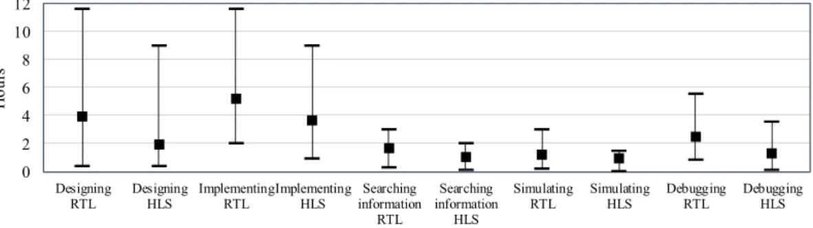
Fig. 8. Maximum, minimum, and average time usage for different categories with RTL and HLS. TABLE VII

AREA ANDPERFORMANCEFIGURES OFRTLANDHLS DESIGNS

TABLE VIII HLSANDRTL PRODUCTIVITY

TableVIIItabulates productivity values for HLS and RTL approaches. The productivity of all participants was clearly better with the HLS tool, and the average productivity of HLS was up to 6.0 times that of RTL. Hence, it is even higher than that found in the survey results. We can speculate how the

productivity would have changed if the persons had imple-mented stage pipelining in their RTL implementations. It is still unlikely that the productivity levels had shifted to support RTL over HLS, as the time usage would have increased along with the throughput.

Fig.8shows the time usage of the participants in five cat-egories. On average, the persons used less time within all categories when working with HLS. The grand total for max-imum, average, and minimum time usages with the RTL flow was 37.7, 15.1 and 3.7 h, respectively, whereas the same values for the HLS flow were 25.0, 10.1, and 1.6 h.

As a conclusion, all participants had better productivity with HLS than with RTL. Although the group size was small, and the hardware background of the persons was very similar, this study shows that it is easier to adopt HLS than RTL and receive better results faster for people who have most of their experience in software design. This result underlines the fact that HLS is a useful tool for software engineers who want to implement, for example, hardware accelerators.

It should be noted that our result differs from the typical surveyed study, where the QoR of RTL was better than that of HLS. The likely explanation for this is that in the sur-veyed works, the designers had significantly more previous hardware expertise than our test persons. On the other hand, our case study is in line with the surveyed literature concerning productivity, which favors HLS.

D. Feedback From the Test Persons

After completing the test assignments, the participants were asked about the pros and cons of HLS and RTL design flows, out of which they finally had to select their favorite. The answers were split evenly (3-3) between HLS and RTL flows. The persons favoring RTL over HLS hoped for more open source support for HLS tools, as the flow is highly tool depen-dent. This would allow more hobbyists to use HLS tools. Some test persons also wished for more control in the HLS tool over the resulting RTL in terms of cycle accuracy. For them, RTL was easier to fine tune and it gave them a better understanding of the problem at hand.

The persons favoring HLS over RTL liked the ease of HLS, where unnecessary details such as automatic I/O handshak-ing and pipelinhandshak-ing support can be left as the responsibility of the HLS tool. This let the participants to focus on defining the behavioral description. They also felt that RTL was more

Authorized licensed use limited to: Universita della Svizzera Italiana. Downloaded on August 23,2020 at 08:47:02 UTC from IEEE Xplore. Restrictions apply.

Figure 2.2. Comparison of HLS and RTL design flow productivities across different metrics. The boxplots show the maximum, minmum and average time for the different metrics evaluated. The figure has been published in [61].

reconfigurability of FPGAs well fits with the benefits introduced by HLS tools. In particular, the possibility to rapidly generate different IPs implementing a large variety of functionalities, and the efficient estimate of their performance and costs, make the combination of FPGA and HLS an extremely appealing solution for the design and deployment of complex systems on FPGA architecture [33].

In a recent work, Lahti et al. [61] have analysed different metrics comparing the HLS design flow with respect to the traditional RTL one. They have compared in particular the quality of result and productivity differences between the two. Their findings showcased that while the quality of results of the RTL flow is still better than state-of-the-art HLS tools, the average development time with HLS tools is much faster. The paper shows that a designer can achieve four times more productivity with HLS [61] with respect to the RTL flow. Figure 2.2, from [61] exhibits these differences. The chart shows the time required to implement different designs with the HLS and the RTL design flow. For all the different metrics considered in the study, the HLS flow resulted in higher productivity.

2.2.1 Evolution of HLS

The origin of HLS can be traced to the early 1970s. At that time, Carnegie Mel-lon researchers built a revolutionary tool (CMU-DA [30][88]) which, using the Instruction Set Processor Specification (ISPS) language[3], allowed the descrip-tion of a design at a behavioural level. By generating an intermediate represent-ation, common code-transformation techniques were applied, and the concepts of datapath allocation, module selection, and controller generation step of the modern synthesis tools were introduced for the first time. That work, despite little consideration from the industry[72], raised considerable research interest

(22)

[18].

The next decade, 1980-1990, has seen the proliferation of a number of dif-ferent research HLS tools (e.g., ADAM [44], HAL [90], MIMOLA [74], and Her-cules[27]), and few industrial ones (Cathedral [26], Yorktown Silicon Compiler [11] and BSSC [139]). These works, similarly to modern tools, decompose the synthesis process in different steps: code transformation, module selection, op-eration scheduling, datapath allocation, and controller genop-eration.

Code transformation is used to transform the original code into a semantic-ally equivalent version of it, able to better expose the program characteristics and allowing basic optimisations. The module selection phase selects, from a library of different components, the particular functional unit used to implement each operation in the code–e.g., it selects the most appropriate hardware multiplier to implement a multiplication among floats given a certain clock constraint. Op-eration scheduling assigns each opOp-eration into a specific cycle or control state. Then, datapath allocation defines the type and number of hardware resources needed to satisfy the design constraints, and, lastly, controller generation applies all the design decisions to generate an RTL model to be synthesised. All these steps were the cornerstone for the next generations of HLS tool.

A common characteristic of these tools was the adoption of custom languages to define the design specifications. Some of them used extensions of existing languages–i.e., Hercules[27] used HardwareC [60] based on the existing C lan-guage –while many others opted for custom lanlan-guages oriented to domain-specific applications. Despite these tools being the ancestor of the modern generations, only a few of them were widely adopted and obtained large consensus. Among them, the Cathedral project[26] had a long evolution and culminated in its com-mercialisation and the OptimoDE tool from ARM[17]. However, the poor quality of the results, the domain specialisation of most of the tools, the lack of a compre-hensive design language and the creation of many custom ones, combined with the adoption of RTL synthesis tools, spread the idea that behavioural synthesis could not fill the productivity gap[72].

In the next decade, 1990-2000, thanks to the improvement in RTL synthesis tools and the wide adoption of RTL-based designs, the major Electronic Design Automation (EDA) companies have invested in commercial HLS tools. Propriet-ary tools from Synopsys with Behavioural Compiler [59], Cadence with Visual Architect[49] and Mentor Graphics with Monet [34] entered the market. While these tools were able to raise the interest of industries, they could not replace the RTL design flow. In particular, the necessity of using behavioural description languages as input of the HLS tool, and the steep learning curve of those, lim-ited their diffusion. Moreover, the HLS design flow was still missing important

(23)

aspects. Existing tools failed to recognise the difference between data-flow and control flow, often focusing on only one of the two aspects resulting in poor qual-ity of results. Lastly, EDA were not able to correctly foresee potential user of HLS. These tools were thought for current RTL designers, who were skeptical about the newcoming design flow and relied on the quality of results of the traditional RTL-design flow[23]. This aspect made clear that it was necessary to raise the abstraction level of design languages, and to enlarge the pool of users to increase the diffusion of HLS tools.

The rise in abstraction level is the characterising aspect of the current gener-ation of HLS tools. The 21st century has mainly seen the evolution of existing behavioural CAD tools[13][119][24][117]. Despite different opinions [32][99], EDA companies and researchers realised the necessity to adopt a high-level input language, more accessible to algorithm and designers than HDLs. The choice fell on C/C++ and C-like languages–e.g., SystemC. This had a huge impact on the diffusion of HLS tools. It expanded the pool of users for HLS tools and allowed researchers to leverage the most recent compiler technologies and optimisation. This last aspect consequently resulted in an improvement in the quality of result of the HLS tools, making them more reliable and appealing to RTL-designers.

However, despite the large diffusion of C and C++ as dominating input lan-guages, these are used with limitations. Current HLS tools cannot exploit all the features of such languages such as pointers, dynamic memory management, recursion and polymorphism, which can hardly be mapped to a hardware imple-mentation. Moreover, C/C++ lacks some aspects such as definition of variable bit-width, timing, synchronisation, characterising the hardware design. To cope with this, many language extensions and libraries have been proposed[60][42] [120] and restriction to the C input programs have been introduced. Among these strategies, the use of pragmas, directives, and the adoption of a subset of ANSI C/C++ had large diffusion. By using pragmas and directives the HLS pro-cess can be guided, and standard compiler techonology can be adopted. This modularity allows to seamlessly move from software to hardware design in the direction of the hardware/software codesign goal.

Another important factor that favoured the diffusion of HLS tools was the growth of the FPGA market and the diffusion of this technology[124]. FPGAs, differently from ASICs, require different implementation programming models and have different design criteria. The limited resources available on a reconfig-urable chip force designers to explore different architectural choices able to fit area and performance constraints. The possibility to easily explore these costs and performance tradeoffs with the use of pragmas to govern the HLS process made HLS tool an appealing solution for designers targeting FPGA technology.

(24)

Many HLS tools flourished in the 2000 decade belong to this category like SPARK [116], ROCCC [98], Trident [125], Handel-C [46] among many.

A more recent evolution of HLS tools has seen the diffusion of research-oriented projects as Bambu [92], LegUp [12] and AutoPilot [144], with few of them, Autopilot and LegUP, being acquired by EDA companies or commercial-ised respectively. Among commercial tools, VivadoHLS [126], CatapultC [13], Bluespec[7] and CtoS [117] had large diffusion. Lastly, the 2015 acquisition of Altera from Intel lead to the creation of the recent Intel HLS Compiler[53], and the recent integration of FPGAs on the Amazon Web Services architecture has seen the adoption of the Xilinx design suite SDAccel[109].

2.2.2 The HLS Process

In the previous sections, we have mentioned the benefit of the HLS design flow and the evolution that HLS tools had from the 70s until today. Herein, I will describe the HLS process’s details and the steps performed by synthesis tools to automatically generate an RTL implementation starting from a C/C++ design. An experienced reader, who is already aware of the HLS process details, may want to skip this section and move to the next ones.

The HLS process provides many benefits to designers, it allows, starting from a high-level description of an application, the rapid generation of optimized RTL specifications. By focusing only on the behavioural aspect of the functional-ity to implement in hardware, designers can reason on what to implement in-stead of how to achieve that. Moreover, HLS enables rapid exploration of micro-architectural variations through the use of optimisation directives. Thus, mul-tiple variants of the same circuit functionality can be seamlessly implemented satisfying different cost and performance requirements. Besides, the adoption of HLS simplifies the verification process and the portability of the generated IPs.

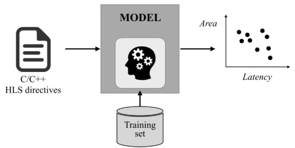
To generate an RTL implementation, the HLS process requires a high-level specification of the functionality to implement in hardware, an RTL component library, and a set of design constraints–e.g., target architecture, clock period. Given these elements, the HLS process relies on five different steps: compilation, resource allocation, operation scheduling, binding, and control logic generation. All these steps break down the original behavioural representation, extract the operations and variable describing the functionality, and use this information to generate the final RTL implementation.

In the following, the different steps are detailed, and a few practical examples are provided. Figure 2.3 shows an overview of the HLS-design flow, including the required input, the process steps, and the generated output.

(25)

11 2.2 High-Level Synthesis Revolution Compiler pass High-level specifications Technology

library constraintsDesign CDFG Resources allocation Scheduling Binding Control logic generation RTL specifications

Figure 2.3. Overview of the HLS process.

Compiler pass

The input specifications are processed by a compiler pass which generates and ab-stract representation of the functionality. The compiler extracts the information needed to identify the resources and the operations to be implemented in hard-ware. The compiler pass defines "what" will be implemented. In this phase, the compiler may introduce code optimisations, either to simplify the code structure– e.g., dead code elimination, constant propagation, and loop transformation may be applied–or to transform the original code into a functional equivalent version that can be mapped to a more efficient design pattern.

Standard abstract representation of the code are Control Data Flow Graphs (CDFGs)[41][84]. CDFGs encompass both the data and control dependency in-formation between operations. These are built extending the Data Flow Graph (DFG) with control flow dependencies in order to represent loop structures and unbounded iterations. The CDFG nodes and the edges identify the set of opera-tions and variables needed to generate the RTL implementation. These elements are the input of the allocation, scheduling, and binding steps.

Resources Allocation

Once the variables and the operations have been extracted by the compiler, the resources required to map them to hardware are defined. Allocation defines "who" will perform the identified operations. This step, named resource alloca-tion or simply allocaalloca-tion, defines the type and number of funcalloca-tional units, stor-age components, busses, and other connectivity elements required to generate

(26)

the hardware implementation. The available resources are selected from a lib-rary of RTL components, usually dependent on target technology and proprietary tools. This library includes all the information required by the synthesis task to estimate area, power, and latency needed in the scheduling and binding phases.

Scheduling

The scheduling phase maps all the identified operations to a specific clock cycle. This step defines the order in which each operation will occur. Scheduling de-termines "when" an operation will happen. Design constraints and the techno-logy library have a significant impact on the resulting schedule. E.g., by relaxing the clock period constraint more operation may be scheduled into the same clock cycle, according to technology characteristics. Similarly, using a faster techno-logy, more operations may occur during the same cycle.

In addition to technology and design constraints, the code structure also has an impact on scheduling. For example, the concatenation of operation interme-diate results may lead to a more efficient scheduling of the operations.

Figure 2.4 shows examples of scheduling given the resource allocations for two different types of technologies and different design constraints–i.e., clock constraint.

Binding

Binding determines which allocated resource will be used for each operation. Binding defines "where" operations are mapped to the allocated resources. Oper-ators are mapped to functional units, and variables are mapped to storage units. In this phase, decisions about the sharing of the allocated resources are made. According to the performance or power/area requirement, the binding phase will decide to allocate more units or share the functional and storage units already allocated among the different operations and variables. These choices may affect the resources required for the connection of the allocated resources. Therefore, some of the choices affecting the connectivity elements performed during the allocation step may be revised at this stage.

Figure 2.4 scheduling d) shows an example of binding with resource sharing. Resources are re-used during the scheduling in order to minimise the area and reduce the number of functional units.

(27)

13 2.2 High-Level Synthesis Revolution int foo(…){ … tmp1 = a + b; tmp2 = tmp1 * c; tmp3 = d + e; res = tmp2 - tmp3; } Allocated resources: + + a b c d e tmp1 tmp2 tmp3 res -+ + * * -+ + * -Scheduling: + * + -+ + * -Technology 1 Technology 2 Technology 1 3 cycles Technology 2 4 cycles + + -Technology 1 2 cycles (slower clock) Scheduling with binding sharing resources:

+ + -Technology 1 4 cycles (less resources) * * a) b) c) d)

Figure 2.4. Example of resource allocation, scheduling, and binding for the code in the example. Four different scheduling are shown: a) scheduling adopting functional units of technology 1, b) scheduling adopting functional units of technology 2, c) scheduling adopting functional units of technology with a slower clock constraint from the one originally specified by the designer, d) scheduling adopting functional units with binding sharing resource. In the last scheduling example, only one adder is allocated, and the same functional unit is used to compute both tmp1 and tmp3 at different clock cycles.

Control Logic Generation

The last step of the HLS process generates the final RTL architecture. The con-trol logic extracted by the compiler pass is used to define the datapath for the functionalities implemented in the previous steps. The datapath includes all the storage elements, functional units, and connection elements defined in the alloc-ation and binding stages according to the defined scheduling. Input, output, and control ports of the design interface are connected to the RTL logic, and a finite state machine implementing the controller unit manages the correct execution of the functionality.

(28)

Putting all together

All the above-mentioned steps together generate the resulting RTL. While per-forming independent tasks, the different phases are affected by the decisions made by each other. In particular, allocation, scheduling, and binding choices are interdependent. For this reason, these three stages are the core of the exist-ing HLS tools and are the ones characterisexist-ing their quality of results.

The efficiency of these different stages may also impact the target techno-logy of HLS tools. For example, HLS tools targeting FPGAs may be interested in resource-constrained approaches. In this case, the allocation process and a binding sharing the resources will be predominantly imposing more stringent constraints on the scheduling. In other cases, e.g., for time-constrained applica-tions where ASICs are the target technology, more aggressive scheduling will be adopted.

Moreover, these stages are performed in order to satisfy a target objective function, such as the minimisation of area/power or latency. Some HLS tools allow designers to chose the target objective–i.e., Mentor Catapult HLS [13]– while others are optimised for one of the two–i.e., VivadoHLS [126] minimises the latency. However, even for HLS tools where the objective function is prede-termined, time and resource requirements can be satisfied by relaxing the design constraints.

While HLS can automatically generate efficient RTL implementation of the given functionality, designers do not directly control its process. To cope with this aspect, HLS tools allow designers to guide the synthesis through HLS dir-ectives. These directives, often in the form of compiler’s pragmas, directly affect the compiler pass, allocation, scheduling, and binding steps. In the following, a description of the most common optimisations and some practical examples are provided.

2.2.3 HLS Optimisations

HLS tools, by specifying HLS directives, can influence the synthesis process. The directives directly impact the resulting performance and costs, enabling designers to rapidly explore different architectural variations. The number and type of possible optimisations depend on the HLS tool. However, across the different tools available, some macro-categories of optimisations are common. Herein, these will be described, and a few examples of their effect will be discussed. In particular, I will discuss the pragmas available for the VivadoHLS tool[126]. While directives names may differ according to the commercial tool adopted, the

(29)

effect they have on the synthesis process is similar.

Spatial Parallelism

One of the most common optimisation is spatial parallelism. Spatial parallelism allows to reduce latency and increase the throughput of an IC. Multiple func-tional units can be instantiated to concurrently execute the program operations. HLS tools automatically perform instruction-level parallelism during the schedul-ing and bindschedul-ing phase. However, designers can force the amount of parallelism by explicitly specifying regions of the code to be parallelised. For example, a designer can target a loop with an unroll directive. The directive forces the com-piler to unfold the loop body up to a certain factor, or even entirely, imposing to the HLS tool to instantiate the hardware resources required to execute the loop body operations concurrently. Ideally, a loop without loop carried depend-encies can be parallelised entirely if enough resources are available. Therefore, the execution time of the entire loop is reduced to the execution time of a single iteration. Usually, spatial parallelism dramatically reduces latency but requires a significant amount of extra resources.

Figure 2.5 shows an example of a loop unrolling directive applied to a loop. The optimisation, specified in the form of pragma in the original code, unrolls the loop by a factor of 2. Therefore, the functional units in the loop’s body are doubled, and the total number of iterations required to execute the loop is halved.

Pipelining

Another common optimisation among HLS tools is pipelining. Pipelining can be applied to functions or loops, and it reduces the initiation interval for functions or loops allowing concurrent execution of their operations. In fact, the execu-tion of the next loop or funcexecu-tion input can start before the compleexecu-tion of the predecessor’s operations. Pipelining requires that data dependency must be re-spected before moving to the next iteration. Pipelining enables functions and loops to process a new input or loop iteration every N cycles, where N is the Initiation Interval (II). The II specifies the number of clock cycles between suc-cessive input processing or loop iterations. The ideal II of 1 specifies that a new input or loop iteration should be processed every cycle. However, the minimum II achievable can be limited by resource constraints or dependencies–i.e., loop carried dependencies. This optimisation, similarly to spatial parallelism, implies the allocation of extra resources required to perform the parallel execution of multiple input/iterations, but it may greatly improve execution time. Compiler

(30)

int foo(…){ …

loop:for(i=0;i<10;i++){

#pragma HLS unroll factor=1

tmp1[i] = a[i] + b[i];

res[i] = tmp1[i] * tmp1[i];

} }

int foo(…){ …

#pragma HLS unroll factor=2

tmp1[i] = a[i] + b[i];

res[i] = tmp1[i] * tmp1[i];

} } Allocated resources: + * + * Scheduling: + * … i = 0 i = 1 20 cycles to perform loop body computations Allocated resources: + * + * Scheduling: + * … i = 0 i = 2 + * + * + * … 10 cycles to perform loop body computations i = 1 i = 3

Figure 2.5. Examples of loop unrolling directives applied on a loop. (Top) Allocated resources required by the loop body computation and an example of scheduling for them when no unrolling is applied. (Bottom) Allocated resources and schedule when a loop unrolling factor of 2 is applied. The number of iterations is halved, and the amount of resources is doubled. For simplicity, the computation required to increment the loop iterator variable and check the loop condition are omitted in both examples.

passes can be combined to greatly improve the effectiveness of this optimisation [131][151].

Figure 2.6 shows an example of the pipeline directive applied to a loop. The optimisation, specified in the form of pragma in the original code, defines an initiation interval of 1. The loop body instructions are pipelined allowing the execution of each operation at a new cycle.

Memory Allocation

While implementing a design in hardware, different choices regarding the mem-ory allocation strategy are possible. Private Local Memories (PLM) can be coupled to accelerators to allow direct access to the data needed during computation. In FPGAs, this can be easily achieved by forcing the allocation of multiple memory banks in the form of distributed block RAMs (BRAMs). Using PLM, accelerators can perform multiple memory operations in one cycle according to data distri-bution over the allocated memories. However, allocation of specific resources is

(31)

int foo(…){ …

#pragma HLS pipeline II=1

tmp = A[i]; // RD tmp = tmp * tmp; // CMP res[i] = tmp1; // WR } } int foo(…){ … loop:for(i=0;i<10;i++){ tmp = A[i]; // RD tmp = tmp * tmp; // CMP res[i] = tmp; // WR } } Allocated resources: Scheduling: RD CMP WR Allocated resources: Scheduling: i = 0 i = 2 i = 1 … RD CMP WR RD CMP WR i = 0 i = 1 i = 2 RD CMP WR RD CMP WR RD CMP WR … RD CMP WR RD CMP WR

Figure 2.6. Examples of pipelining applied on a loop. (Top) Resource and scheduling required by the loop body without the pipelining directive. Nine clock cycles are required to perform three iterations of the loop. (Bottom) Allocated resources and scheduling with loop pipelining enabled with an initi-ation interval of one. Five clock cycles are required to perform three iteriniti-ations of the loop.

required. These resources depend on the available technology library and the target platform. Therefore, available resources may be limited to a certain type and size.

Designers can force the HLS tools to instantiate particular memory elements and allocate design variables to instantiated memories. However, forcing the use of a specific memory element and type can result in suboptimal use of resources if the design variables’ size is not aligned to the memory sizes.

Moreover, HLS tools permit to change the physical implementation of the memories by specifying memory partitioning directives. Memories usually have only a limited number of read and write ports, which can limit the throughput of a load/store intensive algorithm. According to the original code’s memory ac-cess pattern, the bandwidth of an allocated memory element can be increased by partitioning the memories associated with the arrays in the original code. The original array elements can be distributed over multiple smaller memories, effect-ively increasing the number of load/store ports. While potentially improving the throughput of the design, this optimisation requires more memory instances or

(32)

18 2.2 High-Level Synthesis Revolution 0 1 2 3 4 5 0 1 2 3 4 5 0 1 2 3 4 5 0 1 2 3 4 5 A A A

Mem 1 Mem 2 Mem 3 Mem 4 Mem 5 Mem 6

0 1 2 3 4 5 Memory 1 Memory 2 Block 0 2 4 1 3 5 Memory 1 Memory 2 Cyclic Complete

Figure 2.7. Examples of array partitioning directives applied to an array vari-able. (Top) Block array partitioning with partitioning factor of 2. (Middle) Cyclic array partitioning with partitioning factor of 2. (Bottom) Complete partitioning.

registers and increases the connectivity element among memory and functional units.

Figure 2.7 shows an example of the array partitioning directive applied to three arrays. The figure shows three different types of partitioning strategies– block, cyclic, and complete–and partitioning factors. A block strategy partitions the original memory into equally sized blocks of consecutive elements. A cyc-lic partition splits the original memory into same size memories interleaving the elements of the associated array. In this case, consecutive array elements are dis-tributed on different memory elements up to a certain partitioning factor. Com-plete partitioning instead is the most resource expensive approach. It comCom-pletely decomposes the memory into individuals elements.

Predicated Execution

Software transformations can be applied to allow a parallel schedule of disjoint execution paths. This transformation of the code, often named if-conversion, re-quires the introduction of predicates, or guards, to discriminate at the end of the parallel execution among the concurrent paths’ results. The benefits of pre-dicated execution are a higher parallelisation of the code and the elimination of

(33)

control dependency in the execution of intensive code structures. This optimisa-tion is extremely effective in the case of balanced branches, while in the case of unbalanced, the execution time could even be slowed down.

Hierarchical-Module Optimisations

By removing or introducing hierarchy among the generated modules, the amount of control logic generated by the synthesis may be affected. For example, en-abling function inlining avoids execution and generation of the logic required to manage function invocations. The inlining HLS directive flattens the hier-archy among target function and remaining RTL code. Therefore, the function no longer appears as a separate hierarchy level in the RTL, and a better resource sharing can be achieved. On the other hand, an inlined function cannot be shared, and the reuse of its RTL module is not possible. This optimisation may reduce the overall latency, but more area is usually required to implement the RTL. Similar results can also be obtained for loops by merging the body of the loops.

Bit-width Optimisation

This optimisation specifies the exact amount of bits required by datapath oper-ators and variables. Differently from general-purpose processors, which are de-signed with a fixed size datapath, HLS tools can generate specialised hardware with custom size operators and registers. This optimisation affects all aspects of the resulting implementations: area, latency, power, and quality of the gener-ated output. It enables to minimise the area of a design while satisfying certain task-related quality of result goals. For example, the implementation of com-plex machine learning models (i.e., Convolutional Neural Networks) on ASICs and FPGAs relies on the identification of the optimal bit-width for the neural network layers [129]. In this case, reducing the bit-width allows to dramatic-ally diminish the model’s size and the memory required to store it. This aspect is extremely beneficial since it permits to deploy complex models on resource-constrained platforms. The main drawback of this approach is related to the effect that bit-width reduction has on the quality of the implemented acceler-ator’s results. In fact, for classification tasks reducing the bit-width significantly affects classification performance. While targeting these applications, designers then have to evaluate the results of the generated hardware to verify that a target classification goal is satisfied.

(34)

20 2.3 New Challenges

Resource Library

The allocation step of the HLS process identifies, from a library of RTL compon-ents, the resources needed to implement the desired functionality in hardware. Existing libraries are rich and offer several different implementations of the same operation. However, it is hard for designers to foresee the choices made by the HLS tools and estimate the result of the synthesis process. The different com-ponents available in these libraries are often vendor-specific or related to the target technology and a characterisation of the library components is not always available.

Through the use of HLS directives, designers can force or prevent the use of specific resources affecting the allocation step, and, consequently, the HLS process results. Enforcing the use of particular resources allows designers to control more tightly the HLS process. Moreover, while designers may have a higher degree of control on the HLS process, the implemented design is generated minimising a target objective during the synthesis. Forcing the use of certain resources may lead to suboptimal choices unless specific resource constraints are required

2.3 New Challenges

The HLS revolution has shaken the belief of hardware designers about the capab-ility of HLS tools. The dramatic gain in the design productivity introduced by the HLS design flow and the quality of results achievable with existing commercial and research tools have consolidated HLS as a viable option for fast prototyping and short-time-to-market[61][18].

However, many of the advantages of HLS are hardly quantifiable with re-spect to traditional design flows. For example, HLS allowed designers to explore a space of possible optimisations for their design that, before HLS, was hardly treatable. The quality of resulting implementations was dependent on the de-signer experience, while, nowadays, structured and sound search strategies can be applied to identify effective optimisations.

On the other hand, the possibility of rapidly exploring equivalent versions of the same design has opened a new challenge. Navigating the space of all the possible implementations controlled through HLS directives is a non-trivial task. This problem, namely the Design Space Exploration (DSE) problem, requires the identification of the most effective combination of optimisations for a given design and engineer target requirements. In this dissertation, we focus on this

(35)

21 2.3 New Challenges

challenge.

However, DSE is not the only challenge introduced by HLS. Another one is the identification of which portion of the software to accelerate in hardware. Not all software benefits in the same way from hardware acceleration, and complex heterogeneous systems must be properly designed to benefit from heterogeneity and hardware specialisation. To this end, various works have been proposed [143][142], and research in this area is extremely active.

Other challenges involve the improvement of in-system design validation and debugging, better support for domain-specific synthesis, and the possibility of raising the level of abstraction moving to higher level languages (i.e. Python) among others.

(36)

(37)

Chapter 3 The Design Space Exploration Problem

In this chapter of the dissertation the terminology and a formal definition of the HLS-driven Design Space Exploration (DSE) problem are presented. In addition, a metric, used to evaluate the quality of the DSE and to perform a comparison with respect to the state of the art alternatives is introduced.

Section 3.1 will describe the terminology adopted in this document to dis-criminate among the different elements of the HLS design flows. In Section 3.2 a formal definition of the DSE problem and the elements characterising it will be presented. Finally, 3.3 will introduce the metric used to evaluate the quality of the DSE methodologies.

3.1 Terminology

An HLS design (or design) is a functionality to be realized in hardware. For ex-ample, a Fast Fourier Transform function and a 2D convolution function from an image processing application are examples of designs that can be separately synthesized with HLS. A specification is a high-level description of the design in a programming language such as SystemC or C/C++. The specification, which can be given with an untimed or a loosely-timed model, is the input to the HLS tool. An implementation of the design is the output of a run of the HLS tool. This output is typically expressed as an automatically generated RTL code written in Verilog or VHDL. Each implementation is characterized by the values of a per-formance metric and a cost metric (e.g., latency or throughput as perper-formance metric and, area or energy as costs).

A synthesis configuration (or, simply, configuration) defines the transform-ations that a design undergoes through HLS. A designer controls these trans-formations with constraint and optimization directives, such as loop unrolling or

(38)

24 3.1 Terminology

Listing 3.1. Example of specification in C for a toy example design.

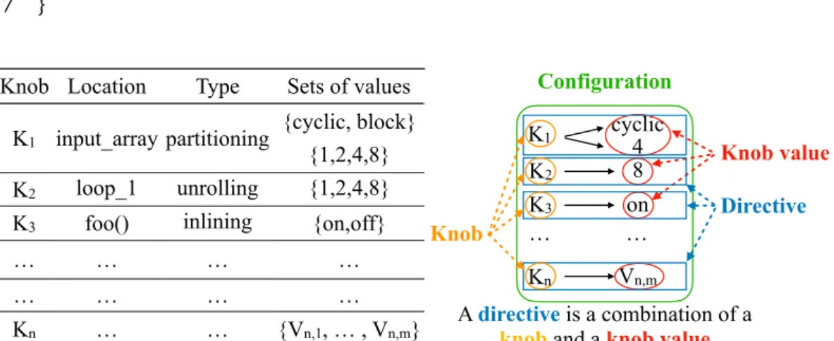
1 void bar ( i n t i n p u t _ a r r a y[32] , i n t output_array [32]) { 2 i n t i ; 3 loop_1 : f o r ( i=0; i <32; i ++){ 4 o u t p u t _ a r r a y[ i ] = input_array [ i ]*input_array [ i ] ; 5 } 6 f o o ( o u t p u t _ a r r a y ) ; 7 } Vn,m Knob Location Type Sets of values

K1 input_array partitioning

{cyclic, block} {1,2,4,8} K2 loop_1 unrolling {1,2,4,8} K3 foo() inlining {on,off}

… … … … … … … … Kn … … {Vn,1, … , Vn,m} K1 cyclic ₄ 8 Knob value Directive Configuration Knob A directive is a combination of a

knob and a knob value

on … K2 K3 Kn …

Figure 3.1. Example of terminology associated to the example in Snippet 3.1.

pipelining, array manipulation, and other control and datapath optimizations. A directive is associated with a location in the code specification. A location could be either a label in the code or a language construct; for example, a loop or an array declaration. A designer can further customize some directives by specifying the values for the directive parameters–for example, the designer can customize the amount of parallelism in the implementation by unrolling a loop a certain number of times or by setting a certain initiation interval for the pipeline imple-menting the loop.

Each location of a given specification, with an associated directive, encodes a knob (a type of directive, the location, and selected parameter values) that the designer considers for the DSE task. For each directive a designer can manually define an admissible set of directive values, and, for directives with multiple parameters (i.e., partitioning allows to specify both the factor and the type), a set of values for each parameter is specified.

Example: Snippet 3.1 and Figure 3.1 show an example of specification for a target design–functionbarin the snippet–and the associated notion of directive, knob, knob type, location and set of values associated to a directive for possible

(39)

25 3.2 Problem Formulation

targets in the design.

For a design D, letXDdenote the set of all possible synthesis configurations. In general,XDis a very large set, possibly of infinite size. In practice, designers explore a portion of the design space of D by trying a subset XD ⊂ XD, whose elements they choose carefully based on their experience running HLS.

The set of all the possible configurations explored by a designer is the Con-figuration Space(XD). This is defined as the cartesian product among the sets of directive values for each knob:

X_D= K1× K2× · · · × KN (3.1) where N is the number of considered knobs, and Ki is the set of values related to each i knob, i.e. the set of values that the directive associated to knob i can as-sume. For a directive with multiple parameters–e.g., array partitioning requires to define both the partitioning factor and the type–, Ki is the Cartesian product among each set of values. The size of the configuration space is then given by its cardinality (|XD|).

Lastly, the design space (YD) is the set of implementations resulting from the synthesis of the configuration is XD.

3.2 Problem Formulation

The DSE of an HLS design is a multi-objective optimisation problem, with costs and merit as objective functions. In literature different objective functions have been considered for the DSE problem. The survey from Bulnes et al. [97] iden-tifies the following as the most common objectives considered in the state of the art:

• Latency. This is the most common unit of measure for the performance. It is usually defined as the number of clock cycles required by a hardware im-plementation to complete its functionality. Alternatively, the total latency is multiplied with the target clock of the system. In this case the objective is referred as effective latency.

• Throughput. Ratio among the effective latency and the input size. It meas-ures how efficiently the input is processed with respect to its size.

• Area. This is the most common unit of measure for the costs. It can be either the space occupied to implement the IC in hardware, expressed in

(40)

µm2_{, or the number of components allocated in the target device, i.e.}

func-tional units (FU) and registers. While the first is commonly used for ASIC, the second approach is well suited for reconfigurable resources as in the case of FPGA. I this cases common units of measure are the number of Flip-Flops (FF), Look-Up Tables (LUT), Digital Signal Processor (DSP), and Block RAM (BRAM).

• Resource utilization. With FPGA, due to the limited number of resources available on a target device, the costs is expressed as percentage of re-sources required by an implementation. With such formulation, multiple different resources can be aggregated together in a single objective func-tion.

• Power. Total power consumption of the IC. This is usually the combination of dynamic and static power consumptions.

• Wire length or Data path. Measure of costs of the interconnection and of the connectivity components.

• Digital noise. Measure of error due to the combination of computational errors and noise propagation introduced by bit-width reduction and quant-isation effects.

• Reliability. Measure of probability that an error will occur due to soft errors. This usually depends form the type of FU used in the design.

• Temperature. Measure of maximum temperature and temperature vari-ation occurring during the execution of the design functionality. Usually minimised to reduce electronic failures.

• Robustness. Protection that a IP offers against attacks, i.e. reverse engin-eering attacks.

In the context of my works I have considered as measure of cost the area (a), expressed either as the number of FF, LUT, DSP, and BRAM, or as aggregated values of those in form of a linear combination of their utilisation for a given technology: a= FF FF_{avail a bl e} + LUT LUT_{avail a bl e} + DSP DSP_{avail a bl e} + BRAM BRAM_{avail a bl e} (3.2)

(41)

Equation 3.2 allows to evaluate the overall utilisation of the resources required by an implementation (FF, LUT, DSP, and BRAM) with respect to the ones available on a specific FPGA (FFavail a bl e, LUTavail a bl e, DSPavail a bl e, and BRAMavail a bl e).

As a measure of merits I have considered either latency and effective latency (l). Where the effective latency is measured as the product among the clock cycles and the clock period.

l= #Clock_c ycles × Clock_period (3.3) The resulting area a and latency l obtained for a given configuration through the HLS process define the implementation cost and merit.

Goal of the DSE problem is to identify the Pareto-optimal implementations of a given design while minimising the number of synthesis required to implement them. Given D and XD, the design space exploration task returns a subset of XD that consists of all Pareto configurations, i.e.

P(D, X_D) = {x|x ∈ X_D and x is Pareto} (3.4) A Pareto configuration (p) of a design is a configuration that leads to an imple-mentation that is Pareto-optimal in the bi-objective optimization space defined by the performance and cost metrics.

A (first-rank) Pareto frontier (P(D, X_D), or, simply, P) is the set of points: p_{∈ P ⇔ > q ∈ X}_D, q6= p | A(q) ≤ A(p) ∧ L(q) ≤ L(p).

Where A(·) and L(·) are the area and latency values associated to a configuration. In other words, iff p ∈ P, then no other solutions exist in the design space having simultaneously less area and less latency than p.

A (first-rank) Pareto frontier is the set of Pareto-optimal points. Finally, an i-th rank Pareto frontier(for i> 1) is defined as the Pareto frontier obtained after removing the lower rank frontiers from the design space.

Figure 3.2 shows examples of different ranked Pareto frontiers.

DSE strategies aim at finding an approximate Pareto frontierbP(D, X_D) of the best performing implementations, as close as possible to the one deriving from exhaustive search P(D, X_D), while minimizing the number of synthesis runs.

(42)

28 3.3 Metrics Area Latency Area Latency Area Latency Figure 3.2. Example of three different rank Pareto frontier. (Left) 1st-rank Pareto frontier. (Center) 2nd-rank Pareto frontier. (Right) last rank Pareto frontier.

3.3 Metrics

Quality evaluation of DSE is a challenging aspect. In literature a variety of met-rics have been adopted to measure the results of the DSE process. Different works [91] [22] [21] measure the improvement obtained by an optimised im-plementation with respect to a standard one–e.g., the one generated by the HLS tool without applying directives. For a given implementation the performance and area improvement and/or reduction are measured and compared with the ones obtained with different methodologies. While this approach offers an im-mediate view on the effectiveness of a given implementation it doesn’t highlight the ability of a methodology to explore concurrently the design space objectives. To deal with this problem, Zitler et al. [149] suggested the use of the follow-ing metrics:

• Average Distance from Reference Set (ADRS). The ADRS metric expresses the distance between a reference curve P (the Pareto frontier from ground truth data), and an approximated curve bP. The ADRS for two objective functions is defined as:

ADRS(bP, P) = ₁ |P| X p∈P min b p∈bP(d(b p, p)) (3.5) b

P and P are the set of points defining the approximated Pareto frontier and the reference one, respectively. |P| defines the cardinality of the ref-erence set P and d(bp, p) is the distance among a reference point and an approximated one defined as:

(43)

29 3.3 Metrics d(bp, p) = max § 0,Abp− Ap A_p , L b p− Lp L_p ª (3.6) Given this formulation, low ADRS values are better, because they imply proximity between P and bP.

• Hypervolume or S-metric or Lebesgue measure. This metric is used to meas-ure the difference among hypervolumes (HV) between the approximated Pareto curvebP and the reference Pareto-set P. The HV of a set of solutions measures the size of the portion of the objective space that is dominated by those solutions collectively[134]. It requires the definition of a bounding point to calculate the volume of design space. Given a 2D design space, the HV measures the difference in area among the region of design space com-prised between the bounding point and the Pareto-front P with respect to the area of the bounding point and the approximated Pareto curvebP. A low difference among HVs implies a good approximation of the Pareto frontier. • Pareto Dominance. This metric measures the relation among the number Pareto-optimal design discoveredbP, and the one in the reference Pareto-set P. This relation is defined as:

Dominance= |bPT P|

|P| (3.7)

A high dominance score implies a good exploration result.

• Cardinality. This metric lists the Pareto solution discovered. High cardin-ality implies a larger variety of solution discovered. While this metric does not require a reference set to be calculated, it does not guarantee a good exploration quality.

Among the above mentioned metrics, with the exception of the cardinality metric, a ground-truth is required to compute the metric score. However, retriev-ing the reference Pareto-set P requires the exhaustive exploration of the design space and such process can be extremely time consuming if not infeasible. This aspect has often limited the use of such metrics as measure of the quality of results.

In my works, similarly to[64],[71],[86],[114],[138],[146], I have evaluated my methodologies by adopting the ADRS metric, measuring the distance among the Pareto-frontier retrieved by a given strategies with respect to a ground-truth. This approach, while requiring the exhaustive synthesis of the configuration space

(44)

30 3.3 Metrics 0 0.2 0.4 0.6 0.8 1 Latency 0 0.2 0.4 0.6 0.8 1 Area

DSE comparison: Exhausitve vs Heuristc

Figure 3.3. Example of an exhaustive exploration compared with an explora-tion heuristic. The x are the result of exhaustive exploration, while the dots (dark and light) are the design points explored by our heuristic (13% of the total). Dark dots represent the retrieved Pareto solution.

defined by the designer, allows a comparison with existing methodology which is both qualitatively with respect to the state of the art alternatives and with respect to the design space of the target design.

Figure 3.3, shows an example of DSE performed fordecodebenchmark from CHStone [47]. The synthesised configurations are marked with filled dots, non synthesised ones with crosses, and Pareto-optimal solutions of the design space with darker dots. The two objective functions considered in this DSE are the area, as a number of FF, and the latency, in number of clock cycles. An ADRS of 0.0128 was achieved with only 234 synthesis runs (over 1728 possible configuration).