An Extensive Investigation of Machine Learning Techniques for Sleep Apnea Screening

HAL Id: hal-02972546

https://hal.archives-ouvertes.fr/hal-02972546

Submitted on 12 Nov 2020

HAL is a multi-disciplinary open access

archive for the deposit and dissemination of

sci-entific research documents, whether they are

pub-lished or not. The documents may come from

teaching and research institutions in France or

abroad, or from public or private research centers.

L’archive ouverte pluridisciplinaire HAL, est

destinée au dépôt et à la diffusion de documents

scientifiques de niveau recherche, publiés ou non,

émanant des établissements d’enseignement et de

recherche français ou étrangers, des laboratoires

publics ou privés.

An Extensive Investigation of Machine Learning

Techniques for Sleep Apnea Screening

Jose Rodrigues, Jean-Louis Pepin, Lorraine Goeuriot, Sihem Amer-Yahia

To cite this version:

Jose Rodrigues, Jean-Louis Pepin, Lorraine Goeuriot, Sihem Amer-Yahia. An Extensive Investigation

of Machine Learning Techniques for Sleep Apnea Screening. CIKM ’20: The 29th ACM

Interna-tional Conference on Information and Knowledge Management, 2020, Virtual Event Ireland, France.

pp.2709-2716, �10.1145/3340531.3412686�. �hal-02972546�

An Extensive Investigation of Machine Learning Techniques for

Sleep Apnea Screening

Jose F. Rodrigues-Jr

Sao Carlos, SP, Brazil

Jean-Louis Pepin

Grenoble, France

Lorraine Goeuriot

Sihem Amer-Yahia

ABSTRACT

The identification of Obstructive Sleep Apnea (OSA) relies on labo-rious and expensive polysomnography (PSG) exams. However, it is known that other factors, easier to measure, can be good indicators of OSA and its severity. In this work, we extensively investigate the use of Machine Learning techniques in the task of determining which factors are more revealing with respect to OSA. We ran ex-tensive experiments over 1,042 patients from the Centre Hospitalier Universitaire of the city of Grenoble, France. The data included ordinary clinical information, and PSG results as a baseline. We em-ployed data preparation techniques including cleaning of outliers, imputation of missing values, and synthetic data generation. Fol-lowing, we performed an exhaustive attribute selection scheme to find the most representative features. We found that the prediction of OSA depends largely on variables related to age, body mass, and sleep habits more than the ones related to alcoholism, smoking, and depression. Next, we tested 60 regression/classification algorithms to predict the Apnea-Hypopnea Index (AHI), and the AHI-based severity of OSA. We achieved performances significantly superior to the state of the art both for AHI regression and classification. Our results can benefit the development of tools for the automatic screening of patients who should go through polysomnography and further treatments of OSA. Our methodology enables exper-imental reproducibility on similar OSA-detection problems, and more generally, on other problems with similar data models.

KEYWORDS

obstructive sleep apnea screening; machine learning; decision trees; naive Bayes

ACM Reference Format:

Jose F. Rodrigues-Jr, Jean-Louis Pepin, Lorraine Goeuriot, and Sihem Amer-Yahia. 2020. An Extensive Investigation of Machine Learning Techniques for Sleep Apnea Screening. In Proceedings of the 29th ACM International Conference on Information and Knowledge Management (CIKM ’20), October 19–23, 2020, Virtual Event, Ireland. ACM, New York, NY, USA, 8 pages. https://doi.org/10.1145/3340531.3412686

Permission to make digital or hard copies of all or part of this work for personal or classroom use is granted without fee provided that copies are not made or distributed for profit or commercial advantage and that copies bear this notice and the full citation on the first page. Copyrights for components of this work owned by others than ACM must be honored. Abstracting with credit is permitted. To copy otherwise, or republish, to post on servers or to redistribute to lists, requires prior specific permission and/or a fee. Request permissions from permissions@acm.org.

CIKM ’20, October 19–23, 2020, Virtual Event, Ireland © 2020 Association for Computing Machinery. ACM ISBN 978-1-4503-6859-9/20/10. . . $15.00 https://doi.org/10.1145/3340531.3412686

1

INTRODUCTION

Obstructive Sleep Apnea (OSA) is the predominant type of sleep breathing disorder; it is characterized by repeated episodes of com-plete or partial obstructions of the upper airway while sleeping, usually associated with a reduction of the blood oxygen saturation. OSA has the potential of reducing the quality of life and increasing the risks of cardio-vascular comorbidities [10]. Yet, a great part of the patients that suffer from OSA is not detected [13]. The detection of OSA is based on the results of a polysomnography exam, which records brain waves, blood oxygen level, heart rate and breath-ing, eye and leg movements during hours of monitored sleep. For OSA diagnosis, the Apnea-Hypopnea Index (AHI) measured by polysomnography breathing monitoring is the gold standard. How-ever, polysomnography is a laborious and expensive exam carried out on a limited basis, when OSA is already suspected in a patient. Rather than polysomnography, simpler tests in the form of di-rect observations, i.e. questionnaires, are used for screening OSA patients. However, according to AlGhanim et al. [2], even the best-validated test, the “STOP-BANG”, is limited when used for screen-ing based on only eight questions [16]. Another test, the Epworth Sleepiness Scale has minimal OSA-detection capabilities [5]. And the Berlim Questionaire heavily varies in terms of sensitivity and specificity, revealing its impreciseness in several clinical scenar-ios [6]. By inspecting such questionnaires, one can argue that the pieces of evidence that they collect are fail-proof as, for example, “Has anyone Observed you Stop Breathing or Choking/Gasping during your sleep?” But, still, they fail in a significant number of situations denoting that the identification of OSA still lacks the “proper questions” [2][5].

In this work, we approach the problem with the use of state-of-the-art ML techniques. We demonstrate that good performance in screening sleep apnea is possible in an automated manner de-parting from simple measures collected in the every-day hospital practice. We introduce a methodology based on an elaborate data pre-processing technique, followed by an exhaustive attribute se-lection, and a comprehensive experimentation over 60 regression and classification algorithms. The attribute selection allowed us to discuss the most important attributes for OSA diagnosis, con-firming known facts and suggesting future investigations. We use regression to predict the continuous value of the AHI based on simple clinical measures, like the body mass index and sleepiness of the patient; and, similarly, we use classification to predict the severity of OSA as given by four possible classes: an AHI < 5 events per hour is considered normal (class 0); mild (class 1) for 5 ≤ AHI

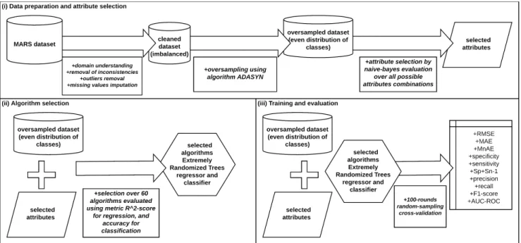
Figure 1: Overview of our methodology, which comprises three stages: (i) data preparation and attribute selection, (ii) algorithm selection, and (iii) training and evaluation.

<15; moderate (class 2) for 15 ≤ AHI < 30; and severe (class 3) for AHI ≥ 30. As we review in Section 2, the performance of OSA diagnosis ranges in between 70% and 80%; that is, it is not a problem easy to solve.

Our results can benefit the development of tools for the auto-matic screening of patients who go through polysomnography and further treatments of OSA. Our thorough methodology enables experimental reproducibility on similar OSA-detection problems, and more generally, on other problems with similar datasets. We review related works in the next section; in Section 3, we detail our dataset, an important factor in this kind of research. Figure 1 illustrates our methodology, which comprises three stages: (i) data preparation and attribute selection, presented in Sections 4 and 5, respectively; (ii) algorithm selection, presented in Section 6; and (iii) training and evaluation, presented in Section 7 along with a comparison to related works. We present further discussion in Section 8, and Section 9 concludes the paper.

2

RELATED WORK

We consider state-of-the-art approaches that investigate the task of predicting the presence or the severity of Obstructive Sleep Apnea based on factors other than the polysomnography-based Apnea-Hypopnea Index (AHI).

The work of Ustun et al. [21] discusses OSA prediction based on clinical indicators before employing their method named Su-persparse Linear Integer Model (SLIM). This method aims to find a simple arithmetic scoring questionnaire to be carried on paper; the score is used as an indicator of a clinical condition of interest. Although the results are not comparably sound to other more elab-orated works, the authors elegantly demonstrated that OSA is to be diagnosed by means of easier-to-acquire factors.

In the work of Wu et al. [25], the authors use a neural fuzzy evalu-ation system [26] over 17 patient variables to predict the occurrence of OSA, as well as the value of indicator AHI. Their findings, by means of a stepwise regression [3], indicate that variables Body Mass Index (BMI), difference of systolic blood pressure before go-ing to sleep and early in the morngo-ing, and the Epworth Sleepiness Scale (ESS) [1], were the most important factors in predicting OSA. Their work was based on 150 patients. Our work uses one order of magnitude more patients.

Mencar et al. [15] perform an extensive investigation of the ap-plicability of ML methods to detect OSA. They use 8 classification strategies and 6 regressions over 19 variables; they found that Sup-port Vector Machine [20] and Random Forest models [4] work best for classification, while Support Vector Machine and Linear Re-gression [19] are most effective on predicting the AHI value. They also demonstrated that a limited number of variables is enough for such tasks. Their work was based on 313 patients. Our work uses one order of magnitude more patients. Moreover, they do not investigate the ample set of ML algorithms that we use.

More recently, Huang et al. [12] conducted a robust investigation of over 6,875 individuals using Support Vector Machines. Their results are convincing and widely discussed with abundant evidence. However, the applicability of their work is limited. The authors used the AHI in data modeling and preparation. To achieve high performance, they partitioned data according to gender, age, and AHI, which resulted in a different model for each partition; each model relying on a different set of variables. Despite the fact that this methodology can reveal important facts, it is not usable in a real scenario because, initially, one does not have the AHI value.

It interesting to note that each work considers a different set of variables; they vary in number and type. This is possibly due to the

specific medical routine that originated each work. As we discuss in Section 8, this fact and the use of proprietary datasets do not permit an absolute comparison among different works. We address this issue by detailing and comparing the steps of our methodology.

3

THE MARS DATASET

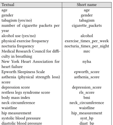
We use a dataset named MARS, provided by the Centre Hospitalier Universitaire of the city of Grenoble, France. The dataset comprises of 1,042 patients, each one depicting 20 features including age, gender, smoking, (yes/no), number of cigarette packets per year, alcohol use (yes/no), physical exercise frequency (weekly), nocturia frequency (urination at night), Medical Research Council scale for the difficulty in breathing, New York Heart Association for heart failure, Epworth Sleepiness Scale, asthenia (physical strength loss) score, depression score, restless legs syndrome score, body mass index, neck circumference (cervical perimeter), waistline (abdomi-nal perimeter), hip measurement, systolic blood pressure, diastolic blood pressure, and cardiac frequency. All of them are measurable without complex exams in comparison to the expensive and time-consuming polysomnography. Table 1 summarizes the features and their short names used throughout the paper.

Textual Short name

age age

gender gender

tabagism (yes/no) tabagism number of cigarette packets per

year

cigarette_packets

alcohol use (yes/no) alcohol physical exercise frequency exercise_times_per_week nocturia frequency nocturia_times_per_night Medical Research Council for

diffi-culty in breathing

mrc

New York Heart Association for heart failure

nyha

Epworth Sleepiness Scale epworth_score asthenia (physical strength loss)

score

asthenia_score

depression score depression_score restless legs syndrome score rls_score body mass index bmi neck circumference neck_circumference

waistline waistline

hip measurement hip_measurement systolic blood pressure syst_bp diastolic blood pressure diast_bp

Table 1: Set of attributes in the dataset MARS along with their short version used throughout the text.

For this investigation, we consider polysomnography results in an attended setting (sleep laboratory) as the “gold standard” for the diagnosis of OSA. Among the measures acquired by a polysomnog-raphy session, the most important is the Apnea-Hypopnea Index (AHI). Hence, all of the records of our dataset include a continuous AHI value that ranges from 0 to 141. The AHI is defined as the

average sum of apneas and hypopneas per hour of sleep; apnea is defined as the absence of airflow for more than 10 seconds; and hypopnea corresponds to a reduction in the respiratory effort with more than 4% oxygen desaturation. The value of the AHI in adults points to four classes of OSA: an AHI < 5 events per hour is con-sidered normal (class 0); mild (class 1) for 5 ≤ AHI < 15; moderate (class 2) for 15 ≤ AHI < 30; and severe (class 3) for AHI ≥ 30. This referential allows the application of two ML tasks: (i) prediction of the AHI continuous value for a given patient; (ii) classification of a patient into one of the four classes of OSA. For patients positively diagnosed (AHI > 5), continuous positive airway pressure (CPAP) therapy is the recommended treatment.

From Figure 2(a), one can see that MARS consists mostly of OSA-positive cases (AHI ≥ 5), notably of severe cases (AHI ≥ 30). The data distribution indicates that the patients who look for OSA screening already have a diagnosis suspicion. This reveals that the dataset is severely imbalanced – see Figure 2(b), showing that only 6.5% of patients have a normal status (non-OSA).

Figure 2: AHI distributions in the MARS dataset. (a) Distri-bution of the AHI continuous values. (b) DistriDistri-bution of the OSA classes based on the AHI value.

4

DATA PREPARATION

MARS is a real-world generated dataset used in a production set-ting. As such, it includes inconsistent values, missing values, and imbalance. These problems directly impact the use of MARS and had to be treated beforehand.

Inconsistent values

For treating inconsistent values, we drew boxplots [23] considering all fields, from which we identified patients having attributes whose values are far from the interquartile range (IQR) and its lower and upper 1.5 whiskers. We also found patients with negative age values and null polysomnography exams. Accordingly, our first data preparation was to exclude all these records because they could not be fixed and had the potential to jeopardize the learning of our algorithms.

Missing values

We learned that the majority of records had at least one missing value. This occurred for as many as 20 attributes. This was possibly because the very patient did not know the value or because the annotation was faulty. While null values are not necessarily a threat to learning data patterns, many ML algorithms simply cannot oper-ate in such circumstances due to numeric or algorithmic reasons.

We solved this problem by substituting the missing values of each field by its median value. The reason is that: (i) none of the fields data distribution was clearly Gaussian, hence we could not use the mean value; (ii) the algorithms we use are based on Naive Bayes and Decision Trees, which are barely affected by the median value as it provides little or no information for a given patient with respect to the upper and lower 50% of the data.

Imbalance

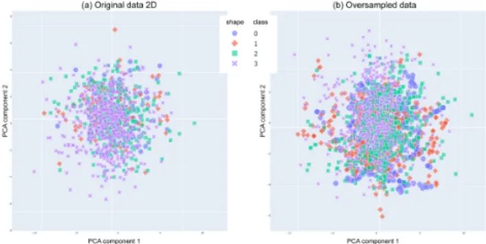
As we discussed in Section 3, the data is heavily skewed to cases with higher severity. The impact of this imbalance is that the ML algorithms are not able to correctly learn which regions of the space refer to which classes. As we can see in Figure 3(a), although the samples of class 3 (severe) patients are concentrated in a specific central region, there are samples of class 3 scattered all over. Many samples of class 3 can be considered as outliers (located away from the denser cluster) that occupy odd regions of the space, yet, they outnumber other classes due to the strong imbalance. As a result, during our initial experiments, our algorithms reported that all the test samples belonged to class 3.

Figure 3: Principal Component Analysis 2D scatter plot visu-alization. (a) Original data. (b) Data oversampled with tech-nique ADASYN [11].

To alleviate this problem, we applied oversampling technique ADASYN [11], an improved version of method SMOTE. This method works by identifying the hard-to-classify samples of the minority class by means of a k-NN neighborhood inspection (we use k=5 and Euclidean distance); the samples of interest are the ones with the highest ratio of 𝑘 nearest neighbors belonging to a different class. It then generates synthetic points in the proximity of these samples by linearly interpolating data; the interpolation considers a sample of interest and its closest neighbors of the same class, creating synthetic data in the space between them. Given two samples 𝑥𝑖

and 𝑥𝑧𝑖, the new synthetic data point is given by:

𝑠𝑖= 𝑥𝑖+ (𝑥𝑧𝑖− 𝑥𝑖) ∗ 𝜆 (1)

where 𝜆 ∈ [0, 1] is a random number. As its authors point out, ADASYN adaptively shifts the classification decision boundary toward the difficult examples. In Table 2, we present the origi-nal cardiorigi-nality of the data and the oversampled cardiorigi-nality after ADASYN.

Class Original Oversampled

0 68 561

1 115 565

2 293 566

3 566 570

Total 1,042 2,262

Table 2: Data cardinality, before and after oversampling.

Figure 3(b) presents the Principal Component Analysis scatter plot visualization after oversampling with ADASYN. The visual-ization shows that many regions populated by class 0 and class 1 samples became more densely populated with samples of these classes. This is particularly true in the periphery of the space. In the central part of the space, one can see that classes 0 and 1 are still hard to separate, which constitutes a challenge for the algorithms.

Class Precision Recall F1-score Support

Original normal 0.00 0.00 0.00 17 mild 0.23 0.17 0.20 29 moderate 0.32 0.23 0.27 73 severe 0.57 0.74 0.64 142 O v ersample d _{normal 0.44 0.64 0.52 143} mild 0.35 0.39 0.37 140 moderate 0.38 0.23 0.29 141 severe 0.54 0.42 0.47 142 Table 3: Effects of oversampling given by precision and re-call of the standard Naive-Bayes algorithm – original versus oversampled data, using 75% for train and 25% for testing over 100-rounds stratified sampling.

Table 3 depicts the effects of oversampling using the standard Naive-Bayes algorithm (refer to Section 5). Before oversampling (“Original”), normal-class patients could not be detected during test-ing. This is because their space was populated with outliers from the other classes; as a result, that space was interpreted as char-acterizing classes 2 (moderate) and 3 (severe). After oversampling (“Oversampled”), the misinterpreted regions of the space charac-terized the minority classes (normal and mild) – this new setting obviously reduced the recall of the majority class (severe), but now we can detect normal patients, and more mild patients. Nevertheless, the Precision regarding the majority classes was barely impacted, which indicates that the learning algorithm was able to absorb the new information without “forgetting” the original setting, see Table 3, 1st column, rows 5 and 9.

5

ATTRIBUTE SELECTION

In Section 3, we saw that the original data comprises 20 variables. We observed that most of them are of little use in the ML pro-cess. This is because some of them are correlated, noisy, ineffective for decision making, or simply non-relevant for the problem at hand. Besides, this large number of variables demands excessive processing time. To find which variables were the most relevant to our problem, we used a Naive-Bayes classifier [17] to experi-ment with all possible attribute combinations. That is, we trained

and validated the classifier over all theÍ20 𝑘=1

20!

𝑘!∗(20−𝑘)! =1,048,575

possible attribute combinations. For each round, we used a 5-fold cross-validation, averaging the one-versus-the-rest Area Under the Receiver-Operating Characteristic (AUC-ROC) performance results with respect to the predicted class of the patients.

We used the classifier provided by the Scikit-Learn library1. It implements the standard algorithm which draws the distributions of each variable and computes the conditional probability 𝑃 (𝑦𝑖|𝑥𝑖).

In our case, for each sample validation, the algorithm computes 𝑃(𝑦_𝑖 = 𝑐𝑙𝑎𝑠𝑠 |𝑥_𝑖 = {𝑠𝑒𝑡 𝑜 𝑓 𝑎𝑡𝑡𝑟𝑖𝑏𝑢𝑡𝑒𝑠 𝑣𝑎𝑙𝑢𝑒𝑠 }). Once the probability is computed, we calculate the ROC curve by varying the classifi-cation threshold for each class. We opted for Naive Bayes because it depends on data distributions, it is interpretable, it is known for providing accurate results [18], and because it has low computing cost.

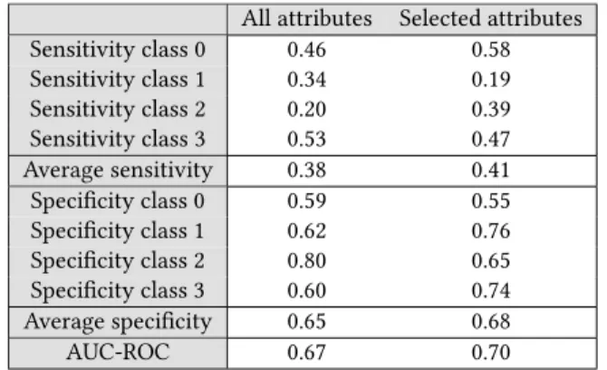
We performed the processing twice, which produced slightly different results due to the data shuffling. The final set of attributes corresponds to the set intersection of the results of the two ma-chines: age, smoking, nocturia frequency, depression score, body mass index, neck circumference, hip measurement, and diastolic blood pressure. Table 4 presents the results for Naive-Bayes. The results show improvements in both sensitivity and specificity when using the selected attributes.

All attributes Selected attributes Sensitivity class 0 0.46 0.58 Sensitivity class 1 0.34 0.19 Sensitivity class 2 0.20 0.39 Sensitivity class 3 0.53 0.47 Average sensitivity 0.38 0.41 Specificity class 0 0.59 0.55 Specificity class 1 0.62 0.76 Specificity class 2 0.80 0.65 Specificity class 3 0.60 0.74 Average specificity 0.65 0.68 AUC-ROC 0.67 0.70

Table 4: Detection of classes using Naive-Bayes in terms of sensitivity and specificity (one versus the rest) for all the at-tributes, and for the selected attributes.

Discussion on the selected attributes

We selected the attributes based on strong experimental evidence. Yet, gender, which is a variable pointed out as important in other works, was not selected in our procedure – see Table 5. For instance, gender appears as important in the works of Mencar et al. [15] and Ustun et al. [21], but not in our setting. Possibly, this is because females are under-represented in our work, and in the works of Wu et al. [25] and Huang et al. [12]; in our dataset, only 26% of the patients are women.

Features related to the patient’s age and weight (body mass index, waistline, neck circumference, and/or hip measurement) are attributes of choice in all the related works – definitely, obesity is

1_{https://scikit-learn.org/stable/modules/naive_bayes.html}

relevant to the detection of OSA [22]. This fact is revealing and, at the same time, it demonstrates the complexity of the problem; this is because not every patient with OSA is obese. One question that might be worth pursuing in a future work is: which factors cause patients with low bmi to develop OSA?

Still looking at Table 5, the presence of blood-pressure-related features is noticeable, but less straightforward; these features ap-pear in three of the five works (including ours). It is easy to find work [14] that states a strong correlation between obesity and hy-pertension (also diabetes), and between OSA and hyhy-pertension [8]. Therefore, while obesity might explain OSA and hypertension, OSA can worsen hypertension issues even further, a relevant discussion, but that is outside the scope of this work – please refer to the work of Wolk et al. [24]. Another relevant feature refers to the Epworth Sleepiness Scale, which points out that daily sleepiness is quite rel-evant – the limitation here is that sleepiness is subjective in nature, and might be caused by other factors other than OSA, reducing the discriminability of this feature [5]. Other non-unanimous features, considering our review, include smoking and nocturia frequency, which seem to have an impact on OSA detection, but that are not fundamental.

Work Selected features

Wu et al. [25] age; body mass index; Epworth Sleepiness Scale; waistline; neck circumference; and difference of blood pressure before going to sleep and early in the morning Mencar et al. [15] body mass index; gender; and Epworth

Sleepiness Scale

Huang et al. [12] age; waistline; neck circumference; snoring; sleep onset latency; and witnessed apnea Ustun et al. [21] age; body mass index; gender; diabetes;

hy-pertension; and tabagism

This work age; nocturia frequency; body mass index; depression score; neck circumference; hip measurement; diastolic blood pressure; and tabagism

Table 5: Selected features after preprocessing in the state-of-the-art works.

6

CHOOSING AN ALGORITHM

The automatic detection of Obstructive Sleep Apnea defines two types of problems that depart from the clinical signals (see Table 1) of a given patient: regression or classification. Regression cor-responds to determining the value of the Apnea-Hypopnea Index. Classification corresponds to determining the status of a patient, a 4-classes problem (normal, mild, moderate, or severe). For the two tasks, we benefit from the advanced and matured frameworks available in the Scikit-Learn ecosystem (https://scikit-learn.org/); accordingly, we experimented with 60 regression and classification algorithms to find the most effective solutions – see Table 6.

Regression Classification Bayesian ARD Ada Boost Bagging Bagging

Bayesian Ridge Bernoulli Naive Bayes Elastic Net Calibrated CV Elastic Net CV Decision Tree Extra Trees Extra Tree Gradient Boosting Extra Trees

Hist Gradient Boosting Gaussian Naive Bayes K-Neighbors Gaussian Process Lars Gradient Boosting Lars CV Hist Gradient Boosting Lasso K-Neighbors

Lasso CV Label Propagation Lasso Lars Label Spreading

Lasso Lars CV Linear Discriminant Analysis Lasso Lars IC Linear Support Vector Linear Logistic Regression Linear Support Vector Logistic Regression CV Multi-layer Perceptron Multi-layer Perceptron Nu Support Vector Multinomial Naive Bayes Partial Least Squares Nearest Centroid Random Forest Nu Support Vector Ridge Passive Aggressive Ridge CV Perceptron

Stochastic Gradient Descent Quadratic Discriminant Analysis Support Vector Machine Random Forest

Theil-Sen Ridge Transformed Target Ridge CV XGBoost Stacking

Stochastic Gradient Descent Support Vector Machine XGBoost

Table 6: Lists of the regression and classification algorithms experimented over dataset MARS.

6.1

Regression problem

For regression, we experiment with 28 different algorithms as de-tailed in Table 6. Figure 4 presents the 𝑅2-score (or coefficient of determination) computed with each of the available regressors over the MARS dataset, using default parameters and the selected attributes presented in Section 5. We compute the performance over a 33%-split validation set, iterating up to 300 times depending on the algorithm. The regressors are ordered according to their score, the best ones with a higher score to the right. One can see that regressors HistGradientBoosting, and ExtraTrees had the best performances.

6.2

Classification problem

For classification, we experiment with 32 different algorithms as detailed in the Appendix. Figure 5 presents the accuracy score computed with each of the available classifiers over MARS, using default parameters and the selected attributes in Section 5. Similarly to the experiments with regressors, we compute the performance

Figure 4: Comparative 𝑅2-score plot of all the 41 regressors using default parameters over dataset MARS.

over a 33%-split validation set, iterating up to 300 times. In the figure, the classifiers are ordered according to their score; the best performances were achieved with algorithms RandomForest and ExtraTrees.

Figure 5: Comparative accuracy plot of all the 32 classifiers using default parameters over dataset MARS.

Algorithm of choice

Considering the performance for both regression and classification, after experimenting with 60 algorithmic configurations, we pro-ceed using algorithm ExtraTrees (Extremely Randomized Trees [9]). Extremely Randomized Trees refer to an ensemble algorithm quite similar to the popular Random Forests [4]. The principle is to use a bagging technique, that is, to pick multiple sets of random samples from the data (with replacement), each one using a subset of the original features; then, a decision tree is built for each set; the final classification is given by majority voting. Extremely Randomized Trees differ from Random Forests in two aspects: the algorithm does not use bagging but a single dataset; each tree builds on random splits rather than on using the “best split” according to a metric such as the Gini Impurity [4]. Both algorithms build hundreds of trees; we experimented with 150, after empirical testing.

The use of Extremely Randomized Trees is known to work better in the presence of noisy attributes, that is, attributes that do not add

This work Huang et al. [12] Mencar et al. [15] Wu et al. [25] Ustun et al. [21] Meta data Cardinality (#patients) 1,042 6,875 313 150 1,922 Number of methods/models 60 5 12 6 2

Source code available Yes No No No No Data preprocessing

Outliers removal Yes No No No Yes Data imputation Yes No No No No Synthetic data generation Yes No Yes No No

AHI Regression

Root meansquared error (RMSE) 16.25 - - 16.61 -Mean absolute error (MAE) 9.6 - - - -Median absolute error (MnAE) 4.15 - - -

-OSA-severity classification Specificity (Sp) 0.83 0.71 - 0.75 0.77 Sensitivity (Sn) 0.64 0.73 - 0.77 0.64 Sp+Sn-1 0.48 0.44 - 0.52 0.41 Precision 0.67 - 0.40 - -Recall 0.68 - 0.45 - -F1-Score 0.66 - 0.41 - -AUC-ROC 0.85 0.80 0.65 - 0.785

Table 7: Comparison to related works. Metrics obtained with algorithm Extremely Randomized Trees set with 150 estimators and evaluated with 100 rounds of random stratified-sampling cross-validation, each round with 66% of the data for training and 33% for validation.

value to the algorithmic decision. Hence, having our experiments recommend the use of Extremely Randomized Trees is a signal that our dataset is significantly noisy; however, this recommendation is not necessarily ideal for other OSA risk-prediction datasets. Instead, our recommendation is to perform the same algorithmic massive evaluation to find which regressor and classifier work better – ac-cordingly, we make the source code that performs this evaluation available at https://github.com/jfrjunio/OSAML.

6.3

Evaluation metrics

Each kind of problem demands specific evaluation metrics. In the case of regression, we use root mean squared error (RMSE), mean absolute error (MAE), and median absolute error (MAE). For clas-sification, we use precision, sensitivity/recall, specificity, F1-score, and AUC-ROC. In the case of classification, the binary metrics are computed for each class versus the others, after which we average the results for each class. With these sets of metrics, it is possible to compare our work to all the works presented in Section 2.

7

COMPARISON TO RELATED WORKS

Table 7 summarizes our comparison to the related work. Unfortu-nately, we are not able to experiment on the same datasets as they are proprietary and inaccessible. For this reason, besides the metrics usually used for performance in regression and classification, we use other dimensions related to the whole process, in particular to data preparation. This contributes to an improved methodology overall and a more comprehensive evaluation.

In Table 7, one can see that our results are superior or comparable to all of the former works with respect to regression and classifi-cation metrics using the attributes selected in Section 5 over Ex-tremely Randomized Trees, as explained in Section 6. We computed the metrics using 100 rounds of random stratified-sampling cross-validation, each round with 66% of the data for training and 33% for validation (oversampled dataset). With respect to the steps of the methodology, our work is more extensive; this is especially true for the number of methods used to find the best models for regression and classification. As reported in Section 6, we experimented with 28 regression algorithms, and 32 classification algorithms.

8

DISCUSSION ON OUR CONTRIBUTION

Concerning the data preparation, although our pre-processing steps are not new, we believe we put together a comprehensive set of techniques: distribution analysis, box-plot-based outlier detection and elimination, imputation of missing values, synthetic data gen-eration, and principal component visual analysis. The attribute selection process, in turn, was performed over a procedure with results potentially more precise than those of other works because it was carried exhaustively to find the best set of attributes. Nev-ertheless, we warn that a larger and more diversified dataset is likely to yield more universal conclusions. This is an open issue for OSA-detection in general.

Despite our good results presented in Section 7, the absence of a benchmark does not permit experimentation in the same conditions, preventing the extrapolation of our conclusions. Hence, as we report in Table 7 and demonstrate in Section 6, instead of advocating

for a specific method, we experimented with the largest set of possible approaches. We also provide numbers on the efficacy of each possible solution both for regression and classification. This amplitude is the strongest point of our work; with this thorough experimentation, we provide a versatile methodology on how to solve OSA risk-prediction problems, including the source code for this project, available at https://github.com/jfrjunio/OSAML. Overall, our data analysis and ML processes can guide not only the OSA-detection problem, but also tasks that rely on datasets with a similar model and goal.

As a last remark, we reflect on a critical aspect common to all the reviewed works, including ours: the limited data size. The largest one presented in [12] reports a study involving 6,875 patients. None of the existing works explicitly includes attributes such as ethnic diversity and gender under-representation, which have long been considered as a determinant in medicine [7]. This fact is to be taken into account not only with respect to our work, but to all the works reviewed so far.

9

CONCLUSIONS

We described the process of using ML in the task of automated Obstructive Sleep Apnea (OSA). We used the MARS dataset from the Centre Hospitalier Universitaire of the city of Grenoble, France, which comprises 1,042 patients diagnosed with all the four levels of OSA severity. In our analysis, we found that the dataset was challenging due to its complexity, missing values, extreme class im-balance, large number of attributes, and due to the fact that patients with normal diagnostic (non-OSA) were not categorically different from those with severe OSA problems. The solution was two-fold, including an extensive dataset pre-processing, and a robust algo-rithm selection. We tuned the dataset using oversampling, reducing the detection of positive OSA patients, but increasing the detection of normal non-OSA patients as measured by sensitivity, specificity, precision, recall, f1-measure, and AUC-ROC. For attribute selection, we experimented with 60 algorithms (28 regressors and 32 classi-fiers). The verdict was to use Extremely Randomized Trees, which are tailored to noisy data. As for our contribution, we follow our methodology for data preparation and algorithm selection since each dataset presents its peculiarities even for the same problem.

We also investigated the most important attributes for OSA de-tection, which included recurrent factors of age, weight, blood pressure, and sleepiness-related measures. We compared them to the selected features indicated in the related work. For our dataset in particular, the features of nocturia and depression played a rel-evant role. However, we warn the reader that each dataset has its characteristics and a corresponding set of features. Further in-vestigation is required on such diversity. Finally, we suggest the need for a more robust and diversified dataset because the ones used in this and other works are rather small in the number of patients, not systematically covering ethnic diversity and gender representativeness.

ACKNOWLEDGMENTS

This research was financed by French agency Multidisciplinary Institute in Artificial Intelligence (Grenoble Alpes, ANR-19-P3IA-0003); and by Brazilian agencies Fundacao de Amparo a Pesquisa do

Estado de Sao Paulo (2018/17620-5, and 2016/17078-0); Conselho Na-cional de Desenvolvimento Cientifico e Tecnologico (406550/2018-2, and 305580/2017-5); and Coordenacao de Aperfeicoamento de Pes-soal de Nivel Superior (CAPES, Finance Code 001). We thank NVidia for donating the GPUs that supported this work.

REFERENCES

[1] Abrishami, A., Khajehdehi, A., and Chung, F. (2010). A systematic review of screening questionnaires for obstructive sleep apnea. Canadian Journal of Anesthe-sia/Journal canadien d’anesthésie, 57(5):423–438.

[2] AlGhanim, N., Comondore, V. R., Fleetham, J., Marra, C. A., and Ayas, N. T. (2008). The economic impact of obstructive sleep apnea. Lung, 186(1):7–12.

[3] Armitage, P., Berry, G., and Matthews, J. (2002). Modelling continuous data. Statistical methods in medical research, pages 312–377.

[4] Breiman, L. (2001). Random forests. Machine learning, 45(1):5–32.

[5] Chervin, R. D. and Aldrich, M. S. (1999). The epworth sleepiness scale may not reflect objective measures of sleepiness or sleep apnea. Neurology, 52(1):125–125. [6] Chung, F., Yegneswaran, B., Liao, P., Chung, S. A., Vairavanathan, S., Islam, S.,

Khajehdehi, A., and Shapiro, C. M. (2008). Validation of the berlin questionnaire and american society of anesthesiologists checklist as screening tools for obstructive sleep apnea in surgical patients. Anesthesiology: The Journal of the American Society of Anesthesiologists, 108(5):822–830.

[7] Cruickshank, J. K. and Beevers, D. G. (2013). Ethnic factors in health and disease. Butterworth-Heinemann.

[8] Dopp, J. M., Reichmuth, K. J., and Morgan, B. J. (2007). Obstructive sleep apnea and hypertension: Mechanisms, evaluation, and management. Current Hypertension Reports, 9(6):529–534.

[9] Geurts, P., Ernst, D., and Wehenkel, L. (2006). Extremely randomized trees. Machine learning, 63(1):3–42.

[10] Gilat, H., Vinker, S., Buda, I., Soudry, E., Shani, M., and Bachar, G. (2014). Ob-structive sleep apnea and cardiovascular comorbidities: a large epidemiologic study. Medicine, 93(9).

[11] He, H., Bai, Y., Garcia, E. A., and Li, S. (2008). Adasyn: Adaptive synthetic sampling approach for imbalanced learning. In IEEE world congress on computational intelligence, pages 1322–1328.

[12] Huang, W. C., Lee, P. L., Liu, Y. T., Chiang, A. A., and Lai, F. (2020). Support vector machine prediction of obstructive sleep apnea in a large-scale Chinese clinical sample. Sleep, 43(7).

[13] Jennum, P. and Riha, R. L. (2009). Epidemiology of sleep apnoea/hypopnoea syndrome and sleep-disordered breathing. European Respiratory Journal, 33(4):907– 914.

[14] Jiang, S.-Z., Lu, W., Zong, X.-F., Ruan, H.-Y., and Liu, Y. (2016). Obesity and hypertension. Experimental and Therapeutic Medicine, 12(4):2395–2399.

[15] Mencar, C., Gallo, C., Mantero, M., Tarsia, P., Carpagnano, G. E., Barbaro, M. P. F., and Lacedonia, D. (2019). Application of machine learning to predict obstructive sleep apnea syndrome severity. Health Informatics Journal, 26(1):298–317. [16] Network, U. H. The official stop-bang questionnaire website. accessed, June/2020. [17] Ren, J., Lee, S. D., Chen, X., Kao, B., Cheng, R., and Cheung, D. (2009). Naive bayes classification of uncertain data. In IEEE Int. Conference on DM, pages 944–949. [18] Saritas, M. M. and Yasar, A. (2019). Performance analysis of ann and naive bayes classification algorithm for data classification. International Journal of Intelligent Systems and Applications in Engineering, 7(2):88–91.

[19] Seber, G. A. and Lee, A. J. (2012). Linear regression analysis, volume 329. John Wiley & Sons.

[20] Steinwart, I. and Christmann, A. (2008). Support vector machines. Springer Science & Business Media.

[21] Ustun, B., Westover, M. B., Rudin, C., and Bianchi, M. T. (2016). Clinical prediction models for sleep apnea: the importance of medical history over symptoms. Journal of Clinical Sleep Medicine, 12(2):161.

[22] Vgontzas, A. N., Tan, T. L., Bixler, E. O., Martin, L. F., Shubert, D., and Kales, A. (1994). Sleep apnea and sleep disruption in obese patients. Archives of internal medicine, 154(15):1705–1711.

[23] Wickham, H. and Stryjewski, L. (2011). 40 years of boxplots. Am. Statistician. [24] Wolk, R., Shamsuzzaman, A. S., and Somers, V. K. (2003). Obesity, sleep apnea,

and hypertension. Hypertension, 42(6):1067–1074.

[25] Wu, M., Huang, W., Juang, C., Chang, K., Wen, C., Chen, Y., Lin, C., Chen, Y., and Lin, C. (2017). A new method for self-estimation of the severity of obstructive sleep apnea using easily available measurements and neural fuzzy evaluation system. IEEE Journal of Biomedical and Health Informatics, 21(6):1524–1532.

[26] Zhao, W., Li, K., and Irwin, G. W. (2012). A new gradient descent approach for local learning of fuzzy neural models. IEEE Transactions on Fuzzy Systems, 21(1):30–44.