HAL Id: inria-00305998
https://hal.inria.fr/inria-00305998v3
Submitted on 28 Jun 2010
HAL is a multi-disciplinary open access
archive for the deposit and dissemination of
sci-entific research documents, whether they are
pub-lished or not. The documents may come from
teaching and research institutions in France or
abroad, or from public or private research centers.
L’archive ouverte pluridisciplinaire HAL, est
destinée au dépôt et à la diffusion de documents
scientifiques de niveau recherche, publiés ou non,
émanant des établissements d’enseignement et de
recherche français ou étrangers, des laboratoires
publics ou privés.
Formalizing Projective Plane Geometry in Coq
Nicolas Magaud, Julien Narboux, Pascal Schreck
To cite this version:
Nicolas Magaud, Julien Narboux, Pascal Schreck. Formalizing Projective Plane Geometry in Coq.
Post-proceedings of Automated Deduction in Geometry (ADG) 2008, Thomas Sturm, Sep 2008,
Shang-hai, China. pp.141-162, �10.1007/978-3-642-21046-4�. �inria-00305998v3�
Formalizing Projective Plane Geometry in Coq
Nicolas Magaud, Julien Narboux, and Pascal Schreck
LSIIT UMR 7005 CNRS - Université de Strasbourg⋆
Abstract We investigate how projective plane geometry can be formal-ized in a proof assistant such as Coq. Such a formalization increases the reliability of textbook proofs whose details and particular cases are often overlooked and left to the reader as exercises. Projective plane geome-try is described through two different axiom systems which are formally proved equivalent. Usual properties such as decidability of equality of points (and lines) are then proved in a constructive way. The duality principle as well as formal models of projective plane geometry are then studied and implemented in Coq. Finally, we formally prove in Coq that Desargues’ property is independent of the axioms of projective plane geometry.
1
Introduction
This paper deals with formalizing projective plane geometry. Projective plane geometry can be described by a fairly simple set of axioms. However it captures the main aspects of plane geometry, especially perspective. It is a good candidate to be formalized in a proof assistant. Most of the description and proofs are available in textbooks such as [8, 3]. However, in most books, many lemmas are considered trivial and many proofs are left to the reader. Building a formal development in a proof assistant allows for more flexibility. If required, axioms can be changed easily and proofs can be rechecked automatically by the system. Such changes may only require minor rewriting of the proofs by the user. In all cases, the proofs are computer-verified, which dramatically increases their reliability compared to paper-and-pencil proofs.
This formalization is not only interesting in itself. It also allows to evaluate the adequacy of a proof assistant such as Coq to develop a formal theory and to build some models of this theory. More significantly, we formalize projective plane geometry because we are interested in building reliable and robust con-straint solving programs (see [16, 15]). Indeed, in geometric concon-straint solving, handling the numerous particular cases is crucial to ensure robustness. Detect-ing whether a configuration is degenerated or not requires theorem provDetect-ing [29]: which theorems are required and how to prove them is among the issues we want to address. As shown in [21], point-line incidences in the projective plane are sufficient to express usual geometric constraints.
Finally, as computer scientists, we are interested in the effectiveness of proofs in order to extract programs from these proofs. The Coq proof assistant [7, 1]
implements a constructive logic and allows program extraction from constructive proofs. Therefore, it is the perfect tool to carry out a constructive formalization. In this paper, we formalize the theory of projective plane geometry and we build models of this theory. In a subsequent paper [18], we revisit and generalize the axiom system for projective geometry in a at least 3 dimensional setting using flats and ranks and prove Desargues’ property holds in that case.
Related Work Proof assistants have already been used in the context of geometry. The task consisting in mechanizing Hilbert’s Grundlagen der Geometrie has been partially achieved. A first formalization using the Coq proof assistant was pro-posed by Christophe Dehlinger, Jean-François Dufourd and Pascal Schreck [10]. This first approach was realized in an intuitionist setting, and concluded that the decidability of point equality and collinearity is necessary to check Hilbert’s proofs. Another formalization using the Isabelle/Isar proof assistant [26] was performed by Jacques Fleuriot and Laura Meikle [19]. Both formalizations have concluded that, even if Hilbert has done some pioneering work about formal systems, his proofs are in fact not fully formal, in particular degenerated cases are often implicit in the presentation of Hilbert. The proofs can be made more rigorous by machine assistance. Frédérique Guilhot realized a large Coq devel-opment about Euclidean geometry following a presentation suitable for use in french high-school [13]. In [24, 25], Julien Narboux presented the formalization and implementation in the Coq proof assistant of the area decision procedure of Chou, Gao and Zhang [5] and a formalization of foundations of Euclidean geometry based on Tarski’s axiom system [33, 30]. In [11], Jean Duprat proposes the formalization in Coq of an axiom system for compass and ruler geometry. Regarding formal proofs of algorithms in the field of computational geometry, we can cite David Pichardie and Yves Bertot [27] for their formalization of convex hulls algorithms in Coq as well as Laura Meikle and Jacques Fleuriot [20] for theirs in a Hoare-like framework in Isabelle. Several papers introduce methods for automatic proof in projective geometry, e.g. [28, 17]. Our work is different because we perform interactive proofs in projective geometry. Our approach is only slightly automated, but we can deal with the degenerated cases by careful study in the proof assistant whereas these cases are ignored in [28]. In addition we can deal with theorems which are not stated as a geometric construction, which is a limitation of approaches based on the Wu’s method and the area method.
Notations Naming/Writing conventions follow the guidelines edited in a recent document proposed by Duprat, Guilhot and Narboux [12]. Most Coq notations, which are really close to mathematical ones, will be explained along the course of the paper. The negation is noted ˜. The most awkward notation for the reader not accustomed to Coq is the curly-brackets notation for constructive existential quantification over the sort Type. For instance, the formula forall l:Line, {X:Point | ˜Incid X l}expresses that ∀l : Line, ∃X : P oint, ¬ Incid X l.
Axiom Line Existence
∀A B : P oint, (∃l : Line, A ∈ l ∧ B ∈ l) Axiom Point Existence
∀l m : Line, (∃A : P oint, A ∈ l ∧ A ∈ m) Axiom Line Uniqueness
∀A B : P oint, A 6= B ⇒ ∀l m : Line, A ∈ l ∧ B ∈ l ∧ A ∈ m ∧ B ∈ m ⇒ l = m Axiom Point Uniqueness
∀l m : Line, l 6= m ⇒ ∀A B : P oint, A ∈ l ∧ A ∈ m ∧ B ∈ l ∧ B ∈ m ⇒ A = B Definition (distinct4)
distinct4 A B C D ≡ A 6= B ∧ A 6= C ∧ A 6= D ∧ B 6= C ∧ B 6= D ∧ C 6= D Axiom Four Points
∃A : P oint, ∃B : P oint, ∃C : P oint, ∃D : P oint, distinct4 A B C D ∧ (∀l : Line, (A ∈ l ∧ B ∈ l ⇒ C /∈l ∧ D /∈l)∧ (A ∈ l ∧ C ∈ l ⇒ B /∈l ∧ D /∈l)∧ (A ∈ l ∧ D ∈ l ⇒ B /∈l ∧ C /∈l)∧ (B ∈ l ∧ C ∈ l ⇒ A /∈l ∧ D /∈l)∧ (B ∈ l ∧ D ∈ l ⇒ A /∈l ∧ C /∈l)∧ (C ∈ l ∧ D ∈ l ⇒ A /∈l ∧ B /∈l))
Figure 1. A first axiomatization of projective plane geometry.
Outline The paper is organized as follows. In section 2, we present the axioms for projective plane geometry and their description in the Coq proof assistant. In section 3, we study the duality between points and lines. Section 4 deals with finite and infinite models for projective plane geometry. In Section 5 we build both desarguesian and non-desarguesian models.
2
Axioms
2.1 A First Set of Axioms
We assume that we have two kinds of objects which we call points and lines. We also assume that we have a relation (∈) between elements of these two sets. We can describe projective plane geometry using the axioms presented in Figure 1. The first two axioms deal with existence of points and lines. We choose not to require points (resp. lines) to be distinct in axiom ’Line Existence’ (resp. ’Point Existence’). If the points (resp. lines) are equal, the line (resp. the point) still
exists: actually there potentially exists an infinity of lines (resp. points). This design choice follows a general rule in formal geometry: it is crucial to consider statements which are as general as possible.
The next two axioms deal with uniqueness of the above defined line and point. These axioms hold only if the two points (resp. lines) are distinct. As suggested in [2], axioms ’Point Uniqueness’ and ’Line Uniqueness’ can be merged into a more convenient axiom with no negation. This axiom is classically equivalent to the conjunction of the two others:
Axiom Uniqueness
∀A B : P oint, ∀l m : Line,
A ∈ l ⇒ B ∈ l ⇒ A ∈ m ⇒ B ∈ m ⇒ A = B ∨ l = m
Finally, axiom ’Four points’ states that there exists at least four distinct points, no three of them being collinear. This means dimension is at least 2. Together with axiom ’Point Existence’ which expresses that the dimension is at most 2 (two lines always intersect), it imposes that the dimension of this projective space is exactly 2. The formalization of this axiom system is straight-forward, but from a practical point of view, proofs in most textbooks often use some variants of this system. To ease mechanization of proofs, we formalize the equivalence between these systems.
2.2 Another Axiom System for Projective Plane Geometry
Another Non-degeneracy Axiom Axiom ’Four Points’ states a non-degene-racy condition, namely that the projective space we consider is not reduced to a single line. This can be expressed in another way through two new axioms: Axiom Three Points
∀l : Line, ∃ABC : P oint, (A 6= B ∧ B 6= C ∧ A 6= C) ∧ A ∈ l ∧ B ∈ l ∧ C ∈ l Axiom Lower Dimension
∃l1: Line, ∃l2: Line, l16= l2
The first axiom expresses that each line contains at least three points; the second one states that there exist two distinct lines.
We prove that axiom ’Four points’ can be replaced by axiom ’Three points’ and axiom ’Lower dimension’ in the system defined in the previous section and vice-versa. Both settings share the following axioms: Line Existence, Point Exis-tence, Uniqueness. In mathematics textbooks, the equivalence of these two sets of axioms is usually presented as a remark1
. For instance in [3], the proof is left to the reader. In a proof assistant such as Coq, these proofs have to be made explicit and proving them formally requires some technical work mostly related to handling the numerous configurations of points. The basic principles of the proof are presented in appendix A.
1
2.3 Implementation in Coq
We formalize the previous definitions in the Coq proof assistant [1, 7]. To do so, we take advantage of the modules and functors of Coq. Modules [6] allow to define parameterized theory and to put together types and definitions into a module structure. This enhances the reusability of developments, by providing a formal interface for such a structure. In addition, functors can be used to connect module types to one another.
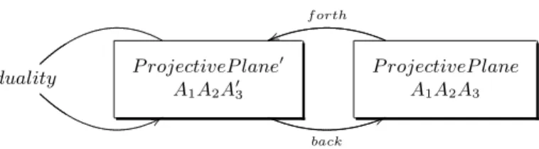
Modules and Projective Plane Our first module PreProjectivePlane con-tains axioms dealing with point (resp. line) existence and uniqueness. From that we derive some basic properties, including uniqueness of a line (resp. of a point), from the general uniqueness axiom. Then, on top of PreProjectivePlane, we build two modules ProjectivePlane which contains axiom ’Four points’ and ProjectivePlane’which contains axiom ’Three points’ and axiom ’Lower di-mension’. A theory is of type ProjectivePlane if it contains all the notions presented in Figure 2 on the following page. The two module types Projective-Plane and ProjectivePlane’ are connected through two functors Back and Forthwhich prove the equivalence of these two axiom systems when the axioms ’Line Existence’ and ’Point Existence’ as well as Uniqueness are available. Figure 2 sums up the module type for projective plane geometry and Figure 3 presents the global organization of the development.
Deciding Equality From the assumption that incidence is decidable, ∀A : P oint, ∀l : Line, (A ∈ l ∨ ¬A ∈ l)
we prove that point (resp. line) equality is decidable. The proofs of decidability for point (resp. line) equality are intuitionist, in the sense that they do not use the excluded middle property. Details of these proofs are available in appendix B. From these basic axioms, we can consider proving some theorems about pro-jective plane geometry. For instance, we prove that if we consider lines as set of points, there always exists a bijection between two lines (see appendix E for details). In order to improve genericity, we show that the well-known princi-ple of duality between point and line can be derived in Coq. It allows us to prove automatically half of the theorems of interest from the proofs of their dual counterparts.
3
Duality
3.1 Principle of Duality
It is well known that projective geometry enjoys a principle of duality, namely that every definition remains significant and every theorem remains true, when
Module Type ProjectivePlane. Parameter Point: Set. Parameter Line: Set.
Parameter Incid : Point -> Line -> Prop.
Axiom incid_dec : forall (A:Point)(l:Line), {Incid A l} + {~Incid A l}. (* Line Existence : any two points lie on a unique Line *)
Axiom a1_exist : forall (A B :Point), {l:Line | Incid A l /\ Incid B l}. (* Point Existence : any two lines meet in a unique point *)
Axiom a2_exist : forall (l1 l2:Line), {A:Point | Incid A l1 /\ Incid A l2}. Axiom uniqueness : forall A B :Point, forall l m : Line,
Incid A l -> Incid B l -> Incid A m -> Incid B m -> A=B \/ l=m.
(* Four points : there exist four points with no three collinear *) Axiom a3: {A:Point & {B :Point & {C:Point & {D :Point |
(forall l :Line, distinct4 A B C D/\
(Incid A l /\ Incid B l -> ~Incid C l /\ ~Incid D l) /\ (Incid A l /\ Incid C l -> ~Incid B l /\ ~Incid D l) /\ (Incid A l /\ Incid D l -> ~Incid C l /\ ~Incid B l) /\ (Incid C l /\ Incid B l -> ~Incid A l /\ ~Incid D l) /\ (Incid D l /\ Incid B l -> ~Incid C l /\ ~Incid A l) /\ (Incid C l /\ Incid D l -> ~Incid B l /\ ~Incid A l))}}}}. End ProjectivePlane.
Figure 2. The module type with axioms required to describe a projective plane. The incidence relation (∈) is noted Incid in our Coq development. {Incid A l} + {˜Incid A l}expresses that we know constructively that A ∈ l ∨ ¬A ∈ l.
we interchange the concepts Point and Line. But as we exchange points and lines, predicates must be exchanged with their dual as well. For example, the collinearity property, i.e. col A B C ≡ ∃l : Line, A ∈ l ∧ B ∈ l ∧ C ∈ l must be replaced by the concurrency property i.e. meet a b c ≡ ∃L : P oint, a ∋ L ∧ b ∋ L ∧ c ∋ L. To formalize this principle, we make use of the module system of Coq [1, 6]. In practice, we consider the module type ProjectivePlane’ defined in the previous section and we build a functor from ProjectivePlane’ to itself in which we map points to lines and lines to points:
Module swap (M: ProjectivePlane’) : ProjectivePlane’. Definition Point := M.Line.
Definition Line := M.Point.
...
To build this functor we need to show that the dual of each axiom holds. It is clear that the axioms of existence and uniqueness of lines are the dual of the axioms for existence and uniqueness of points:
Definition a1_exist := M.a2_exist. Definition a1_unique := M.a2_unique. Definition a2_exist := M.a1_exist. Definition a2_unique := M.a1_unique.
To prove the dual version of axiom ’Three points’ and axiom ’Lower dimen-sion’ it is necessary to use the other axioms. Appendix C provides the detailed proof of the fact that incidence geometry is a dual of itself and Figure 3 a sum-mary of the organization of the development.
3.2 Applications bP duality ⇒ bP1 bP2
Formalizing this principle of duality leads to an interesting theoretical result. In addition, this principle is also useful in practice. For every theorem we prove, we can easily derive its dual using our functor swap. For instance,
from the lemma outsider stating that for every couple of lines, there is a point which is not on these lines, we can derive its dual automatically: for every couple of points, there is a line not going through these points.
Module Example (M’: ProjectivePlane’). Module Swaped := swap M’.
Export M’.
Module Back := back.back Swaped.
Module ProjectivePlaneFacts_m := decidability.decidability Back. Lemma dual_example :
forall P1 P2 : Point,{l : Line | ~ Incid P1 l /\ ~ Incid P2 l}. Proof.
apply ProjectivePlaneFacts_m.outsider. Qed.
End Example.
So far, we focused on axiom systems and formal proofs. The next step is to check whether well-known models verify our axioms for projective plane geom-etry.
duality 8 8 P rojectiveP lane′ A1A2A′3 back 6 6 P rojectiveP lane A1A2A3 f orth v v
Figure 3. A modular organization. Arrows represent functors and boxes represent modules types.
4
Models
In order to prove formally that our sets of axioms are consistent, we build some models. We build both finite and infinite models: among them the smallest pro-jective plane and an infinite model based on homogeneous coordinates.
4.1 Finite Models
Following Coxeter’s notation [8], a finite projective geometry is written P G(a, b) where a is the number of dimensions, and given a point on a line, b is the number of other lines through the point. We build two finite models: P G(2, 2) and P G(2, 5). P G(2, 2) is the smallest projective plane and is also known as Fano’s plane. b A bB b b G bE b F b D bC Fano’s Plane In two dimensions, we can easily build the
model with the least number of points and lines: 7 each. This model is called Fano’s plane. On the figure, points are simply represented by points, whereas lines are represented by six segments and a circle (DEF ).
We define a module FanoPlane of type ProjectivePlane.
The typing system of Coq will ensure that our definitions are really instances of the abstract definition of a projective plane.
The set of points is defined by an inductive2
type with 7 constructors and the set of lines as well:
Inductive ind_point : Set := A | B | C | D | E | F | G.
Inductive ind_line : Set := ABF | BCD | CAE | ADG | BEG | CFG | DEF. Definition point : Set := ind_point.
Definition line : Set := ind_line.
The incidence relation is given explicitly by its graph:
2
Note that this type is not really inductive, but sum types are defined in Coq using a special case of the general concept of inductive types.
Definition incid_bool : Point -> Line -> bool := fun P L => match (P,L) with
(A,ABF) | (A,CAE) | (A,ADG) | (B,BCD) | (B,BEG) | (B,ABF) |(C,BCD) | (C,CAE) | (C,CFG) | (D,BCD) | (D,ADG) | (D,DEF) |(E,CAE) | (E,BEG) | (E,DEF) | (F,ABF) | (F,DEF) | (F,CFG) |(G,ADG) | (G,CFG) | (G,BEG) => true
| _ => false end.
The proofs of existence and uniqueness are performed by case analysis. Note that in order to prove the axioms of uniqueness, we must prove that for every couple of points (resp. lines) there is a unique line (resp. point). This creates 72
= 49 cases. For each of these cases, we have to perform a case analysis on the lines, this produces again 49 cases, leading to a total of 2401 cases. The proof is computed easily by Coq.
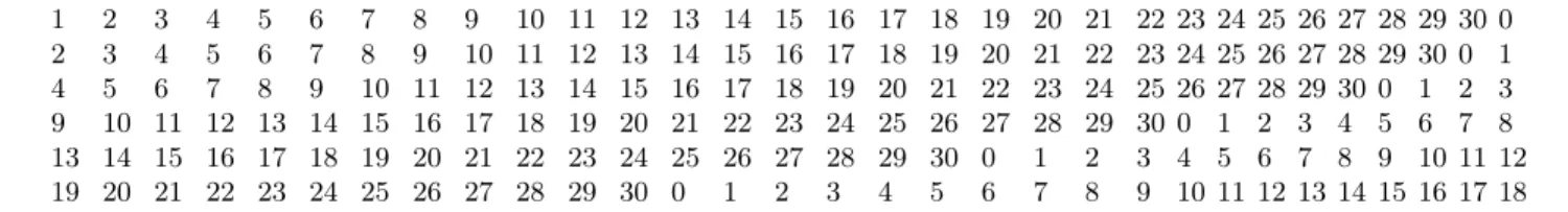
PG(2,5) We follow [8] and build another model of the projective plane which is still finite but larger than Fano’s plane. This model is called P G(2, 5). It contains 31 points and as many lines. The incidence relation is given on table 1 in appendix D. From the technical view of the formalization, this model is harder to build than Fano’s plane because the proof produces 923 521 cases3
. However, the proofs of these cases can be automated. The total size of the proof object generated by Coq (a term of the calculus of inductive constructions) is 7 Mo. 4.2 Infinite Model: Homogeneous Coordinates
To build an infinite model of projective geometry we use homogeneous coordi-nates introduced by August Ferdinand Möbius. We present our formalization in the context of the projective plane, but it can be easily generalized to any other dimension. The homogeneous coordinates of a point (resp. of a line) of a projec-tive plane is a triple of numbers which are not all zero. These numbers are ele-ments of any commutative field of characteristic zero. Two triples which are pro-portional are considered as equal: for any λ 6= 0, (x1, x2, x3) = (λx1, λx2, λx3).
To formalize this notion in Coq it would be natural to define pseudo-points as triple of elements of a field and then define points (resp. lines) as the equivalence classes of proportional non-zero triple in this field. Unfortunately, defining a type by quotient is something difficult to do in the calculus of inductive constructions used by Coq [31]. Therefore, we choose to define the quotient type directly by representing the classes of points and lines by a normal form. Points and lines are represented by their triple of coordinates such that the last non zero
3
In [8], the proof given is the following: “we observe that any two residues are found together in just one column of the table (see on page 20), and that any two columns contain just one common number”. This amounts to checking, for more than 400 different configurations, whether two sets of six elements have only one common element. In such a case, mechanized theorem proving is the best way to ensure correctness.
coordinate is 1. Consider a point (x1, x2, x3). If x3 6= 0 we can represent it by (x1/x3, x2/x3, 1). If x3= 0, we perform case distinction on x2. If x26= 0 we can represent it by (x1/x2, 1, 0), else we represent it by (1, 0, 0). This definition can be formalized in Coq using the following inductive type where F is the type of the elements of our field and P0, P1 and P2 are the constructors for the three different cases:
Inductive Point : Set :=
| P2 : F -> F -> Point (* (x1,x2,1) *) | P1 : F -> Point (* (x1,1 ,0) *) | P0 : Point. (* (1 ,0 ,0) *)
The second and third constructors correspond to ideal points (points at in-finity).
The incidence relation (noted Incid in Coq and ∈ in this paper) can then be defined as the inner product of a point and line. The definition of the inner product can be made more generic by using triples, instead of giving a definition distinguishing each of the 3 × 3 cases.
To do this, we define two functions, one to transform a point into a triple of coordinates, and another one to normalize a triple of coordinates to obtain a point. We can then prove two lemmas which state that our definitions are consistent:
Lemma triple_point :
forall P : Point, point_of_triple (triple_of_point P) = P. Lemma point_triple :
forall a b c : F, (a,b,c) <> (0,0,0) ->
exists l, triple_of_point (point_of_triple (a,b,c)) = (a*l,b*l,c*l). Lemma point_of_triple_functionnal:
forall a b c l : F, (a,b,c) <> (0,0,0) -> l <> 0 -> point_of_triple(a,b,c) = point_of_triple(a*l,b*l,c*l).
The inner product and incidence relations can then be defined as:
Definition inner_product_triple A B := match (A,B) with
((a,b,c),(d,e,f)) => a*d+b*e+c*f end.
Definition Incid : Point -> Line -> Prop := fun P L =>
inner_product_triple (triple_of_point P) (triple_of_line L) = 0.
Now, we need to prove that the axioms of a projective plane hold in this setting. The proof of the decidability of Incid and of axioms (Three Points) and (Lower Dimension) are straightforward. For the uniqueness axiom, after
unfolding of definitions, the problem reduces to a goal involving equations such as the following ones:
r ∗ r5+ r0∗r6+ 1 = 0 r ∗ r3+ r0∗r4+ 1 = 0 r1∗r5+ r2∗r6+ 1 = 0 r1∗r3+ r2∗r4+ 1 = 0
⇒(r = r1∧r0= r2) ∨ (r3= r5∧r4= r6)
Using the following equivalences considered as rewrite rules, we can convert this goal into an ideal-membership problem which can be solved using the Gröb-ner basis tactic developed by Loïc Pottier [9].
∀ab, a = b ⇔ a − b = 0
∀ab, (a = 0 ∨ b = 0) ⇔ ab = 0 ∀ab, (a = 0 ∧ b = 0) ⇔ a2
+ b2 = 0
This tactic provides automation to solve algebraic goals which otherwise would be tedious to prove interactively. Proofs achieved by the Gröbner basis tactic require less than 2 seconds of computation except one which requires about a minute.
Finally, for the existence axioms, we need to define the line passing through two points (resp. the point at the intersection of two lines).
5
Desarguesian and Non-desarguesian Models
Desargues’ property is among the most fundamental properties of projective geometry since in the projective space Desargues’ property becomes a theorem and consequently all the projective spaces arise from a division field. In this section, we formalize two models showing on the one hand, that Desargues’ property is compatible with the axioms of projective geometry and, on the other hand that it is independent of them. Let’s first recall Desargues’ statement in projective geometry.
5.1 Desargues’ Property Desargues’ property states that:
Let E be a projective space and A,B,C,A′,B′,C′ be points in E, if the three lines joining the corresponding vertices of trianglesABC and A′B′C′ all meet in a point O, then the three intersections of pairs of corresponding sides α, β andγ lie on a line.
If E is at least of dimension three, Desargues’ property always holds. In [18], we have formalized this theorem in Coq. If E is of dimension two, Desargues’ property is independent from all the projective plane geometry axioms. We first show that it is not contradictory with these axioms by formally proving it holds in Fano’s plane. Then, we build a model (Moulton’s plane) in which all projective
b A b B b C b O b C’ b A’ b B’ b b b β γ α
plane geometry axioms hold but Desargues’ property does not hold. This is achieved by making explicit a configuration for which Desargues’ property is not satisfied. Overall this shows the independence of Desargues’s theorem from the axioms of projective plane geometry, which can be regarded as the starting point of non-desarguesian geometry [4].
5.2 Fano’s Plane is Desarguesian
At first sight, proving Desargues’ property in Fano’s plane seems to be straight-forward to achieve by case analysis on the 7 points and 7 lines. However, this requires handling numerous cases4
including many configurations which contra-dict the hypotheses.
To formalize the property we make use of two kinds of symmetries, a sym-metry of the theory and a symsym-metry of the statement.
Symmetry of the Statement We first study the special case where the point O of Desargues’ configuration corresponds to A, and the line OA corresponds to ADG, OB to CAE and OC to ADF . Then as Desargues’ statement is symmetric by permutation of the three lines which intersect in O, we can formalize a proof of slightly more general lemma desargues_from_A where the point O of Desargues’ configuration still corresponds to A but the three lines intersecting in O are universally quantified.
Symmetry of the Theory The theory of Fano’s plane is invariant by per-mutation of points. It means that, even if it is not obvious from the figure in section 4.1, all the points play the same role: if (A, B, C, D, E, F, G) is a Fano’s
4
The most naïve approach would consider 77
cases, even with careful analysis it remains untractable to prove all the cases without considering symmetries.
plane then (B, C, D, F, E, G, A) is one as well. We formalize this by building a functor from Fano’s theory to itself which permutes the points. Using this func-tor and desargues_from_A, we show that Desargues’ property holds for any choice for O among the 7 points of the plane.
5.3 Independence of Desargues’ Property
Moulton Plane and its Projective Counterpart Moulton plane [23] is an affine plane in which lines with a negative slope are bent (i.e. the slope is doubled) when they cross the y-axis. It can be easily extended into a projective plane.
Moulton plane is an incidence structure which consists of a set of points P , a set of lines L, and an incidence relation between elements of P and elements of L. Points are denoted by couples (x, y) ∈ R2
. Lines are denoted by (m, b) ∈ (R ∪ ∞) × R (where m is the slope - ∞ for vertical lines - and b the y-intercept). The incidence relation is defined as follows:
(x, y) ∈ (m, b) ⇐⇒ x = b if m = ∞ y = mx + b if m ≥ 0 y = mx + b if m ≤ 0, x ≤ 0 y = 2mx + b if m ≤ 0, x ≥ 0.
This incidence structure verifies the properties of an affine plane. It can be turned into a projective plane through the following process.
– We extend P with points at infinity (one direction point for each possible slope, including the vertical one); therefore P is (R × R) ∪ R.
– We extend the set L of affine lines with a new one which connects all points at the infinite; therefore L is ((R ∪ ∞) × R) ∪ ∞.
– We finally extend the incidence relation in order to have all direction points and only them incident to the infinite line. We also extend each affine line with a direction point (the one bearing its slope).
This construction leads to a projective plane. The whole process is formally described in Coq and we show that all the axioms of projective plane geometry presented in section 2 hold. Most proofs on real numbers rely on using Gröbner basis computation in Coq as already used in section 4.2.
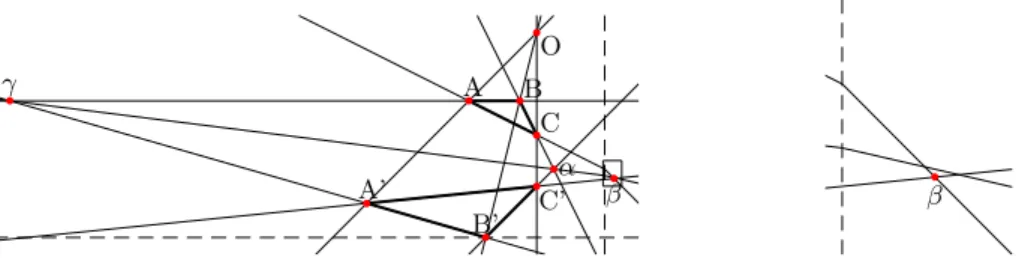
A Configuration of Desargues where the Theorem Does Not Hold We build a special configuration of Desargues for which the property does not hold. This can be achieved in a very algebraic point of view using only coordinates and equations for lines. We first present it that way and then show on a figure why Desargues’ property does not hold for our configuration.
Let’s consider 7 points: O(−4, 12), A(−8, 8), B(−5, 8), C(−4, 6), A′(−14, 2), B′(−7, 0) and C′(−4, 3). We then build the points α(−3, 4), β(6/11, 38/11) and γ(−35, 8) which are respectively at the intersection of (BC) and (B′C′), (AC)
and (A′C′) and (AB) and (A′B′). Then we can check using automated proce-dures on real numbers computation that there exists no line in Moulton plane which is incident to these 3 points α, β and γ.
Overall Desargues’ property does not hold in this configuration because only some of the lines are bent. Especially, of the two lines used to build β, one of them is a straight line (A′C′) and the other one (AC) is bent. That is what prevents the three points α, β and γ from being on the same line.
b b b b b b b b b b A B C A’ B’ C’ O α γ β b b b b b b b b b b β
Figure 4. Counter example to Desargues’ theorem in Moulton’s plane
Proofs studied in previous sections illustrate how combining automated and interactive theorem proving can be successful.
6
Conclusion and Future Work
In this paper, we have shown how projective plane geometry can be formalized in Coq using two different axiom systems. We proved them equivalent. We then managed to mechanize the duality principle and to build finite and infinite mod-els, as well as desarguesian and non-desarguesian models. Using Coq helped us produce more precise proofs which handle all cases whereas in textbooks some very particular cases can sometimes be overlooked. Overall our Coq development of projective plane geometry amounts to 7.5K lines with about 200 definitions and lemmas.
Our development makes use of a rather strong axiom, namely decidability of the incidence predicate. All subsequent properties are derived in an intuition-nistic logic from this axiom and those of projective plane geometry. It would be also interesting to perform our formalization using a purely constructive system of axioms as the ones proposed by Heyting and von Plato [14, 34]. These sys-tems of axioms are based on the apartness predicate which is the negation of the incidence predicate. It is easy to prove using classical logic that the axioms of a projective plane implies the axioms of Heyting. It would be also interesting to derive more theorems in a purely constructive framework.
In the future, we plan to carry on our investigations in two main directions. On the one hand, we expect to write a reliable algorithm for constraint solving in incidence geometry. It requires to specify projective plane geometry, which is
what we achieve in this paper. The next step will be to certify that whenever the prover says three points are collinear (resp. non-collinear), we can build a proof at the specification level that these points are actually collinear (resp. non-collinear).
On the other hand, in a at least 3-dimensional setting, we shall study how to formally link together the axiom system based on the concept of ranks presented in [18] to a more traditional axiom system like the ones we presented in this paper. Moreover, formalizing in Coq some fully automated proof methods based on geometric algebras such as [28, 17] would be an interesting challenge.
On the technical side, we also plan to study how our development can make use of first-order type classes [32] instead of modules and functors. We expect this new feature to improve the readability of the formal description by making implicit some technical details.
Availability The whole development is freely available as a Coq user contribution. Acknowledgments We would like to thank Loïc Pottier for providing the Coq tactic for solving systems of equations using Gröbner basis.
A
Equivalence of Axiom Systems
A.1 From axiom ’Four points’ to axiom ’Three points’ and axiom ’Lower dimension’
We first prove that each line contains at least three points.
(∀l : Line, ∃ABC : P oint, distinct3 A B C ∧ A ∈ l ∧ B ∈ l ∧ C ∈ l) We have as an assumption that there exists four points A, B, C and D with no three collinear. We have three cases to study depending on how many points are on line l: either two, one or zero points of these four points are on l.
– Two points are on l (say P and Q), two are not on l (say R and S). We build m which goes through R and S, it intersects l on a point (say X) which is different from P and Q. X has to be distinct from P (resp. Q), otherwise we would have P , R and S collinear (resp. Q, R and S collinear). – One point is on l (say A) , the three other ones are not on l (say B, C and
D).
We have to build two more points on l. We proceed by creating lines going through points outside of l. We have to distinguish cases in order to avoid alignment issues.
– No point is on l, all four points (say A, B, C and D) are outside of l . We have to build three distinct points. We do the same reasoning steps, building lines from A, B, C and D.
All possible configuration for the 4 points can be captured by these three cases, sometimes via renaming of points. Details can be found in the formal Coq de-velopment.
Axiom ’Lower dimension’ can be proved very easily: ∃l1: Line, ∃l2: Line, l16= l2
We simply consider 2 lines l (which goes through A and B) and m (which goes through C and D). It is straightforward to show they are different: if they were not, then A, B, C and D would be collinear and this would contradict axiom ’Four points’.
A.2 From Axioms ’Three points’ and ’Lower dimension’ to axiom ’Four points’
We prove some preliminary lemmas: for any two distinct lines l1and l2, each of them carrying at least three points (say M , N and O for l1and P , Q and R for l2), we make a case distinction depending on where these points lie with respect to the intersection of l1and l2. There are four cases to consider:
– One of the three points of l1(say M ) and one of those of l2(say P , which is actually equal to M ) are at the intersection of l1and l2. Then the remaining points (M , O, Q and R) verify axiom ’Four points’. No three of them can be collinear otherwise we would have l1= l2.
– One point of l1 (say M ) is at the intersection of l1 and l2. Then points M , O, Q and R verify axiom ’Four points’.
– One point of l2(say P ) is at the intersection of l1and l2. Exchanging l1and l2 in the previous lemma solves the case.
– No point of l1and l2 is at the intersection. Then points M , O, Q and R also verify axiom ’Four points’.
Axiom ’Four points’ is then proven by first making two lines l1 and l2 explicit (through axiom ’Lower dimension’), then considering three distinct points on each line (through axiom ’Three points’). The four lemmas allow to prove the existence of four points in the various possible configurations depending on which points (if any) lie at the intersection of l1 and l2.
B
Decidability Proofs
From the axiom system ProjectivePlane (see Figure 2 on page 6) and a decid-ability axiom about incidence, namely
∀A : P oint, l : Line, Incid A l ∨ ¬Incid A l
we can derive proofs of decidability of point equality as well as line equality. Both theorems can be proven independently, in a intuitionistic way (none of them require the use of classical logic).
B.1 Line Equality
Given any two lines l1 and l2, they either are equal or not. ∀l1l2: Line, l1= l2∨l16= l2
From axiom ’Three points’, we know there exists three distinct points M , N and P on l1. We then proceed by case analysis depending on whether M and N are on l2.
M ∈ l2:
N ∈ l2: l1= l2because of the Uniqueness Axiom and the fact that M 6= N . N /∈l2: l1 and l2 are different because N is on l1and not on l2.
M /∈l2: l1 and l2 are different because M is on l1 and not on l2. B.2 Point Equality
Given any two points A and B, they either are equal or not. ∀A B : P oint, A = B ∨ A 6= B We first prove an auxiliary lemma
∀A B : P oint, ∀d : Line, A 6∈ d ⇒ B 6∈ d ⇒ A = B ∨ A 6= B
From axiom ’Three points’, we know there exists three distinct points M , N and P incident to d. We build two lines l1= (AM ) and l2= (AN ). These two lines are different because N and M are distinct and A is not incident to d.
B ∈ l1:
B ∈ l2: A = B from the Uniqueness Axiom and the fact that l16= l2. B /∈l2: A 6= B because A is incident to l2 and B is not.
B /∈l1: A 6= B because A is incident to l1and B is not.
The main theorem can now be proved: from axiom ’Lower dimension’, there exists two distinct lines ∆0 and ∆1. We proceed by case analysis on whether A and B belong to ∆0and ∆1.
A ∈ ∆0: B ∈ ∆0:
A ∈ ∆1:
B ∈ ∆1: A = B from the Uniqueness Axiom and the fact that ∆06= ∆1.
B /∈∆1: A 6= B, because A is incident to ∆1 and B is not. A /∈∆1:
B ∈ ∆1: A 6= B, because A is not incident to ∆1and B is. B /∈∆1: We apply the previous lemma with d = ∆1. B /∈∆0: A 6= B, because A is incident to ∆0 and B is not. A /∈∆0:
B ∈ ∆0: A 6= B, because A is not incident to ∆0and B is. B /∈∆0: We apply the previous lemma with d = ∆0.
C
Duality
A B bC b b ⇒ P bAs stated before the proof of most axioms is straight-forward, hence we only prove the dual of axiom ’Three points’. We need to prove that:
∀P, ∃l1l2l3, P ∈ l1∧P ∈ l2∧P ∈ l3 First, we prove the following two lemmas:
∀P l, P 6∈ l ⇒ ∃l1l2l3, P ∈ l1∧P ∈ l2∧P ∈ l3 and
∀l1l2, ∃P, P 6∈ l1∧P 6∈ l2
Proof of the first lemma: let’s take three distinct points A, B and C on l using axiom ’Three points’. Then we can build the lines (P A), (P B) and (P C). Those lines are distinct because otherwise using the uniqueness axiom we could prove that A,B and C are not distinct.
Proof of the second lemma: If l1 = l2 we need to build a point not on l1. From axiom ’Lower dimension’, we know there are two lines. From axiom ’Three points’ we can conclude because we know there are at least three points on each line.
two points P1 and P2 on l1 and l2 respectively which are different from C. We know that P1 6= P2 because otherwise l1 = l2. Let d be the line through P1 and P2. We can build a third point Q on d. Q is neither on l1 nor on l2. This concludes the lemma.
Finally, we can prove the dual of axiom ’Three points’. We build two lines l1 and l2 using axiom ’Lower dimension’. Then we perform case distinction on P ∈ l1 and P ∈ l2. If P ∈ l1∧P ∈ l2 we use the second lemma. Otherwise P 6∈ l1∨P 6∈ l2. In both cases, we can use the first lemma.
E
Lines as Set of Points
In our development, we consider two basic notions: points and lines. Lines can actually be viewed as sets of points. With this representation, for any lines l1 and l2we can build a bijection from l1 to l2.
We first define the set of points corresponding to a given line l, it consists of all the points of the plane which are incident to l.
Definition line_as_set_of_points (l:Line):= {X:Point | Incid X l}.
From this definition, we want to prove the following theorem:
Theorem line_set_of_points : forall l1 l2:line,
exists f:(line_as_set_of_points l1) -> (line_as_set_of_points l2), bijective f.
It states there exists a bijective function f from l1 to l2 when these lines are viewed as sets of points. We build a constructive proof of this existential formula, which requires to make explicit the function f and then check whether it is actually a bijection, i.e. verifies the one-to-one and onto properties. The proof proceeds as follows:
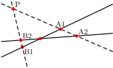
First of all, one can safely assume that l1 and l2 are different. If not, then the identity function works just fine. The first step of the proof is to write a function which, given two lines l1 and l2 computes a point P which belongs neither to l1 nor to l2.
Lemma outsider : forall l1 l2: Line,
{P:Point | ~Incid P l1/\~Incid P l2}.
A1 P b bA2 b B2 b B1 b b
D
PG(2,5)
P30P29P28P27P26P25P24P23P22P21P20P19P18P17P16P15P14P13P12P11P10P9P8 P7P6P5P4 P3 P2P1P0 1 2 3 4 5 6 7 8 9 10 11 12 13 14 15 16 17 18 19 20 21 22 23 24 25 26 27 28 29 30 0 2 3 4 5 6 7 8 9 10 11 12 13 14 15 16 17 18 19 20 21 22 23 24 25 26 27 28 29 30 0 1 4 5 6 7 8 9 10 11 12 13 14 15 16 17 18 19 20 21 22 23 24 25 26 27 28 29 30 0 1 2 3 9 10 11 12 13 14 15 16 17 18 19 20 21 22 23 24 25 26 27 28 29 30 0 1 2 3 4 5 6 7 8 13 14 15 16 17 18 19 20 21 22 23 24 25 26 27 28 29 30 0 1 2 3 4 5 6 7 8 9 10 11 12 19 20 21 22 23 24 25 26 27 28 29 30 0 1 2 3 4 5 6 7 8 9 10 11 12 13 14 15 16 17 18We now explicitly construct the function f as shown on Figure 5. Given a point A1 of l1, we can build a line (say ∆) going through A1 and P . Lines ∆ and l2intersect in a point A2. We define f such that f (A1) = A2. It remains to prove that this function is actually bijective. Proving that this function is one-to-one requires to assume proof irrelevance [22]. Proof irrelevance expresses that proofs of the same formula are equal. It allows us to show existential propositions with the same type are equal regardless of the proof terms proving the formulas. Proving the onto property requires to apply the construction process of f in the reverse order going from line l2 to line l1.
References
[1] Yves Bertot and Pierre Castéran. Interactive Theorem Proving and Program
De-velopment, Coq’Art: The Calculus of Inductive Constructions. Texts in
Theoreti-cal Computer Science. An EATCS Series. Springer, 2004.
[2] Marc Bezem and Dimitri Hendriks. On the Mechanization of the Proof of Hessen-berg’s Theorem in Coherent Logic. Journal of Automated Reasoning, 40(1):61–85, 2008.
[3] Francis Buekenhout, editor. Handbook of Incidence Geometry. North Holland, 1995.
[4] Cinzia Cerroni. Non-Desarguian Geometries and the Foundations of Geometry from David Hilbert to Ruth Moufang. Historia Mathematica, 31(3):320–336, 2004. [5] Shang-Ching Chou, Xiao-Shan Gao, and Jing-Zhong Zhang. Machine Proofs in
Geometry. Series on Applied Mathematics. World Scientific, 1994.
[6] Jacek Chrzaszcz. Implementing Modules in the Coq System. In Theorem Proving
in Higher-Order Logics, volume 2758 of LNCS, pages 270–286. Springer-Verlag,
2003.
[7] Coq development team, The. The Coq Proof Assistant Reference Manual, Version
8.0. LogiCal Project, 2004.
[8] Harold Scott Macdonald Coxeter. Projective Geometry. Springer, 1987.
[9] Jérôme Créci and Loïc Pottier. Gb: une procédure de décision pour Coq. In Actes
JFLA 2004, 2004. In french.
[10] Christophe Dehlinger, Jean-François Dufourd, and Pascal Schreck. Higher-Order Intuitionistic Formalization and Proofs in Hilbert’s Elementary Geometry. In
Automated Deduction in Geometry 2000, volume 2061 of LNCS, pages 306–324.
Springer-Verlag, 2000.
[11] Jean Duprat. Une axiomatique de la géométrie plane en Coq. In Actes des JFLA
2008, pages 123–136. INRIA, 2008. In french.
[12] Jean Duprat, Frédérique Guilhot, and Julien Narboux. Toward a “common” lan-guage for formally stating elementary geometry theorems, 2008. Draft.
[13] Frédérique Guilhot. Formalisation en Coq et visualisation d’un cours de géométrie pour le lycée. Revue des Sciences et Technologies de l’Information, Technique et
Science Informatiques, Langages applicatifs, 24:1113–1138, 2005. In french.
[14] Arend Heyting. Axioms for intuitionistic plane affine geometry. In P. Suppes L. Henkin and A. Tarski, editors, The axiomatic Method, with special reference to
Geometry and Physics, pages 160–173, Amsterdam, 1959. North-Holland.
[15] Christoph M. Hoffmann and Robert Joan-Arinyo. Handbook of Computer Aided
[16] Christophe Jermann, Gilles Trombettoni, Bertrand Neveu, and Pascal Mathis. Decomposition of Geometric Constraint Systems: a Survey. International Journal
of Computational Geometry and Application, 16(5-6):379–414, november 2006.
[17] Hongbo Li and Yihong Wu. Automated Short Proof Generation for Projective Geometric Theorems with Cayley and Bracket Algebras: I. incidence geometry.
J. Symb. Comput., 36(5):717–762, 2003.
[18] Nicolas Magaud, Julien Narboux, and Pascal Schreck. Formalizing Desargues’ theorem in Coq using ranks. In Proceedings of the ACM Symposium on Applied
Computing SAC 2009. ACM, ACM Press, March 2009.
[19] Laura Meikle and Jacques Fleuriot. Formalizing Hilbert’s Grundlagen in Is-abelle/Isar. In Theorem Proving in Higher Order Logics, volume 2758 of LNCS, pages 319–334. Springer, 2003.
[20] Laura Meikle and Jacques Fleuriot. Mechanical Theorem Proving in Computa-tional Geometry. In Hoon Hong and Dongming Wang, editors, Automated
De-duction in Geometry 2004, volume 3763 of LNCS, pages 1–18. Springer-Verlag,
November 2005.
[21] Dominique Michelucci, Sebti Foufou, Loïc Lamarque, and Pascal Schreck. Ge-ometric constraints solving: some tracks. In SPM ’06: Proceedings of the 2006
ACM symposium on Solid and physical modeling, pages 185–196. ACM, ACM
Press, New York, USA, 2006.
[22] Alexandre Miquel and Benjamin Werner. The Not So Simple Proof-Irrelevant Model of CC. In Herman Geuvers and Freek Wiedijk, editors, TYPES 2002, volume 2646 of LNCS, pages 240–258. Springer, 2002.
[23] Forest Ray Moulton. A Simple Non-Desarguesian Plane Geometry. Transactions
of the American Mathematical Society, (3):192–195, 1902.
[24] Julien Narboux. A Decision Procedure for Geometry in Coq. In Slind Konrad, Bunker Annett, and Gopalakrishnan Ganesh, editors, TPHOLs’2004, volume 3223 of LNCS. Springer-Verlag, 2004.
[25] Julien Narboux. Mechanical Theorem Proving in Tarski’s Geometry. In
Post-proceedings of Automatic Deduction in Geometry 06, volume 4869 of LNAI, pages
139–156. Springer-Verlag, 2007.
[26] Lawrence C. Paulson. The Isabelle reference manual, 2006.
[27] David Pichardie and Yves Bertot. Formalizing Convex Hulls Algorithms. In Proc.
of 14th International Conference on Theorem Proving in Higher Order Logics (TPHOLs’01), volume 2152 of LNCS, pages 346–361. Springer-Verlag, 2001.
[28] Jürgen Richter-Gebert. Mechanical Theorem Proving in Projective Geometry.
Ann. Math. Artif. Intell., 13(1-2):139–172, 1995.
[29] Pascal Schreck. Robustness in CAD Geometric Construction. In 5th International
Conference on Information Visualisation IV2001, pages 111–116, London, july
2001.
[30] Wolfram Schwabhauser, Wanda Szmielew, and Alfred Tarski. Metamathematische
Methoden in der Geometrie. Springer-Verlag, 1983. In german.
[31] Carlos Simpson. Computer Theorem Proving in Math, April 2004. http://hal.archives-ouvertes.fr/hal-00000842/en/.
[32] Matthieu Sozeau and Nicolas Oury. First-Class Type Classes. In Proceedings of
TPHOLs 08, volume 5170 of LNCS, pages 278–293. Springer, 2008.
[33] Alfred Tarski. What is Elementary Geometry? In L. Henkin, P. Suppes, and A. Tarski, editors, The axiomatic Method, with special reference to Geometry and
Physics, pages 16–29, Amsterdam, 1959. North-Holland.
[34] Jan von Plato. The Axioms of Constructive Geometry. In Annals of Pure and