HAL Id: hal-02998908
https://hal.archives-ouvertes.fr/hal-02998908
Submitted on 24 Nov 2020
HAL is a multi-disciplinary open access
archive for the deposit and dissemination of
sci-entific research documents, whether they are
pub-lished or not. The documents may come from
teaching and research institutions in France or
abroad, or from public or private research centers.
L’archive ouverte pluridisciplinaire HAL, est
destinée au dépôt et à la diffusion de documents
scientifiques de niveau recherche, publiés ou non,
émanant des établissements d’enseignement et de
recherche français ou étrangers, des laboratoires
publics ou privés.
Magnetic cusp confinement in low-β plasmas revisited
Yuchao Jiang, G. Fubiani, Laurent Garrigues, J. Boeuf
To cite this version:
Yuchao Jiang, G. Fubiani, Laurent Garrigues, J. Boeuf.
Magnetic cusp confinement in low-β
plasmas revisited. Physics of Plasmas, American Institute of Physics, 2020, 27 (11), pp.113506.
�10.1063/5.0014058�. �hal-02998908�
1
Magnetic cusp confinement in low- plasmas revisited
Y. Jiang, G. Fubiani, L. Garrigues, J.P. Boeuf
aLAPLACE, Université de Toulouse, CNRS, INPT, UPS, 118 Route de Narbonne, 31062 Toulouse, France
ABSTRACT
Magnetic cusps have been used for more than 50 years to limit charged particle losses to the walls and confine the plasma in a large variety of plasma sources or ion sources. Quantification of the effective loss area has been the subject of many experimental as well as theoretical investigations in the 1970-1990’s. In spite of these efforts there is no fully reliable expression of the effective wall loss as a function of cusp magnetic field, electron temperature, ion mass, gas pressure, etc… We describe in this paper a first attempt at obtaining scaling laws for the effective loss width of magnetic cusps, based on two-dimensional PIC MCC (Particle-In-Cell Monte Carlo Collisions) simulations. The results show that the calculated leak width follows a 1/B scaling in the collisionless low B limit, is approximately proportional to the hybrid gyroradius with an ion velocity equal to the Bohm velocity and is proportional to the square root of gas pressure in the collisional limit.
I. INTRODUCTION
Plasma confinement by magnetic cusps has been studied since the 1970’s when Limpaecher and MacKenzie1 showed
that they could increase the plasma density in a low pressure discharge by two orders of magnitude by employing multipolar cusp confinement. A number of experimental as well as theoretical papers were published in the 1970-1980’s on magnetic cusps. They were initially studied as possible confinement methods for thermonuclear fusion2, 3, but they
were actually more used for basic plasma studies. Magnetic cusps are now commonly used in different types of ion sources or in plasma processing reactors, but, in spite of the important efforts to quantify the role of magnetic cusps on plasma confinement, there is still no clear scaling laws that give the effective charged particle loss area or loss width in the presence of cusps, as a function of plasma parameters such as electron temperature, gas pressure, magnetic field and ion mass. In their 1975 paper, Hershkowitz et al.4 mention
(and this is still true today) that “Although the motion of charged particles in magnetic cusps has received considerable attention, a satisfactory description of how plasma leaks through cusps has not yet emerged. In particular, there seems to be considerable disagreement between theory and experiments”.
Semi-empirical theories have been proposed to quantify the effective loss area and their predictions have been compared with numerous experimental results but the agreement between theory and experiments was only qualitative and in a limited parameter range. The availability of powerful simulation tools and computers should allow us to progress toward a more quantitative description of the confinement by magnetic cusps. This paper presents an attempt at obtaining
a Electronic mail: [email protected]
scaling laws for the effective loss width of magnetic cusps, based on 2D PIC MCC simulations.
One difficulty in trying to extract scaling laws from the experiments is that the results may depend on the type of plasma source and on the magnetic cusp arrangement. In most early experiments the plasma was generated by hot filaments. In the experiments of Limpaecher and MacKenzie1 the
magnetic cusps were produced by lining the inner wall of the vacuum chamber with permanent magnets1 while in those of
Hershkowitz et al.4-6 they were formed by a “picket fence”,
i.e. an arrangement of parallel water-cooled conductors with current in adjacent conductors flowing in alternate directions. The picket fence was placed between two single multidipole chambers, the “driver chamber” (where the plasma was generated by hot filaments) and the “target chamber”. In practical applications, multicusp plasma sources are used in plasma processing or in ion sources, e.g. for satellite propulsion7-9 or negative ion sources for accelerators10
(including neutral beam injectors for fusion). In these sources the plasma can be generated by filaments or by radiofrequency or microwave coupling. The multicusp magnets are generally placed behind metallic chamber walls but in some devices11 they are covered with a dielectric
material. Clearly the electron velocity distribution functions and the localization of ionization with respect to the magnetic cusps can be very different in the different multicusp plasma source configurations used in the applications. In this paper we choose to model, using a 2D PIC MCC simulation, an ideal situation where the electron distribution function is Maxwellian with a fixed temperature, where the ionization source is sufficiently far from the cusp region, and with multicusp magnets covered with a dielectric material. The model is purely kinetic and is able to describe quasi-neutral
2 regions as well as sheaths. Although electron-neutral and ion-neutral mean free paths are larger than the dimensions of the simulation domain in most of the conditions considered here, the results show that electron-neutral collisions significantly contribute to cross-field diffusion leading to an increase of the leak width with gas pressure above 0.1 mtorr. Electrons reflected by the cusp or the sheath back into the plasma are supposed to be thermalized. This procedure prevents trapping of low energy electrons and can represent, for example, the effect of Coulomb collisions.
The paper is organized as follows.
Section II presents a brief overview of previous experimental and theoretical work on magnetic cusps. Details about the assumptions of the 2D PIC MCC model of magnetic cusps used in this paper are given in section III. In section IV we show typical results concerning the general properties of the plasma in the cusps regions (distribution of charged particle densities, electric potential, charged particle fluxes etc…). Section V summarizes the scaling laws deduced from a parameter study of the leak width as a function of different parameters such as magnetic field, gas pressure, electron and ion temperatures, ion mass. In section VI we briefly discuss the question of convergence and accuracy of the simulation.
II. BRIEF OVERVIEW OF PREVIOUS WORKS
We summarize below the experimental and modeling efforts that have been devoted to the characterization of cusp confinement. We are considering here only low- plasmas, i.e. plasmas where the plasma pressure is much less than the magnetic pressure. In these plasmas the external magnetic field is not modified by the charged particles currents. In the following, we note 𝑤∗, the leak width defined as the Full
Width at Half Maximum (FWHM) of the profile of the current density to the wall (see Figure 1). This definition of the leak width is used in experiments but we will use a slightly different definition in the simulations (see section III.G). For a metallic surface the electron and ion current density profiles are not necessarily identical, and one could define specific leak widths for electrons and ions. As shown in the experiments of Bosch and Merlino12, the electron and ion leak
widths should however become close to each other when the plasma density increases (because the plasma becomes quasineutral in a larger volume and close to the surface). For a dielectric surface one expects the electron and ion loss widths to be identical at steady state.
Most theories for high- plasmas2-4 predicted a loss aperture
or leak width 𝑤∗ between the electron gyroradius 𝜌
𝑒 and the
hybrid gyroradius defined as (𝜌𝑒𝜌𝑖)1/2 (geometric mean of
the electron and ion gyroradii ρe and ρi) while experiments
found different results lying between the ion gyroradius, the hybrid gyroradius and the electron gyroradius.
Figure 1: Schematic of a line magnetic cusp. To the first order in
Δ 𝑑⁄ the magnetic field decreases exponentially from the wall
surface to the plasma. The red line is the charged particle current
density J to the wall. The leak width 𝑤∗ is defined in experiments
as the Full Width at Half maximum of the current density profile.
In the model of Bosch and Merlino12 (see text) ions flow toward
the cusp along the magnetic field lines at the ion acoustic velocity; collisional cross-field diffusion of electrons tends to spread the current density in the cusp and increases the leak width.
The first measurements of the leak width in low- plasmas where performed in 1975 by Hershowitz et al. 4. They found
that the electron leak width (FWHM) at low enough gas pressures was about four times the hybrid gyroradius: 𝑤𝐻∗ ≈ 4(𝜌𝑒𝜌𝑖)1/2 (1)
The measured ion leak width was slightly larger than the electron leak width. As said in the introduction, the measurements were performed in a plasma source divided in two regions, the driver and the target, separated by a “picket fence” structure consisting of an array of parallel conductor wires with currents in adjacent conductors flowing in alternating directions. The plasma was sustained by high energy electrons emitted from hot filaments in the driver. The leak width was deduced from measurements of the electron and ion current through the picket fence (i.e. between the wires of the picket fence). The measurements were performed in helium, argon, and xenon, and confirmed the 𝑚𝑖1/4
dependence of the leak width present in the expression of the hybrid gyroradius (𝑚𝑖 is the ion mass). The 1/𝐵 dependence
of this expression was also checked (over a limited range of values of the magnetic field, between 50 and 200 G). We write the electron and ion gyroradii as:
𝜌𝛼= 𝑣𝛼⁄𝜔𝑐𝛼 , 𝛼 = 𝑒, 𝑖, where 𝑣𝛼= (𝑘𝑇𝛼⁄𝑒𝑚𝛼)1/2 is the
charged particle velocity, and 𝜔𝑐𝛼 = 𝑒𝐵 𝑚⁄ 𝛼 is the
corresponding cyclotron frequency. Since 𝜌𝑖
𝜌𝑒= ( 𝑇𝑖 𝑇𝑒 𝑚𝑖 𝑚𝑒) 1/2 , the leak width of Herskowitz et al. can also be written as: 𝑤𝐻∗ ≈ 4𝜌𝑒( 𝑇𝑖 𝑇𝑒 𝑚𝑖 𝑚𝑒) 1/4 ∝ 𝑇𝑒1/4𝑇𝑖1/4𝑚𝑖1/4𝐵−1 (2)
Note that the ion gyroradius in the experiments of Hershkowitz et al. is on the order of 3.5 cm for argon, and 5.6 cm in xenon for a magnetic field of 100 G (see Table I in Ref.
4). Since the distance between wires (or cusps) was 2.2 cm in
this paper, it appears that ions are practically not magnetized in these experiments. Therefore the fact that the ion
3 gyroradius appears in eq. (1) seems purely fortuitous and does not have a real physical meaning. We see below that Bosch and Merlino12 obtained a similar scaling based on an
empirical theory that does not invoke the ion gyroradius. Bosch and Merlino12 performed similar experiments in ring
and point cusps over magnetic field strengths between 10 and 260 G and neutral gas pressures between 10-2 and 10 mtorr.
The magnetic field was generated by two water-cooled coils of 17 cm inner diameter that produced a spindle cusp and a ring cusp magnetic field using currents of up to 1000 A. The maximum magnetic field in the center of the ring cusp was 160 G, while the maximum field in the center of the point cusp was 260 G. The measured current profiles presented a sharp maximum in the cusp center. The ion leak width was larger than the electron leak width, but the current profiles became closer together when the plasma density was increased. The measurements of Bosch and Merlino showed that the variations of the leak widths with gas pressure was close to 𝑝1/2 and that the leak widths varied as 𝐵−1 at
relatively low magnetic field, and as 𝐵−1/2 at higher
magnetic fields. The breakdown of the 𝐵−1 dependence of the
leak width at high magnetic field and low pressure was attributed to the fact that collisional, ∝ 𝐵−2 diffusion was
replaced by anomalous or Bohm, ∝ 𝐵−1 diffusion at higher
magnetic field. Considering ambipolar diffusion across the magnetic field and assuming that the plasma in the cusps is flowing outward at approximately the ion acoustic speed, Bosch and Merlino12 derived the following approximate
expression of the ring cusp leak width: 𝑤𝐵𝑀∗ ≈ (2𝐷̅𝑅 𝐶⁄ )𝑠 1/2
where 𝐷̅ is the electron cross-field diffusion coefficient, and 𝐶𝑠 is the ion Bohm velocity. 𝑅 was the radius of the ring cusp.
We generalize this expression to a picket fence or a multicusp geometry with a distance 𝑑 between cusps, by taking 𝑑 ≈ 2𝑅 and the leak width becomes:
𝑤𝐵𝑀∗ ≈ (𝑑𝐷̅ 𝐶⁄ )𝑠 1/2
This expression is derived semi-empirically but it is interesting to look at the scaling of this expression with the different plasma parameters.
The collisional diffusion coefficient 𝐷̅ can be written as: 𝐷̅ = 𝑘𝑇𝑒 𝑒 𝑒 𝑚𝑒 𝜈𝑒𝑁 𝜔𝑐𝑒2
where 𝜈𝑒𝑁 is the electron-neutral collision frequency (the
electron-ion Coulomb collision frequency should be added at high plasma densities). Introducing the electron mean free path 𝜆𝑒𝑁 = 𝑣𝑒⁄𝜈𝑒𝑁, we get: 𝑤𝐵𝑀∗ ≈ ( 𝑑 𝜆𝑒𝑁) 1/2 𝜌𝑒( 𝑚𝑖 𝑚𝑒) 1/4 (3) The scaling of the leak width in that case is:
𝑤𝐵𝑀∗ ∝ 𝜆𝑒𝑁−1/2𝑇𝑒1/2𝑚𝑖1/4𝐵−1
The expression of Bosch and Merlino of eq. (3) can also be written 𝑤𝐵𝑀∗ ≈ ( 𝑑 𝜆𝑒𝑁) 1/2 (𝜌𝑒𝜌𝑖,𝐵𝑜ℎ𝑚) 1/2 i.e. is proportional to
the hybrid gyroradius as in the expression of Hershkowitz et al. but if the hybrid radius in 𝑤𝐻∗ is calculated for an ion
velocity equal to the Bohm velocity and if the electron mean free path 𝜆𝑒𝑁 does not depend on electron temperature (which
is generally not the case). If the electron mean free path 𝜆𝑒𝑁
is constant, the leak width scales as 𝑇𝑒1/2 but if the electron
collision frequency 𝜈𝑒𝑁 is constant, the leak width scales as
𝑇𝑒1/4. In argon, because of the Ramsauer minimum, the
electron cross-section increases significantly between 0.1 and 10 eV so the mean free path decreases with electron temperature. According to the expression above, the leak width 𝑤𝐵𝑀∗ should therefore increase faster than 𝑇𝑒1/2.
The advantage of the Bosch and Merlino’s expression of the leak width is that it takes into account the gas pressure and distance between cusps. It is clear that the leak width should increase with gas pressure due to the increased collisional diffusion of electrons across the magnetic field. Since the electron mean free path is inversely proportional to the gas density or to the gas pressure 𝑝, the leak width of Bosch and Merlino scales as 𝑝1/2. Numerically, if the magnetic field in
the electron and ion Larmor radii is taken as the maximum magnetic field (i.e. 𝐵0) in the expression of the leak width,
the value of 𝑤𝐵𝑀∗ can be actually much smaller than the
measured one. For example, at 0.1 mtorr, the electron mean free path is several meters, much larger than 𝑑 (17 cm) in the experiment of Bosch and Merlino so that 𝑤𝐵𝑀∗ =
( 𝑑
𝜆𝑒𝑁) 1/2
𝑤𝐻∗ ≪ 𝑤𝐻∗. Bosch and Merlino12 and other authors11, 13, 14 argue that in the expression of 𝑤
𝐵𝑀∗ , the diffusion
coefficient (or the Larmor radii) should not be estimated at the point of maximum magnetic field. Bosch and Merlino estimate the diffusion coefficient at a point midway between the cusp and the filament. Cooper et al.11 mention that the
Bosch and Merlino model uses “ill-defined fitting parameters 𝐵 and 𝑑 which can always be selected to fit the data over a small scaling”. These authors developed a 1D numerical model based on the 0D model of Bosch and Merlino (i.e., with perpendicular cross-field diffusion and outward plasma flow through the cusp at the Bohm velocity). This allows to get a more self-consistent dependence of the leak width on the magnetic field. They find a good scaling with their experiment on the WiPAL multicusp plasma source11.
Unfortunately, this paper does not show the measured variations of the leak width as a function of the different parameters (magnetic field, electron temperature, pressure …) that could be very useful for model comparisons. In recent experiments Hubble et al.15 were able to measure 2D
electron density profiles around magnetic cusps using an original, non-intrusive diagnostic technique (Laser-Collision Induced Fluorescence). They deduce from these measurements that the leak width scaled as the hybrid gyroradius, with a scaling constant of proportionality increasing with pressure.
Finally, a third expression of the leak width was derived by Koch and Mathieussent16:
4 𝑤𝐾𝑀∗ = 2𝑑 𝜋 ( 𝜌𝑒𝜌𝑖 𝜆𝑒𝜆𝑖) 1/2 (4) The scaling of this expression with ion mass and magnetic field is 𝑚𝑖1/4𝐵−1, i.e. is identical to that of Herskowitz et al.
and Bosch and Merlino. However the leak width of Koch and Mathieussent is proportional to the gas pressure 𝑝 instead of 𝑝1/2 in the expression of Bosch and Merlino. Note also that
this leak width is proportional to the distance 𝑑 between cusps while the expression of Bosch and Merlino varies as 𝑑1/2.
Bosch and Gilgenbach17 give a simple and interesting
discussion of the scaling laws deduced from the different models. For example, they show that the expression 𝑤𝐾𝑀∗ of
Koch and Mathieussent can be considered as the continuation of that of Bosh and Merlino, 𝑤𝐵𝑀∗ , when the pressure is large
enough so that particle losses parallel to the magnetic field, in the cusps, can no longer be described by ions at the Bohm velocity, but must be represented by parallel ambipolar diffusion. In that case the expression of Bosch and Merlino can be re-written by replacing 𝐶𝑠 by 𝐷∥⁄ , with 𝐷𝑑 ∥=
𝑘𝑇𝑒⁄(𝑚𝑖𝜈𝑖𝑁) where 𝜈𝑖𝑁 is the ion-neutral collision frequency
and 𝑤𝐵𝑀∗ becomes: 𝑤𝐵𝑀∗ ≈ (𝑑𝐷̅ 𝐶⁄ )𝑠 1 2→ 𝑤𝐾𝑀∗ ≈ 𝑑 (𝑚𝑖 𝑚𝑒 𝜈𝑒𝑁𝜈𝑖𝑁 𝜔𝑐𝑒2 ) 1/2 = 𝑑 (𝜌𝑒𝜌𝑖 𝜆𝑒𝜆𝑖) 1/2
where we have used 𝜆𝑒𝑁 = 𝑣𝑒⁄𝜈𝑒𝑁 and 𝜆𝑖𝑁 = 𝑣𝑖⁄𝜈𝑒𝑁 .
This expression is similar to that of Koch and Mathieussent. Again, the coefficients in front of these expressions are not accurate since these derivations are very approximative and only the scaling with the different parameters should be considered. The above derivation of Bosch and Gilgenbach provides a good justification of the (𝑑𝑝)1/2 scaling of the leak
width of Bosch and Merlino, in comparison with the 𝑑𝑝 scaling of Koch and Mathieussent. Note also that, for consistency, if the expression of Koch and Mathieussent is used, the velocity in the ion Larmor radius should be the ion thermal velocity and not the Bohm velocity. Therefore, the scaling of 𝑤𝐾𝑀∗ 𝑤ith temperatures is as (𝑇𝑒𝑇𝑖)1/4 instead of
𝑇𝑒1/2 for 𝑤𝐵𝑀∗ .
It is interesting to look at the ranges of pressure where the leak width 𝑤𝐵𝑀∗ or 𝑤𝐾𝑀∗ should be used, for example in argon.
The charge exchange cross-section 𝜎 of argon ions is on the order of 4x10-19 m2. Therefore, for a pressure of 1 mtorr (gas
density 𝑁𝑔 on the order of 3.5x10¹⁹ m-3), the ion mean free
path 𝜆𝑖𝑁= 1 (𝑁⁄ 𝑔𝜎) is about 7 cm. If the distance between
magnets is on the order of 1 to 2 cm, the expression 𝑤𝐿,𝐵𝑀 of
Bosch and Merlino should provide a good scaling up to several mtorr, while the expression 𝑤𝐾𝑀∗ of Koch and
Mathieussent would be probably better above 10 mtorr (i.e. for pressures where cusp confinement is actually not efficient).
Apart from these semi-empirical analytical determinations of the leak width of magnetic cusps, we can mention the particle simulations of Marcus et al.18 and of Takekida and Nanbu19.
Marcus et al. .18 performed a 2D PIC simulation of a periodic
“picket fence” for Maxwellian electron and ion velocity
distribution functions and a collisionless plasma. The assumptions of this model were very similar to those of the resent paper (periodicity, Maxwellian distribution functions, method of generation of the plasma, see section III below). Due to limitations on the computing power available at that time, they used unrealistic mass ratios 𝑚𝑖⁄𝑚𝑒 (between 64
and 256) and did not perform systematic parameter studies of the leak width. Nevertheless, they were able to confirm that, in their collisionless conditions, the ion leak width was on the order of the hybrid gyroradius and that the electron leak width was about twice smaller than the ion leak width (this however should depend on the plasma density, as shown by Bosch and Merlino12).
The assumptions of the particle model of Takekida and Nanbu19 were different from those of Marcus et al.. The
plasma was generated by a hot plasma filament placed in the center of a 2D cylindrical multicusp grounded plasma reactor. The computation domain included a section between two successive magnetic cusps of the circular cross-section of the reactor, assuming periodic boundary conditions. In this configuration of plasma generated by hot filament at a negative potential with respect to the chamber walls, there is a net current between the filament and the chamber walls. This is different from the conditions of the paper of Marcus et al. where the total electron and ion fluxes through the picket fence must be equal, or from the configuration of the present paper where the chamber walls are covered with a dielectric layer. Takekida and Nanbu used this model to study the variations of the plasma density and the potential distribution with magnetic field, number of magnets and pressure but did not provide information about the effective leak width of the chamber as a function of these parameters.
III. PIC MCC MODEL OF A MULTICUSP PLASMA
SOURCE
A. Simulation domain
We consider a 2D rectangular geometry with line cusps infinite in the direction perpendicular to the simulation domain and periodic in the direction parallel to the walls, as shown in Figure 2.
The walls are made of dielectric materials, i.e. the electron and ion fluxes to the wall must be identical at steady state. The dimensions of the domain in the simulations presented here are 𝐿𝑥= 4 cm and 𝐿𝑦= 2 cm . The distance between
cusps is 𝑑 = 1 cm . The magnetic field intensity (top) decreases exponentially from the walls. Electrons are thermalized (see section III.E) inside the region indicated by the dashed lines.
5
Figure 2: Simulation domain for the 2D PIC MCC simulation of magnetic cusps. The axial distribution of the magnetic field intensity is shown on top of the simulation domain
Because of the symmetries of the problem, the simulation domain can be divided in two in each direction. Most simulations have been performed in the grey domain of Figure 2, with symmetry boundary conditions on the right boundary, periodic boundary conditions for the potential and charged particle reflection on the top and bottom boundaries (we checked that these boundary conditions lead to the same results than the simulation of the whole domain). This can significantly speed up the simulations. The boundary condition for the wall potential in Poisson’s equation is obtained from the calculated surface charge (see sections III.C and III.E).
B. Magnetic field distribution
We use an analytical expression of the magnetic field derived by Lieberman and Lichtenberg20 based on a first order
development in the assumed small parameter Δ 𝑑⁄ where Δ is the width of the magnets and 𝑑 their distance (see Figure 2). In this approximation, the x and y components of the magnetic field due to the magnets on the left side of the simulation domain can be written as:
𝐵𝑥= 𝐵0sin ( 𝜋𝑦 𝑑) 𝑒 −𝜋𝑥 𝑑 𝐵𝑦= −𝐵0cos (𝜋𝑦 𝑑) 𝑒 −𝜋𝑥 𝑑
Figure 3: Distribution of the magnetic field (color scale) and
magnetic field lines (black lines) used in the simulations. B0 is
the magnetic field intensity on the dielectric wall.
Note that the magnetic field intensity 𝐵 = √𝐵𝑥2+ 𝐵𝑦 2
= 𝐵0𝑒−
𝜋𝑥
𝑑 does not depend on 𝑦. The magnet width Δ does not
affect the magnetic field distribution but only the value of 𝐵0.
Since we assume low 𝛽 plasma conditions, the magnetic field is not modified by the plasma and is not re-calculated during the simulation. This is justified since the electron pressure 𝑝𝑒= 𝑒𝑛𝑒T𝑒 (the electron temperature T𝑒 is expressed in eV)
in our conditions is typically less than 2x10⁻³ Pa (plasma
density of a few 1015 m-3 and electron temperature of a few
eV) while the magnetic pressure 𝑝𝐵= 𝐵2⁄2𝜇0 is on the order
of 5x10⁻³𝐵
𝐺𝑎𝑢𝑠𝑠2 . Therefore 𝛽 = 𝑝𝑒⁄𝑝𝐵 is much smaller than
1 in our conditions, even for magnetic fields where the magnetization of electrons is negligible. For larger plasma densities, typical of low temperature plasma sources, i.e. on the order of 1018 m-3, 𝛽 becomes closer to 1 for magnetic
fields of about 5 G, i.e. at the entrance of the cusp region. The study of possible consequences of larger values of 𝛽 in this region is outside the scope of this paper.
C. Particle-In-Cell Monte Carlo Collision model
The particle simulation code used in this paper is the same as the one described in previous publications21-25. It is an
explicit electrostatic 2D Particle-In-Cell Monte Carlo Collisions code. The code is parallelized in the Open MP framework and has been run on multi-core processors with up to 12 cores. The results of the simulations have been cross-checked with those obtained from two other similar codes developed separately26, 27 and using a hybrid Open MP + MPI
parallelization method. The agreement between the different codes was better than 5 % for the leak width over the range of parameters considered in this paper. The parallelization of these codes is based on particles (i.e. similar number of particles are treated in parallel on each core).
The model uses a classical leap-frog Buneman-Boris algorithm28 for the time integration of the charged particles
trajectories. Time integration is explicit, i.e. the electric field is calculated from Poisson’s equation at the beginning of each time step and is supposed to be constant when the particles are moved over one time step. Charged particle reaching the dielectric wall are not reflected. The surface charge is calculated by integrating the current densities to the dielectric wall and the potential boundary conditions on the wall is calculated as described in section III.E. Explicit simulations imply constraints on the time step and grid spacing28, 29. We
used a 192x96 nodes grid over the 2 cm x 1 cm simulation domain in the simulations presented here. The grid spacing 𝛿𝑥 (≈ 100 μm) and integration time step 𝛿𝑡 (= 5x10-11 s)
were such that 𝛿𝑥 𝜆⁄ 𝐷 ≈ 0.7 and 𝜔𝑝𝛿𝑡 ≈ 0.2 where 𝜆𝐷 and
𝜔𝑝 are respectively the electron Debye length and plasma
frequency. For large values of the magnetic field (on the order of 0.1 T), the time step was therefore such that 𝜔𝑐𝛿𝑡 ≈ 1
where 𝜔𝑐 is the maximum electron cyclotron frequency. This
corresponds to about 6 integration time steps over one electron gyroradius (the cyclotron period is 2𝜋 𝜔⁄ 𝑐). We
6 checked that decreasing the time step by a factor of 2 did not change significantly the collected current and leak width. We also performed simulations with larger number of grid points (256x128 and 512x256). The maximum differences in the calculated potential distribution was less the 0.5 V, and the change in the collected current was not significant. The average number of charged particles per cell was about 50 in the results presented below. We checked the convergence of the results with the number of particles per cell. The results of these tests are shown in section VI.
The Monte Carlo Collisions module is implemented as described in Ref. 29. Electron and ion collisions with atoms in
the ground state are considered (atoms are supposed to be at ambient temperature and the atom velocity is neglected with respect to the electron and ion velocities in the collision process). The collision cross-sections and others parameters are described in section III. D below.
D. Collisions cross-sections and characteristic length and time scales.
The electron-argon cross-section are taken from the simplified set of A.V. Phelps in the LXcat database30 plotted
in Figure 4. In this cross-section set the electronic excitation cross-sections are grouped in one single cross-section of threshold 11.5 eV. Therefore, three electron cross-sections are considered, momentum exchange, excitation and ionization (ionization is treated as an excitation, see III.F)). In this paper we consider gas pressures from 0.01 mtorr to a few mtorrs. The gas density 𝑁𝑔 at 1 mtorr is about 3.5x10¹⁹
m-3 and the electron-neutral momentum cross-section of a 3
eV electron is on the order of 𝜎 ≈ 2x10-20 m2 (Figure 4). The
mean free path 𝜆𝑒𝑁= 1 𝑁⁄ 𝑔𝜎 of a 3 eV electron therefore
varies from 150 m at 0.01 mtorr, to 0.5 m at 3 mtorr, while the electron-neutral collision frequency 𝜈 = 𝑁𝑔𝜎𝑣 varies
approximately from 3x10⁴ s-1 to 107 s-1 in the same pressure
range. Note that because of the Ramsauer minimum in argon, the electron-neutral momentum cross-section increases by a factor of 10 between 1 eV and 10 eV, so the momentum collision frequency also increases by a factor of 10 while the electron mean free path decreases by a factor of 10 in this energy range.
Figure 4: Simplified set of electron-argon cross-section (from the
Phelps data base in LXcat 30).
The ion-neutral charge exchange cross-section is taken as a constant in the smulations, equal to 4x10-19 m2. The ion mean
free path for charge exchange collisions therefore varies from 10 m at 0.01 mtorr, to 3 cm at 3 mtorr. These dimensions are larger than the dimensions of our simulation domain. Since the ions are practically not magnetized in our conditions, and are not trapped by the magnetic field, we can consider that the ion-neutral collisions do not play an essential role in our pressure range.
For electron and ion temperatures of 2 eV and 0.5 eV respectively, which are typical of the simulations below, the electron and ion gyroradii, 𝜌𝑒 and 𝜌𝑖, in argon and for a
magnetic field of 100 G are respectively on the order of 0.25 mm and 5 cm (and are smaller for larger magnetic fields). Since the cusp length 𝑑 is 1 cm in our simulations, we can say than the ions are not magnetized for 𝐵 = 100 G. For the largest magnetic fields used in the simulation, on the order of 𝐵 = 1000 G, the minimum ion gyroradius is about 5 mm. Since the leak width in that case is smaller than the ion gyroradius we can still consider that ions are not or are only weakly magnetized.
The electron Debye length 𝜆𝐷 in the simulations is about 0.1
mm, is close to the electron gyroradius for low magnetic fields and about 4 times larger than 𝜌𝑒 for 𝐵 = 1000 G.
Finally, note that because electrons returning to the plasma center (electron thermalization region of Figure 2) are thermalized at a relatively high frequency (i.e. their velocity is modified according to an isotropic Maxwellian distribution at 𝑇𝑒), electrons cannot be trapped in the simulation, even if
their velocity is not in the loss cone. The thermalizing frequency was 109 s-1 in the simulations. Since the transit time
of a 2 ev electron from the cusp to the plasma is on the order of 10-8 s, most electrons outside the loss cone are reflected
only once before their velocity is changed. We performed simulations with a lower thermalization frequency of 108 s-1
without significant changes in the results, even at low pressures, but a more systematic study of this parameter would be useful in the collisionless case.
E. Charging of the dielectric walls
The presence of dielectric walls is approximated in the simulation by capacitances placed at each segment of the grid along the dielectric surface. For example, if a particle reaches the left dielectric surface between the nodes (i=1, j), and (i=1, j+1), the potential at (i=1,j) is incremented as follows: 𝑉1,𝑗= 𝑉1,𝑗± 𝑝𝑗𝛼𝛿𝑡
where 𝛼 is a constant (in V/s), 𝛿𝑡 is the time step, and the ± sign corresponds to ions or electrons. Physically, 𝛼𝛿𝑡 ≡ 𝛿𝑄 𝐶⁄ is proportional to the charge carried by the superparticle and inversely proportional to a capacitance 𝑝𝑗 is an interpolating factor associated with the 𝑦 position of
the particle reaching the surface: 𝑝𝑗=
(𝑦𝑗+1− 𝑦) (𝑦⁄ 𝑗+1− 𝑦𝑖). At the same time the potential at
7
F. Plasma generation and electron heating
In these simulations the plasma is not generated according to a specific type of electron heating, and ionization is not treated self-consistently (ionization is considered as an electronic excitation collision in the Monte Carlo module). We start the simulation with a given, uniform, plasma density. Each time an ion is lost to the walls, an electron-ion pair is randomly generated in the center of the plasma (the region defined by dashed lines in Figure 2). Nothing is done when an electron is lost to the walls. Doing this, the total number of ions in the domain, i.e. the averaged ion density is kept constant. This procedure (similar to that used by Marcus et al.18) is much easier to handle than describing
self-consistently the plasma generation since the plasma density is somewhat imposed. In order to impose a constant electron temperature, in the simulation domain, electrons present in the “electron heating” region of Figure 2 (identical to the plasma generation region) are thermalized at a constant frequency (109 s-1 in the present simulations). This means that
their velocity is changed at this frequency according to a Maxwellian distribution at 𝑇𝑒. Of course, this is equivalent to
imposing fictitious collisions in this region, which contributes to un-trapping the electrons from the magnetized trajectories. If the electron thermalization region is sufficiently far from the walls, the magnetic field is low in that region and the electron heating only represents a small perturbation.
G. Definition of the leak width
The leak width in the experiments is defined as the full width at half maximum (FWHM), 𝑤∗ , of the profiles of electron
and ion fluxes to the walls. It is also possible to use this definition in the simulations.
Another, more useful and more precise way of defining the leak width (noted 𝑤 in the following) in the simulations is to say that the losses to the wall are reduced by a factor 𝑤 𝑑⁄ in the magnetic case compared with the unmagnetized case for the same plasma density 𝑛 and electron temperature 𝑇𝑒 (i.e.
same Bohm velocity 𝑢𝐵). This definition is used for example
in the text book of Liebermann and Lichtenberg20 (page 158).
𝑤 𝑑⁄ is obtained by calculating the total electron (or ion) current to the walls (per unit length in the perpendicular direction), 𝐼𝐵 , and to compare it with the current 𝐼0 calculated
in the same plasma conditions without magnetic field. 𝑤 𝑑⁄ is equal to the ration 𝐼𝐵⁄ . 𝐼𝐼0 𝐵 is deduced from the simulation
by 𝐼𝐵= ∫ 𝑗(𝑦)𝑑𝑦 , where 𝑗(𝑦) is the current density profile
and the integral is performed over a cusp length 𝑑. 𝐼0 is
deduced from a simulation without magnetic field and should be close to 𝐼0= 𝑗0𝑑 = 𝛼𝑒𝑛𝑢𝐵𝑑, with 𝛼 ≈ 0.6 (𝛼𝑛 is the
plasma density at the sheath edge).
The ratio or loss fraction, 𝑟 = 𝑤 𝑑⁄ = 𝐼𝐵⁄ fully 𝐼0
characterizes the confinement capability of the cusps. This way of defining the leak width is more useful than the FWHM because 𝑟 can be directly used in fluid models or global models to characterize the losses to the walls. In a global model of a cusped plasma source of density 𝑛 and Bohm
velocity 𝑢𝐵, the number of charged particles lost to the walls
per unit time and per unit length in the perpendicular direction would simply be 𝛼𝑟𝑛𝑢𝐵.
The relation between the loss fraction 𝑟 = 𝑤 𝑑⁄ defined above and the loss fraction 𝑟∗= 𝑤∗⁄ defined from the 𝑑
FWHM leak width can be obtained if one assumes that the peak of the current density profile (i.e. in the cusp center, where the magnetic field is perpendicular to the wall) is close to the current density without magnetic field. In that case, one can write 𝑟 = ∫ 𝑗(𝑦)𝑑𝑦 (𝑗⁄ 0𝑑).
Obviously, for the same total loss to the wall, 𝑟∗ will depend
on the shape of the current density distribution (while 𝑟 will not). For example, if 𝑗(𝑦) is a Gaussian, i.e. 𝑗(𝑦) = 𝑗0exp [−
(𝑦−𝑦0)2
2𝜎2 ], where 𝑦0 is the position of the cusp center,
one can easily show that 𝑟∗= 2√2ln (2)𝜎, and 𝑟 ≈ √2π𝜎
(provided that that 𝜎 be sufficiently small with respect to 𝑑). Therefore, 𝑟∗⁄𝑟 = 2√ln (2) π⁄ ≈ 0.94.
For a sinusoidal profile 𝑗(𝑦) = 𝑗0cos [− π(𝑦−𝑦0)
𝑑 ], with
𝑗(𝑦0± 𝑑 2⁄ ) = 0 between cusps, one can show that
𝑟∗⁄𝑟 = √π 3⁄ ≈ 1.02 In both cases the two definitions give
leak widths that are relative close to each other, with a relative difference smaller than 5%. However this difference depends on the current density profile (which varies with magnetic field), may be significantly larger for other profiles, and the assumption that the peak of the current density profile is close to the current density without magnetic field becomes invalid when the magnetic field increases and the leak width decreases, as will be seen in the result section IV.
For the above reasons, we choose to calculate the leak width 𝑤 and loss fraction 𝑟 instead of 𝑤∗ and 𝑟∗ in the rest of the
paper. We will compare the calculated 𝑟 and 𝑟∗ in a few cases
in section V.E.
IV. ANALYSIS OF THE SIMULATION RESULTS
In this section we discuss the space distribution of the plasma properties for a particular but typical case: argon, 0.1 mtorr, B0=400 G, Te=2 eV, Ti=0.5 eV. Results for different values
of these parameters are qualitatively similar.
Figure 5: Contour plot of the electric potential (color and black
lines). B0=400 G, Argon, 0.1 mtorr, Te= 2 eV, Ti=0.5 eV
(magnetic field of Figure 3). Some magnetic field lines are also shown for y>5 mm (blue lines).
8
Figure 6 : Electric potential profiles as a function of transverse position y for different axial positions x. Same conditions as
Figure 5: B0=400 G, Argon, 0.1 mtorr, Te= 2 eV, Ti=0.5 eV
(magnetic field of Figure 3).
Figure 5 shows a contour plot of the electric potential around one cusp, in the greyed region of Figure 2. We see that the potential along the left dielectric wall is about 3 V above the plasma potential between the cusps and is about 11 V below the plasma potential in the cusps. Therefore, positive ions tend to be pushed away from the wall by the electric field between the cusps and are guided by the potential toward the cusps. Between cusps, the electric field tends to attract electrons toward the wall and to repel ions. In the cusps, where the magnetic field is perpendicular to the wall, the situation is opposite. Electrons are moving along the magnetic field lines and the field accelerates ions toward the wall and repel electrons, as in a usual, un-magnetized sheath. Some magnetic field lines are superimposed to the electric potential contours of Figure 5 for comparisons. In a magnetized plasma it is often assumed that the electric force per unit volume is balanced by the electron pressure gradient along a magnetic field line. This implies that the electron density along a magnetic field line is related to the potential along this line though a Boltzmann distribution i.e. the potential can be written as 𝑉 = 𝑉∗+
𝑘𝑇𝑒⁄ ln(𝑛𝑒 𝑒⁄𝑛0) where 𝑉∗ is constant along a magnetic field
line and 𝑛0 is a constant. Magnetic field lines and
equipotential contours therefore tend to be aligned for small electron temperatures or small plasma density gradients. In the conditions of Figure 5, the difference between equipotential contours and B-field lines is associated with the large electron density gradients in the cusps and between cusps.
Figure 6 displays the profiles of the electric potential as a function of the y position, for different axial positions. We can clearly see how ions are guided to the cusps by the potential. Note that the maximum potential drop from the plasma to the cusp is slightly larger than 10 eV. This is close to the theoretical potential drop in an un-magnetized sheath-presheath, which is 𝑇𝑒⁄ [1 + 𝑙𝑛 (2
𝑚𝑖
2𝜋𝑚𝑒)], i.e. about 5.2𝑇𝑒 in
argon. The total potential drop for a 2 eV electron temperature is therefore 10.4 eV, close to the simulation results.
The existence of potential maxima along the wall between the cusps, i.e., in the region where the magnetic field is parallel to the surface (regions in red color in Figure 5) is consistent with the electric potential measurements of Hershkowitz et al.6 in the picket fence configuration, and with the particle
simulations of Marcus et al.18.
The electron and ion fluxes to the dielectric wall are very small between the cusps and increase sharply around the cusps, as can be seen in Figure 7 which displays the profiles of electron current density to the walls for different values of the magnetic field B0. The ion current density to the wall is
identical with an opposite sign at steady state (the total current to the wall must be zero at each position on the dielectric). As expected, the full width at half maximum of the current density to the wall decreases when the magnetic field increases (a detailed study of the magnetic field dependence of the leak width is done in section V). The current density in the center of the cusp in Figure 7 is on the order of 0.6 A/m2
for magnetic fields lower than 200 G. As was assumed in the discussion of section III.G, this is close to the current density in the absence of magnetic field (for a plasma density of 3x10¹⁵ m-3 and a Bohm velocity of 2x10³m/s, the current
density to the wall would be 𝑗0≈ 0.6𝑒𝑛𝑢𝐵≈ 0.6 A/m2).
However this is no longer true for larger magnetic fields and the peak current density increases to 0.8 A/m2 for a magnetic
field of 1200 G.
It is often mentioned, in the literature on magnetic cusps (see, e.g., Leung et al.5), that the leak width corresponding to high
energy electrons tend to be smaller than the leak width of bulk electrons. This is important when the plasma is sustained by hot filaments, since the filaments are usually at a potential significantly lower than the plasma potential, e.g. -60 V with respect to the plasma potential. Therefore, at low pressure electrons of energy up to 60 eV are likely to interact with the cusps.
Figure 7: Profiles of the electron current density on the dielectric
surface (the ion density is identical) in argon, 0.1 mtorr, Te=2 eV,
9
Figure 8: Profiles of the electron current density to the wall for
electrons in different energy ranges. B0=1200G, 0.1 mtorr, Te=2
eV, Ti=0.5 eV. The normalized current is also plotted in a linear
scale for the electron energy ranges 0-5 eV and above 20 eV.
In our case, the electron velocity distribution is Maxwellian but it is possible to estimate the leak width as a function of electron energy. In the PIC MCC simulation, this can be done by calculating the electron flux or current density to the wall as a function of electron energy.
Figure 8 shows the current density profiles on the dielectric surface, of electrons in different energy ranges. The simulations confirm that the leak width decreases with increasing electron energy. For electrons with energy higher than 20 eV, the average leak width is about twice smaller than the leak width of electrons of energy below 5 eV. Figure 9 shows a contour plot of the ion density and Figure 10 displays the axial profiles of the electron and ion densities at different y positions. The electron and ion density are very close together and very small in the region between cusps. In the cusp (y=5 mm and y=5.8 mm, Figure 10) an ion sheath is present next to the dielectric surface. Plasma ions start to be accelerated (presheath) toward the cusp at the limit of plasma generation region.
Figure 9: Contour plot of the ion density in the conditions of
Figure 5: B0=400 G, Argon, 0.1 mtorr, Te= 2 eV, Ti=0.5 eV.
Figure 10: Electron and ion densities profiles as a function of axial position x for different transverse positions y. The symbols correspond to the electron density profiles. Same conditions as
Figure 5: B0=400 G, Argon, 0.1 mtorr, Te= 2 eV, Ti=0.5 eV.
The sheath in the cusp center (y=5 mm) can be seen in more detail in Figure 11. For low magnetic fields (100 G) the sheath is very similar to a classical unmagnetized sheath. The potential drop in the presheath is close to 𝑇𝑒⁄ as in an 2
unmagnetized plasma and the total potential drop in the sheath-presheath is consistent with the theory for an unmagnetized plasma, as mentioned above. When the magnetic field is increased to 400 G and 800 G, the sheath structure is different and we observe on Figure 11 a space charge inversion or double layer. A region of negative space charge appears between the ion sheath and the plasma.
Figure 11: Top: profiles of the charged particle densities and electric potential close to the dielectric surface in the cusp center (y=5 mm) showing the wall sheath for three values of the
magnetic field B0 (argon, 0.1 mtorr). The dashed black line
corresponds to a potential drop of 1 eV (Te/2) from the plasma
center. Bottom: 2D distribution of the space charge density (ni
-ne) in the 400 G case plotted between -0.2 and +0.2x10¹⁵ m-3
10
Figure 12: Contour plot of the electron temperature in the
conditions of Figure 5: B0=400 G, Argon, 0.1 mtorr, Te= 2 eV,
Ti=0.5 eV.
The change of sign of the space charge in the cusp can be clearly seen on the 2D distribution displayed at the bottom of Figure 11. This unusual structure of the sheath region is due to the mirror effect in the cusp, i.e. to the reflection of electrons that are out of the loss cone. In spite of this different structure of the sheath we note that the total potential drop from the plasma to the wall is not strongly affected. For 𝐵0=400 G, the potential drop is close to the potential drop of
an unmagnetized sheath-presheath. For 𝐵0=800 G the
potential drop is larger by about 1 V. In both cases, the potential at the sheath entrance (where 𝑛𝑒= 𝑛𝑖 ) is slightly
larger than 𝑇𝑒⁄ . 2
The space distribution of the electron temperature is displayed in Figure 12. We see that the electron temperature is well maintained at 2 eV in a large part of the plasma region up to the cusp region, except between cusps, in the region just before the decay of the charged particle densities toward the wall. In this region the electron temperature is larger, on the order of 3 eV. This is due to the fact that the potential increases from the plasma to the dielectric wall, between cusps (see Figure 9).
Figure 13: Axial profiles of the ion mean kinetic energy at two y locations; in the center of a cusp, y=5 mm and at a mid-position between two cusps, y=10 mm. Same conditions as Figure 5:
B0=400 G, Argon, 0.1 mtorr, Te= 2 eV, Ti=0.5 eV.
The axial profile of the ion mean energy is shown in Figure 13 at two y locations, in the middle of the cusps (y=5 mm), and between two cusps (y= 10 mm). In the cusp, we clearly see the ion acceleration toward the wall in the presheath and in the sheath. The sheath entrance is located at about 1 mm from the surface (see the electron and ion density profiles at y= 5 mm in Figure 10 and Figure 11). The 1 mm sheath length in the cusp center i.e. about 10 electron Debye lengths. The ion mean kinetic energy at the sheath entrance is between 1 and 2 eV, which consistent with an energy gain of 1 eV in the presheath (the potential drop in the presheath should be on the order of Te/2, i.e. close to 1 eV).
We also note that the ion mean kinetic energy in the plasma and between cusps is slightly less than 0.4 eV, i.e. significantly lower than the mean energy (3/2Ti=0.75 eV)
corresponding to the temperature (Ti=0.5 eV) at which ions
are injected in the plasma. This is attributed to the fact that the high energy ions of the plasma are lost to the dielectric wall between cusps (in contrast with electrons, ions are not thermalized in the plasma generation region; we checked that this had no significant consequences on the results).
V. SCALING LAWS
We performed systematic PIC MCC calculations in order to compare the scaling laws that can be deduced from the simulations to those of the different (empirical) theories. The parameters that can be varied in the simulations are the magnetic field intensity at the surface, B0, the gas pressure p,
the electron temperature, ion temperature and ion mass.
A. Scaling with magnetic field
Figure 14: Leak width normalized to the distance between cusps as a function of magnetic field at the dielectric surface, for
different values of the gas pressure. Argon, Te=2 eV, Ti=0.5 eV.
The variations of the normalized hybrid radius (1 𝐵
⁄
dependence)and a 1 𝐵
⁄
1/2 curve are also shown for comparisons. The hybridradius is calculated for an ion velocity equal to the Bohm velocity. A useful parameter to characterize collisional
cross-field transport is the Hall parameter ℎ = 𝜔𝑐𝑒⁄𝜈𝑒𝑁 . The electron
collision frequency 𝜈𝑒𝑁 is on the order of 2x10⁵ s-1 at 1 mtorr, so
the Hall parameter at 1 mtorr and 100 G is about 104 (and ℎ is
proportional to𝐵 𝑝⁄ ). 100 200 400 600 1000 0.05 0.1 0.2 0.4 0.6 1 0.8 1.6 0.4 0.2 w/d B (G) 0.1 mtorr (ei) 1/2/d
11 All the calculations were performed in argon (when the ion mass was used as a parameter, the argon cross-section were kept the same, and the ion mass was varied). We used the numerical model described in section III. As in the previous sections the simulation domain was reduced to the grey region of Figure 2 to take into account the symmetry of the problem while reducing the computation time.
In the results below, unless indicated otherwise, the leak width is deduced, as described in section III.G, from the ratio of the total collected electron or ion current , 𝐼𝐵 , at the
dielectric wall with magnetic field to the current collected without magnetic field, 𝐼0. 𝐼𝐵 is calculated with the PIC MCC
simulation in the cusp configuration while 𝐼0 , is calculated
with the PIC MCC simulation for a zero magnetic field. We plot the dimensionless ratio 𝑤 𝑑⁄ = 𝐼𝐵⁄ . 𝑤 𝑑𝐼0 ⁄ should tend
to 1 when there is no confinement (low values of the magnetic field, or high pressure).
Figure 14 displays the variations of the normalized leak width with magnetic field, for different values of the pressure in argon, and for fixed electron and ion temperatures (2 eV and 0.5 eV, respectively). The hybrid radius (𝜌𝑒𝜌𝑖)1/2 (with
the ion velocity in the ion gyroradius taken as the Bohm velocity) is also shown for comparisons.
As expected, 𝑤 𝑑⁄ → 1 when the magnetic field goes to zero (no confinement). The decrease of leak width with magnetic field at constant pressure does not scale perfectly with 1 𝐵⁄ , as seems to be the case in the experiments and “theory” reported by Hershkowitz et al. or Bosch and Merlino (see section II) at low pressures.
We recall here that the measurements of Hershkowitz et al. were in agreement with the expression 𝑤𝐿,𝐻≈ 4(𝜌𝑒𝜌𝑖)1/2 of
the leak width, while Bosch and Merlino proposed a leak width of the form 𝑤𝐿,𝐵≈ (2𝐷̅𝑅 𝐶⁄ )𝑠 1/2. Both expressions
lead to a 1 𝐵⁄ dependence of the leak width with the magnetic field. The results of Figure 14 show that the leak width variations at low pressure (0.1 mtorr) could be fitted by a 𝐵−1
curve at low magnetic fields, but that the variations with 𝐵 are slower than 𝐵−1 (and get closer to 𝐵−1/2) at high 𝐵 fields.
At higher pressure (see the 1.6 mtorr case in Figure 14) the variations with B are much slower than 1 𝐵⁄ at low magnetic fields and the confinement is less effective.
B. Scaling with gas pressure
The results are plotted as a function of gas pressure 𝑝 for different values of the magnetic field in Figure 15. We see that the normalized leak width scales well with 𝑝1/2 at high
enough pressure. This is consistent with the scaling of the expression of the leak width provided by Bosch and Merlino, 𝑤𝐵𝑀∗ ≈ (𝑑𝐷̅ 𝐶⁄ )𝑠 1/2 where 𝐷̅ is the classical, collisional
electron diffusion across the magnetic field and is proportional to the electron collision frequency, and hence to the gas pressure.
Figure 15: Leak width normalized to the distance between cusps as a function of gas pressure for different values of the magnetic
field at the dielectric surface. Argon, Te=2 eV, Ti=0.5 eV. The
full black lines correspond to 𝑝1/2 variations.
The 𝑝 dependence of the leak width predicted by the expression of Koch and Mathieussent does not appear in the range of pressure considered in Figure 15.
At low pressures, the normalized leak no longer depends on pressure and reaches a constant value, which is the collisionless leak width.
C. Scaling with electron and ion temperatures
In the expression of Bosch and Merlino, the leak width scales as 𝑇𝑒1/2 with electron temperature assuming a constant
electron mean free path. It is therefore interesting to look at the predictions of the PIC MCC simulation for the dependence of the leak width with electron and ion temperature.
Figure 16: Leak width normalized to the distance between cusps as a function of electron temperature, for different values of the
gas pressure. Argon, 400 G, Ti=0.5 eV. The full black lines
correspond to 𝑇𝑒1/2 variations. 0.01 0.04 0.1 0.2 0.40.6 1 3 6 0.05 0.1 0.2 0.4 0.6 200 G 1200 G 400 G 800 G w/d p (mtorr) 100 G p1/2
12 Figure 16 displays the normalized leak width as a function of electron temperature for different gas pressures. We see on this figure that the variations of the leak width with electron temperature is slightly faster than 𝑇𝑒1/2 in some cases and is
always much faster than 𝑇𝑒1/4. As discussed in section II, the
expression 𝑤𝐵𝑀∗ ≈ ( 𝑑 𝜆𝑒𝑁) 1 2 𝜌𝑒( 𝑚𝑖 𝑚𝑒) 1 4 = ( 𝑑 𝜆𝑒𝑁) 1 2 (𝜌𝑒𝜌𝑖,𝐵𝑜ℎ𝑚) 1 2
of Bosch and Merlino varies as 𝑇𝑒1/2 if the electron mean free
path 𝜆𝑒𝑁 is constant. In argon 𝜆𝑒𝑁 decreases with electron
temperature because of the Ramsauer minimum so the fact that the calculated leak width is faster than 𝑇𝑒1/2 is consistent
with the theory of Bosch and Merlino.
We also performed simulations with a constant electron temperature of 2 eV, and for ion temperatures between 0.05 eV and 1 eV. The leak width was found to be practically independent of ion temperature. Therefore, the use of the hybrid radius gives a good scaling of the leak width (see Figure 14) if the ion velocity in the expression of the ion Larmor radius is taken as the Bohm velocity and not the thermal velocity.
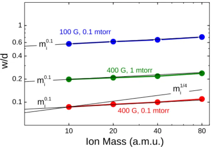
D. Scaling with ion mass
Finally, we looked at the influence of the ion mass on the leak width. Figure 17 shows the variations of the normalized leak width with ion mass for different combinations of magnetic field and pressure. It is interesting (and surprising) to note that the calculated leak width does not scale as 𝑚𝑖1/4 as suggested
by the experimental results and empirical model of Herskowitz et al. and Bosch and Merlino.
Figure 17: Leak width normalized to the distance between cusps
as a function of ion mass, 𝑚𝑖, for different combinations of
magnetic field at the dielectric surface and gas pressure. Te=2 eV,
Ti=0.5 eV. The full black lines indicate 𝑚𝑖1/4 variations
(suggested by the results of Hershkowitz et al.4 and Bosch and
Merlino12), and 𝑚
𝑖0.1 variations (best fit to the PIC MCC results
in these conditions).
Figure 18: Normalized leak width in argon at 0.1 mtorr as a function of magnetic field. The red lines and symbols corresponds to the PIC MCC simulations presented in this paper (open red symbols are the same as in Figure 14 at 0.1 mtorr and
are obtained as described in section III.G, i.e. from 𝑤 𝑑⁄ = 𝐼𝐵⁄ 𝐼0
; full red symbols are deduced from the FWHM of the simulated current density profile, which can be obtained for example from Figure 7). The blue line corresponds to the measured FWHM leak
width of Hershkowitz et al.4 (obtained from Table I of their
paper) normalized to the wire separation of 2.2 cm. The green square symbol corresponds to the measurement of Bosch and
Merlino12 in a ring cusp, normalized to the 17 cm diameter of the
ring cusp. The green triangle symbol is a corrected value of this normalized leak width, for a cusp separation of 1 cm (see text).
The variations of the leak with the ion mass 𝑚𝑖 is slower than
𝑚𝑖1/4 and close to a 𝑚𝑖0.1 law in the examples of Figure 17.
This result has been carefully checked with the three different PIC MCC simulation codes used in this paper. We do not have, at the moment a clear explanation of this result.
E. Comparisons with experiments
The scaling of the leak width with different parameters such as magnetic field, gas pressure, electron temperature can be easily compared with available experimental measurements, as done above. The values of the leak width in simulations and in different experiments are more difficult to compare because of the variety of geometry and magnetic field configurations. For example, Hershkowitz et al. used a picket fence configuration with a separation of 2.2 cm between wires, Bosch and Merlino did their experiments in a 17 cm diameter ring cusp and in a point cusp. To our knowledge the only published systematic measurements with multicusp magnets have been performed in the WiPAL plasma source and reported by Cooper et al. in Ref.11. However, as said
above, Cooper et al. presented global comparisons with previous empirical models and with a more accurate model that they developed, but did not show in this paper the variations of the measured leak width with the different parameters.
In spite of the differences in geometry and magnetic configuration of the cusps, we have plotted in Figure 18 some of the results of Refs. 4 and 12 together with our simulations
results in argon at 0.1 mtorr. First we can compare the leak
10 20 40 80 0.1 0.2 0.4 0.6 1 m1/4i m0.1i m0.1 i 400 G, 1 mtorr 400 G, 0.1 mtorr
w/d
Ion Mass (a.m.u.)
100 G, 0.1 mtorr
13 width obtained from the simulations with the definition used in the results presented above, i.e. 𝑤 𝑑⁄ = 𝐼𝐵⁄ (open red 𝐼0
symbols) with the FWHM value that can also be deduced from the simulations (full red symbols). Although the difference between the two values is not very large, we see that this difference depends on the magnetic field (because, as discussed in section III.G and as can be seen in Figure 7, the profile of the current density changes with magnetic field). The results of Hershowitz et al., which corresponds to about four times the hybrid gyroradius, are twice larger than the simulated values. Note that we compare the leak width normalized to the distance between cusps or wires although we do not know how the leak width should scale with this distance in the collisionless limit. The leak width normalized to the ring cusp diameter in the experiment of Bosch and Merlino is also shown in Figure 18 (green square symbol). Since the ring cusp diameter is large (17 cm) in this experiment, it is likely that collisions play a more important role even for this relatively low pressure conditions. In the theory of Bosch and Merlino the leak width scales with the distance between cusps 𝑑 (or the ring cusp diameter) as 𝑑1/2. Therefore, for comparisons with the 𝑑1 =1 cm case of the
simulations, the normalized leak width for 𝑑2 =17 cm should
be multiplied by √𝑑2⁄𝑑1≈ 4. This “corrected” value of the
normalized leak width is represented by the green triangle symbol in Figure 18.
It is difficult to draw any definitive conclusion from these comparisons of the values of the normalized leak width and it is clear that the comparisons of the trends (scaling laws) are more meaningful. More detailed comparisons would however be possible with the results of Ref.11 when these results are
available.
VI. CONVERGENCE AND ACCURACY OF THE
SIMULATIONS
We performed convergence tests of the simulations by increasing the number of particles per cell and the number of grid points. Figure 19 shows some examples of convergence tests for different numbers of charged particles per cell (the usual constraints of explicit PIC simulations on time step and grid spacing are satisfied).
Figure 19b corresponds to simulations with a dielectric wall (i.e. results reported in this paper). The convergence with the number of particles is satisfying and we note that steady state in the conditions of the simulations (0.1 mtorr, 400 G) is reached in a few 100 s. Most of the results presented in this paper correspond to a time around 500 s.
Figure 19a shows a convergence test with a metallic wall. Surprisingly, the convergence was much more difficult in these conditions.
Figure 19: Convergence test showing the time variations of the total electron (or ion) current collected by the wall; 0.1 mtorr, 400 G. (a): metallic wall: the number of particles per cell (ppc) is increased by a factor of two at different times of the simulation? (b), dielectric wall: three simulations with 50,100, and 200 particles per cell.
We see on this figure that each time the number of particles per cell is multiplied by two the current converges toward a larger value. It seems necessary to use a number of particles per cell larger than 800 to reach convergence. This corresponds to relatively expensive simulations in term of computation time.
We did not elucidate the reasons for the much slower convergence in the case of a metallic wall and this is one of the reasons why all the results presented in this paper correspond to a dielectric wall. Another reason for choosing a dielectric wall instead of a metallic wall in the simulations is that the electron and ion current density profiles to the wall are not identical in the case of a metallic wall so that the electron and ion leak widths are different (and their difference depends on the plasma density).
VII. CONCLUSION
In this paper we have addressed the question of confinement by magnetic cusps in a low- plasma, using 2D PIC MCC simulations. The leak width 𝑤 of a line cusp defined in the simulation is an effective loss length, i.e. in the presence of magnetic cusps, the number of particles lost to the wall per unit time is reduced by a factor 𝑤 𝑑 ⁄ with respect to the unmagnetized case. The confinement is better for lower values of 𝑤 𝑑⁄ . This definition of the leak width is slightly different from the Full Width at Half Maximum 𝑤∗ used in
experiments but is more precise and more practical for use in fluid models or global models of cusped plasma sources. The simulation results can be summarized as follows:
- In the region where the magnetic field is parallel to the wall, between the cusps, the electric potential increases from the plasma to the wall while the potential decreases from the plasma to the wall in the cusp. This forms a
0 1 2 3 5 10 0.5 1.0 1.5 5 10 400 800 200 50 ppc 100 (a) 200 100 (b) 50 ppc