Choosing the number of instruments

HB31

.M415

[DEWEY

working

paper

department

of

economics

CHOOSING

THE

NUMBER

OF

INSTRUMENTS

massachusetts

institute

of

technology

50 memorial

drive

WORKING

PAPER

DEPARTMENT

OF

ECONOMICS

CHOOSING

THE

NUMBER

OF

INSTRUMENTS

StephenG.Donald Whitney K.

Newey

No. 99-05 February, 1999

MASSACHUSEHS

INSTITUTE

OF

TECHNOLOGY

50

MEMORIAL

DRIVE

CAMBRIDGE.

MASS.

02142

Digitized

by

the

Internet

Archive

in

2011

with

funding

from

1

Introduction

There

has

been

a resurgence of interest in the application

and

properties ofinstrumental

variables (IV) estimators.

An

important

problem

in

IV

estimationis choosing the

number

of

vahd

instruments, or

more

generally a subset of all the instruments

known

to

be

valid.

The

properties ofestimators are sensitive to this choice (e.g. see

Morimune,

1983), even

in applied

work

with

many

observations (e.g. see

Bound,

Jaeger

and

Baker, 1996).

We

address this

problem by

providing simple

approximate mean-square

error

(MSE)

criteria,

that

can be minimized

to choose the instruments.

We

give these criteria for two-stage

least squares (2SLS), limited information

maximum

likelihood

(LIML),

and

the Jacknife

IV

(JIVE)

estimator of Angrist, Imbens,

and

Kreuger

(1995).

We

also

compare

the

approximate

MSE

of these estimators,

and

find

LIML

is best.

Our

criteria is

based on

higher-order asymptotic theory,

Hke

that of

Nagar

(1959),

Anderson

and

Sawa

(1979),

Morimune

(1983),

and

Rothenberg

(1983).

Our

approximate

MSE

criteria are like those of

Nagar

(1959), being

based

on

the

MSE

of leading

terms

in

an expansion

oftheestimator.This

approach

is well

known

to givethe

same

answer

as the

MSE

of leading

terms

in

an

Edgeworth

expansion,

under

suitable regularity conditions

(e.g.

Rothenberg,

1984),

and

has

been used

in

nonparametric

and

semiparametric

models

by

Andrews

(1991a), Linton (1995),

and

Powell

and

Stoker (1996). Fork-class estimators our calculations

extend

those of

Nagar

(1959)

and Rothenberg

(1983) to the misspecified

first-stage case.

We

also provide

new

results for the jacknife

IV

estimator

(JIVE)

of Angrist,

Imbens

and

Krueger

(1995).

A

number

of recent studies

have

considered the properties of

IV

estimators

when

instruments areonly

weakly

correlated with the

endogenous

right

hand

side variables. In particular

Nelson

and

Startz (1990),

Maddala and

Jeong

(1992),

Bekker

(1994),

Bound,

Jaeger

and

Baker

(1996),

and

Staiger

and

Stock (1997)

have

shown

that

standard

IV

estimators, including the

2SLS

estimator, tend to

be

biased

towards

the inconsistent

OLS

estimator

and

that inferences

based

on

2SLS

can

be

quite misleading,

when

the

mat-ter, choosing the instruments

may

help

improve

the approximation, particularly

when

the source of

weak

correlation is extraneous instruments that should

be

excluded. For example,

we show

that in data like that ofAngrist

and Krueger

(1991) our criteria will

choose the smallest

number

of instruments,

where

there is less evidence of a

problem

of

weak

correlation.

Our

criteria for choosinga subset of valid instrumentsis the estimated

MSE

ofleading

terms

in

an

expansion. This

approach

is different

than

Andrews

(1996),

who

bases

instru-ment

choice

on

the

GMM

criterion function.

We

are choosing instruments

from

a subset that is

known

to be valid while he is searching for the largest set of valid instruments.

Our

approach seems

ideally suited to

many

applications in

microeconomic

data,

where

there is a large set ofinstruments all thought to

be

valid.

Examples

include the draft

lot-tery

number

as

an

instrument for military service, as in Angrist (1990),

and

interactions of covariates with instruments, as in Angrist

and Krueger

(1991).

Our

results also apply

to the choice of nonlinear functions to use in the efficient semiparametric instrumental

variables estimator of

Newey

(1990).

Here

we

derive the optimal,

MSE

minimizing

num-ber of instruments to use, answering the important question of

how

to pick the

number

of instruments in optimal semiparametric estimation.

The

number

of instruments can

be thought

of as a

smoothing parameter

for the

nonparametric

component,

as has

been

considered

by

Linton (1995)

and

Powell

and

Stoker (1996) for other models.

In Section 2

we

describe the

IV

estimators

we

consider, present the criteria for

in-strument

choice,

and compare

these criteria for different estimators, seekingthe

one

with

smallest higher order

MSE.

In section 3

we

derive the

approximate

MSE

for

LIML,

2SLS

and

JIVE when

there are

no

covariates. Section 4 studies the properties of the criteria

theoretically

and shows

that they can

be

implemented

in a

way

that is optimal in a certain sense. Section 5 allows for covariates in the theoretical results. In section 6

we

present a

Monte-Carlo

experiment. Section 7 presents the results ofapplyingthe criteria in the Angrist

and

Krueger

(1991) appUcation.

2

The

Model,

Estimators,

and

Instrument

Selection

Criteria

The

model

that

we

consider is,

Vi

=

1^1

+

2:^/3

+

ei, E\ei\x^

=

0,V"ar(ei|xi)

=

o\, Yi

=

f{x^)

+

Ui,E[ui\xi]

=

0,Var{ui\xi)

=al,

for i

=

1, ...,N,

where

yi,

and

Yi are scalars, x, is a d

x

1 vector of

exogenous

variables,

and

Xii is a di

X

1 vector of

exogenous

variables

which

are

assumed

to

be

a subset of

Xi,

where

we

assume

homoskedasticity throughout.

We

also

assume

that conditional

third

moments

are zero

throughout

the paper.

The

first equation is the equation of

interest

and

the right

hand

side variable Yi is possibly correlated with e, so thatgenerally E{uiei\xi)

=

aue 7^ 0,

The

second equation represents the

reduced

form

relationship

between

Yi

and

the

exogenous

variables Xi

which

is allowed to

be

nonparametric, with

f{xi)

=

E{Yi\x,).

Because

oftheconditional

moment

restriction E{ei\xi)

—

0, functions ofXj

can be used

as instrumentsinestimating the equationofinterest. Letipf

=

(ipiKi^i),

,4'KK{^i))' be

a vectorof

K

functions to

be

used asinstrumental variables,

where

we assume

throughout

that xpf" includes Xu.

They

could

be

approximating

functions, such as

power

series

or regression splines, as in

Newey

(1990).

The

problem

we

consider is

how

to choose

this instrument vector so that the associated

IV

estimators

have

good

properties. For

simplicity

we

have

allowed

K

to serve as

both

the

number

of instruments

and

the index

of the instruments, but

we

could proceed

more

generally

by

specifying a different index

for the instruments. If

we

did that the criteria could

be

used to

compare

instrumental

variables estimators with the

same

number

of instruments.

We

consider several different

IV

estimators.

To

describe

them

let

^^ =

[ip^

,...,ip^]'

be

the

matrix

ofobservations

on

the instrumentalvariables,

P^

=

^'^(^^'^'^)~i^-'^' the

associated projection _{matrix, y}

=

_{(yi, ...,yn)',}

Y

=

(Yi, ...,y„)',

Xi

=

[xn, ...,Xin]',

W

=

overA,

where

Pi

=

Xi(XjXi)

^X[.

The main

class ofestimators considered is the k-class

which

includes estimators

which have

the form,

6={{1

+ k)W'P^W

- kW'W)-\{1

+

K)W'P^y -

nWy)

where

the scalar

k

is given by,

ad

₊

j^

K

=

l-a9-j^

for constants a

and

b. This class of estimators includes

2SLS,

where

a

=

b

=

0,

LIML,

where

a

=

1

and

6

=

0,

and

a bias-corrected

2SLS

estimator like that of

Nagar

(1959),

denoted

here

by

B2SLS,

where

a

=

and

b

=

K

—

(2

+

di). This class of estimators is

similar to that considered

by

Rothenberg

(1983).

The

other estimator considered is the Jackknife

IV

estimator

(JIVE)

proposed

by

Angrist,

Imbens

and Krueger

(1995). It has the form,

(

IJ

\

_

{

y'C'Y

Y'C'X,

\

~

Y

Y'C'y \

[Pj

)-[

X[Y

X[X,

)

[X[y

)

where

C

is the matrix with Cij

=

Pij/{1

—

Pa) for i 7^ j

and

Cu

=

0.

Note

that

CY

has the interpretation as the vector of predictions of the Yi given all but the ith observation,

hence

the Jackknife terminology.

The

instrument selection criteria are

based

on

the

approximate

mean

square error

(MSE)

for the

endogenous

variable coefficient estimator 7.

Implementing

these criteria

requires preliminary estimates of

some

of the parameters ofthe

model

and

a

goodness

of

fit criteria for estimation ofthe reduced

form

using the instruments ipf. Let 6 denote a

preliminary

IV

estimator

and

let e

=

_y

—

W6.

Also, let

u

denote

some

preliminary

reduced

form

residual estimator, such as that obtained

from

the residuals

from

the regression of

y

on

^^

for

some

fixed

K.

Then

let

o-,^

=

e'e/N,_al

=

u'u/N,

_Uu^

=

u'e/N.

It is

important

in

what

follows that

none

ofthese preliminary estimators

depend

on

K.

For

example

S

might be an

IV

estimator with just one instrument for Yi, or it

might be

offit criteria given below. Similarly, the

reduced

form

residual

u

might be from

the first

stage regression

with

the best fit. In

any

case these estimates

must

remain

fixed as the

criteria for different instruments sets is calculated.

The

reduced form goodness

offit criteria can

be

formed

in at least

two

ways. Let

u^

denote

the

reduced form

residual vector

from

regressing

Y

on'^^

.

The

Mallows goodness

of fit criterion for the

reduced form

is

R{K)

=

{u^'u^/N){l

+

_~^)

The

cross-validation

goodness

of fit

measure

is

^f)

2

Eitherofthese will

have

suitabletheoretical properties forusein theinstrument selection

criteria.

The

preliminary estimatesofcovariance

parameters

can be

combined

with

the

reduced

form goodness

of fit

measures

to

form

criteria for the choice of instruments for

each

of

2SLS,

LIML,

and

JIVE

as

S2SLs{K)

=

al^

+

aUR{K)

- al^)

suml{k)

=

^![m)~^^)

For each estimator, choosing

K

to

minimize

the corresponding

S{K)

will result in

₇

that has relatively small

MSE

asymptotically.

These

criteria also will apply

when

K

is not

the sole index of the instruments, e.g. for

comparing two

different sets of instruments that

have

the

same

number

ofinstruments.

Choosing

the estimator

where

the expression

on

the right-hand side is smallest will result in the best

asymptotic

MSE

in that case as well.

It is interesting to

compare

the size of the criteria for different estimators,

because

LIML

and

JIVE

criteria are

both

of smaller order

than

the

2SLS

criteria. This reflects

that the bias of

2SLS

increases with the

number

ofinstruments at a higher rate

than

the

other estimators, a result previously established

by

Morimune

(1983). Consequently, for

large

numbers

of instruments

both

LIML

and

JIVE

should

dominate

2SLS

in

terms

of

MSE.

Also, the criteria for

LIML

is smaller

than

that for

JIVE,

so that

LIML

is best

among

these three estimators.

As

previously

shown

by Rothenberg

(1983) for the fixed

instrument case, it turns out that

LIML

is best

median

unbiasedto the order

we

consider

in the k-class of estimators.

3

The

Mean

Square

Error

For

much

of this section

we

focus

on

the simplest

model

which

is a special case of the

model

considered in Section 2. In particular

we

focus

on

the model:

Vi

=

lYi

+

Ci Yi

=

f{x,)

+

Ui

forz

=

I, ...,N,

where

yi,Y^

and

e, are all scalars

and where

Yi is possibly correlated with

Cj. In Section 3.5

below

we

show

how

the

MSE

criteria

can

be extended

to

models

with

covariates as considered in Section 2. In this case, the estimator for

₇

is given by,

7

=

((1

+

K,)Y'PY

-

kY'Y)-\{1

+

K)Y'Py

-

KY'y)

where,

l-a9-j^

_N

with

6 being the

minimum

value of, X'Y'

PY

X/

X'Y'Y

\.

The

other specific estimator considered is

JIVE, which

is

denoted

by,

7j

=

(Y'C'Yy^Y'C'y

where

C

was

described in Section 2. Unfortunately

JIVE

does not

appear

to fit into the k-class of estimators so that

MSE

calculations will

have

to

be

performed

separately.

3.1

Calculation

Our

approach

to finding the

approximate

MSE

is similar to that of

Nagar

(1959). First

we

normahze

the estimator (let

7

denote a generic estimator),

ViV(7-7)

=H-^h

where

H

and

h

are different for different estimators

and

have

population counterparts,

h

=

i/'e

and

Then we

use the expansion.

„_f'f

H-'h

=

[{I

-{H-H)H-^)H]-\h +

Ch-h))

=

H-\h

+{H

- H)H-^h

+{H-

H)H-\h

-

h)

+

{H

-

_HfR-'^h

+

...

and

note that since

H"^

is a

common

factor for all

terms

in the expansion, Ave

can

calculate

an approximate

MSE

by

taking expectations of the square of the expression,

Hy/N{^-^)

=

h

+

{H-H)H^^h

+{H

-

_H)H-\h

-h)

+

{H-

HfH-'^h

+

...

Then

following

Nagar

(1959)

we

find the

MSE

of this expression using the largest (in

probability)

terms

inthe squareofthisexpression, althoughsince

we

are interestedin the

selection of

K

and

allow

K

—

>• 00

we

include only thoseleading

terms

in the

MSE

that are

pertinent tothe choice of

K

for the estimator of interest.

Thus

terms

that

do

not

depend

on

K

will

be

omitted.

Because

of this fact,

terms

beyond

the

second

willnot (ingeneral)

contribute to the

approximate

MSE

criteria to

be used

for selection of

K

, even

though

they

do

contribute to the

MSE

in the case

where

one has a fixed

K

and

one

obtains

an

approximation

to the

MSE

to

0{\/N).

For the purposes of completeness

and

to enable other types of

comparisons

we

also provide

approximate

0{1/N)

MSE

calculations for

fixed

K. These

calculations extend the

work

of

Nagar

(1959)

and

Rothenberg

(1983) to

the case

where

there is a possible misspecification in the first stage. In such a calculation

the third

and

fourth terms

do

contribute to the

approximate

(to

0{\/N)) MSE.^

Note

that the leading

term

(which is ₀₍₁₎₎ in the

approximate

MSE

will

be

E{hh!)

=

a'J-^

and

that this will

be

common

to all of our

approximate

MSB's.

Since this

term

has

no

bearing

on

the choice of

K

and

since it is

common

to all of our estimators

we

omit

the

term from

the expressions

we

present

and

focus

on

the

remaining

terms. All calculations are

done

conditional

on

the

exogenous

variables Xi,

The

assumptions which

are used to derive

an approximate

MSE

are

now

stated

and

discussed.

Assumption

1

Assume

that {xi,Ui,ei] are iid,

and

satisfy,

(i) E{u^\xi)

=

E{ei\x^)

=

0,

(ii)

<

E{uf\xi)

=

al

<

oo

and

<

E{ej\xi)

=

a^

<

oo,

(in) E{ui'ei^\xi)

=

0, for

j+

k being a positive

odd

integer such that k

+

j

<

5,

(iv) E{\ui\^\ei\^\xi)

<

oo, for

any

positive integers j

and

k such that k

+

j

<

5,

(v) Xi have support

X

C

R^

that is the Cartesian product of

compact

intervals.

Assumption

l(i)

was noted

in Section 2.

Assumption

l(ii) is a homoskedasticity

assump-tion that simplifies the calculations while

Assumption

l(iii) is a

symmetry

assumption

which

implies that

both

residuals

have

symmetric

distributions. This will

be

satisfied if

theresiduals arejointly

normally

distributed.

Assumption

l(iv) requires the existence of

at least five

moments

for the residuals.

Assumption

l(v) is standard in the literature

on

series

based

nonparametric

regression.

The

next

Assumption

concerns the nature of the

optimal instrument function /.

Assumption

2

The

function f{xi)

=

E{Yi\xi) is such that,

(i)

_f

:

X

-^

R

and

has

an

extension to all of

R^

that is s

>

times continuously

differentiable in x,

(a) with probability 1,

<

c

<

N~^

'^^^-^ f{xi)'^

<

c~^ for

some

small constant c

uniformly in

N

.

Assiimption 2(i) is a

smoothness

condition that allows one to obtain

approximation

rates for series

based

methods.

The

second part of this

assumption

is

an

identification

assumption

that requires that /(xj) not

be

identicallyzero

which

would

result in

7

being

unidentified. This will

be

modified

when we

consider the introduction of covariates into

the structural equation.

Assumption

3: Letting

Pa

denote the ith diagonal element of

P,

assume

that

sup

Pu

-^

i<7V

as

N

^>- _{00 withprobability one.}

It should

be

stressed that this

assumption

is not required for

one

to

show

that

yN{'y

—

'y) is asymptotically normal,

and

is only necessary to obtain tractable expressions for the

MSE.

It requires

some

restrictions

on

the rate at

which

K

increases

with

the

sample

size

that are

much

stronger

than

those

needed

to

show

asymptotic normalityoftheestimators.

It should

be noted

however

that as long as s in

Assumption

3 is sufficiently large the

restrictions will allow for

K

to increase at a rate that results in the fastest possible rate ofconvergence ofthe

MSE

expression to zero.^

Our

first result gives

an approximation

to the

MSE

for a subclass of the k-class

estimators

we

are considering. In obtaining all ofour

approximations

we

have

restricted attention to k-class estimators that

have

values of a

and

b that satisfy certain properties. In particular it is

assumed

that a

=

0(1)

while b

=

0{K),

which

includes all of the Donald(1997) hasshownthatforpowerseriesonerequiresthat

K^/N

—

>

when

Xi hasa continuous

estimators

mentioned above and

ensures that the estimators will

be

consistent.'^

The

first subclass of estimators consists of those for

which

the

approximate

bias (to order

N~^^'^) is increasing in

K.

Unless otherwise stated all

MSE

will refer to the

terms

in the large

sample

large

K

MSE

that are

dominant

amongst

those that increase

with

K

and

those that decrease with

K.

Proposition

1

Given Assumptions

1-3,

assuming

that a

—

₀₍₁₎

and

b

=

0{K)

such

that {l

—

a)

— b/K

is

bounded

away

from

_0, the

MSE

for

\/N{'y—^)

is approximately

[{l-a)K~bf

,

,f'{I-P)f

crL-

_U€

_h

+

(y.

N

'

N

It is straightforward to

show

that the

approximate

bias, to

0{N

^/^) _{is of the form^}

[(l_a)/<-6-(2-a)]a„,

_ff'fY'

/TV

\N

•

^^-^

and

that for estimators in the class

under

consideration

whose

bias

term grows with

K

,

the leading

term

in the

MSE

comes

directly

from

the squareof this bias.

The

second

term

in our

approximate

MSE

comes from

the

approximation

error inherent in the estimation

of

/ by

a series

based

approximation.

The

result in Proposition 1 leads directly to

an

approximate

MSE

for

2SLS

which

is the only estimator

under

consideration

which

falls

into this class.

Corollary

1

For 2SLS,

_72, which has a

=

and

6

=

0, the approximate

MSE

of

^(72 —

7),

under Assumptions

1-3, is given by,

,

K^

J'{I-P)f

ut

_N

'

N

Notethat,aswillbeseen,theseconditionsontheirowndonot ensureroot-Nconsistency. Ingeneral this will require restrictionson therate of increase ofK.

''See Rothenberg (1983) forexample. Also note that the expression forthebias isthesame asNagar

The

result in Proposition 1 does not reveal the large

K

approximate

MSE

for either

LIML

or

B2SLS

because neither of these estimators

have

a bias (to 0{N^^^'^)) that

depends on

K. Thus

we

need

to provide

an

additional result that will yield

approximate

MSE's

for such estimators.

Proposition

2

Given Assumptions

1-3,

assuming

that a

=

0(1)

and

b

=

0{K)

such

that (1

—

a)K —

b

=

0(1), the

MSE

for •\/iV(7

—

₇₎ is approximately

{K -

2aK

-

2ab)

K

J'{I

-

P)f

"^

_N

"^

_"^

A^ '

N

This

result

can

be used

to obtain

approximate

MSE's

for

LIML

and B2SLS.

Corollary

2

For

LIML,

'Jl,'whichhas a

=

1

and

b

=

0, the

approximate

MSE

Jory/N{'^L—

7)

under

Assumptions

1-3, is given by,

K^.

-0^+^.

—

-^

—

Corollary

3

For

B2SLS,

_'^b,"which has a

=

and

b

=

K

—

2, the

approximate

MSE

for\fN{ffs

~

7)

under

Assumption

1-3, is given by,

/ 2 2

2^K

J'{I-P)f

The

expressions derived thus far

do

not allow

one

to derive a criteria for

JIVE.

Interestingly, the following result

shows

that

JIVE

has the

same

MSE

expression as

B2SLS.

Proposition

3

For JIVE,

7j, the approximate

MSE

fory/N{'yj

—

7) is given by

3.2

Discussion

Some

insight into the differences

between

the

approximate

MSE

for the estimators can

be

gained

by

looking at the

terms

in theexpansionofeach that contributes to the leading

terms

in the

MSE

expressions. For

2SLS

this

term

has the form,

'Pe 1

/

^

AT

w

\

where

thefirst

term on

the rightreflectspartofthebiasthat occurs

due

totheendogeneity

in the

model

(i.e. correlation of Ui

and

e,)

and

which grows

with K.^

The

square of this

bias

term

gives the leading

term

in the

MSE

for

2SLS.

The

variance of the

complete

expression contributes

0{K/N)

terms to the

MSE,

and

these are

dominated by

the

leading bias squared term.

Both

LIML

and

B2SLS

have the leading bias

term

(which

depends

on

K)

removed

and

so the leading

terms

in their

MSE

come

from

the variance

terms.

An

alternative derivation of

LIML

shows

how

this bias reduction occurs. In particular the

LIML

estimator 7/, can

be

shown

to

be

the solution to the following

problem,

mm

^^

where

Y

=

{y,Y),

and

7;^

=

(1,-7).

Given

this, it is straightforward to

show

that the

LIML

estimator satisfies the following first order condition,

where

e{f)i)

=

_U

~ IlY

Letting,

y'<iL)

KlL)

=

we

can rewrite the first order condition as,

1

(F-<5(7je(7L))'Pe(7L)

=

0. ₍₃₎

Since 6 can

be

interpreted as being the coefficient in the

hnear

regression of

y

on

e the

first

term

in the

above

can

be viewed

as being the residual

from

this regression,

which

should then not

be

linearly related to e.

Thus

the

term

for

LIML

that corresponds to (2)

has the form,

1 v'Pe

=

-. /

N

N

N

\

-=

I

Y^

v^SiPu

+

J2Y1

""^^^-^v 1 (4)

/N

where, O-ue Vi

=

Ui -Ci

is

by

construction rmcorrelated with Cj.

Note

also that the leading

term

in the

MSE

expression for

LIML

is equivalent to, cr^cr^.

The

term

for

B2SLS

corresponding to (2)

and

(4) is equal to,

(3)

Vn

^ f

N

N

N

\

where

the leading

term

has,

by

construction, zero expectation. This, again, results in a lower order leading

term

in the

MSE

for

B2SLS.

The

lower leading

term

for

LIML

compared

tothat of

B2SLS

comes about because

ofthe lower variance that arises

because

Vi is rmcorrelated

with

ej

and

because Vi has a lower variance

than

tij. Finally, it is easy

to see

why

JIVE

has the

same

leading

term

as

B2SLS,

sincefor

JIVE

the expression that

is analogous to (2), (4)

and

(5) has the form,

in

1 /

^

^

2^2^zx,e,Q,

(6)

v^

v^

_{V.=l ,^.}

which

has zero expectation. This expression results

because

of the use of the Jackknife

in the first stage.

3.3

Further

Comparisons

Our

discussionthus farhasindicated that,in termsof

dominant terms

inthe

approximate

(large

K) MSE,

LIML

dominates

JIVE

and

B2SLS

and

that all of these estimators

dominate

2SLS

because of the larger order (in

K)

leading

term

of the latter.

Another

type of

comparison

that can

be

made

is in terms of the

MSE

for a fixed value of

K

for which, generally speaking, the chosen instrument set

may

be

suboptimal.

The

nice feature ofthis comparison, is thatifthe expansion is taken

up

to

terms

oforder

N~^

then

one

can see clearly the

opposing

effects ofincreasing

K

more

clearly. In addition such

an

expansion extends the

work

of

Nagar

(1959)

and Rothenberg

(1983) to the misspecified

first stage case

and

may

reveal

any

potential differences

between

estimators

when

one

uses

an

imperfect fixed set of fixed instruments in the first stage. ^

Proposition

4:

Given Assumptions

1, 2(i), 3,

assuming

that a,b

and

K

are fixed

and

that (for

some

small constant c),

f'-Pf 1

0<c<

^-—^ <c-^

N

with probability 1, uniformly in N, then the

MSE

for

viV(7

—

7) using

terms

up

to those of

0{N~^)

is approximately

2lf'PfY\

2

[{l-a)K-b]'

ff'Pf^-'

N

J ""'

N

\

N

^ 2 ,

{{K-2aK-2ab)-8[{l-a)K-b]}

\ /

fPp

"' "^ I

N

J \

N

, , .

{K-2[{l-a)K-b]}

\

ff'Pf

„

,'12-

Aa-a^\

ff'PfY^

_, ,

/4

-

2a\

ff'Pf

-2

+2a

,,a{K-l)

+ b\f'{I-P)f

ff'Pf

N

N

\

N

The

conditions used to derive the expression in Proposition 4 are the

same

as

used

previously except that

we

have

introduced a condition that modifies

Assumption

2(ii) to

^Indeed our result reduces to that of Nagar (1959) in theperfect first stagecase when o

=

as he

assumed. The expression obtained in Proposition 4 does differ from the

MSE

expression one obtains

fromTheorem 2 ofRothenberg (1983). Additionally, inthe a

=

case, the expression oneobtains from Rothenberg (1983) is not consistent with that obtained by Nagar (1959). The difference between that obtained from Rothenberg (1983) and Nagar (1959) andours is minorand appears appearto bedue to

typographical error in thestatement ofTheorem 2 ofRothenberg (1983). Indeed asingle sign change

ensure identification in the fixed

K

case.

Note

that the leading

term

in this expression,

when

taken to the Hmit, is the asymptotic variance of the estimator,

when

K

is fixed.

When

K

is fixed

and

when

the instruments are imperfect (in the sense that they

cannot

predict

_/

perfectly) then it is the case that,

since /'(/

—

P)f

>

which

follows because /

—

P

is positive semidefinite. In fact

if the instruments are imperfect (in the sense that they

cannot

predict

_/

perfectly)

then

it is the case that the inequality is strict.

Note

that the expression

on

the right

of the inequality is the lowest variance possible for this particular problem.

Given

the expressionin Proposition4,

one

can then see clearly that increasing

K

will

have opposing

effects. First, increasing

K

will cause the limiting variance to

be

closer to the optimal

approximate

variance for the estimator.

That

is,

because

when

K

-^ oo then

by

Assumption

2, f'{I

—

P)f/N

-^ 0.

On

the other

hand

the

other

terms

will generally increase.

Our

expressions derived earlier, involve the largest

terms

reflecting each of these effects.

The

optimal choice of

K

, then, will

be

the

one

that balances these

two opposing

effects.

The

expression in Proposition 4 can also

be used

to

compare

the different estimators

in the class

under

consideration. In particular the

approximate

MSE

for

2SLS

is,

^^

1,^

+

r-

[

—

N

—

)

+^"^^^^/

[-^r)

for

LIML

we

have,

and

finally for

B2SLS

we

have,

To

allow

comparisons

ofthese k-class estimators with

JIVE

inthe fixed

K

case

we

derive

the appropriate

MSE

expression for

JIVE

below

in Proposition 5.

Proposition

5:

Given Assumptions

1, 2(i), 3,

assuming

that a, b

and

K

are fixed,

supjPii

=

0{N~^)

and

that,

0<c<^<c-i

iV

with probability 1, uniformly in N, then the

MSE

for \/iV(7j

—

7) using

terms

up

to those

ofO{N-^)

fPfV

, ..2 ,

..J<

ff'P'fV"

, ,,0.2 , . . 2x 1

ff'P'f

a'

(^)

.«..x,f(^)-.(i..i...>n^(^)

^^^,,ni-p)p{i-p)f\

ff'P'f

-2

N

\

N

Note

the additional condition in the statement ofthe result

which

concerns the rate

at

which

the largest diagonal of the matrix

P

goes to zero

which

is a strengthening of

Assumption

3

and

is not

needed

for

any

other result. Itis fairlyeasytoprovideconditions

thatjustify this conditionin the fixed

K

case considered in the result

-

for instance given

that

Assumption

2 holds one

can

verify this condition if the smallest eigenvalue of the

matrix

"^'"^

/N

is

bounded away

from

zero.

The

reason for

imposing

this condition is to get

an

estimate of,

'f'PfY^

ff'C'f\

"^

f'C'Cf ff'C'f\

"^

N

J \

N

J

N

\

N

where

the complicated

form

for

JIVE

comes from

the use of the Jackknife in the first

stage,

and

similar to the results for

LIML

and B2SLS,

introduces

an

additional

0{N~^),

term

in the

MSE.

Such an

additional

term

does not

appear

in the expression for

2SLS.

the variances

and

covariances but also

on

the degree ofmisspecification ofthe first stage.

It is interesting to notethat althoughthis misspecificationobviously affects allestimators

through

the leading

term

(the

approximate

variance) it also affects

LIML,

B2SLS

and

JIVE

in the smaller order terms. Indeed

one

could envision scenarios

where

K

is fixed

at

some

large

number

and

where

there is still a great deal of misspecification in the first

stage - _{in such a scenario} it

may

be

possible for the final

term

in the

MSE

for

LIML,

B2SLS

and

JIVE

to

be

large

and

indicate

poor

behavior of these estimators relative to

2SLS.

One

can

do

more

general

comparisons

of the estimators in the case

where

there is

a correct specification in the first stage so that

Pf

=

_f

. In this case the last

terms

in

the

MSE

for

LIML,

B2SLS

and

JIVE

would be

omitted.

Comparing

the resulting

MSE

reveals that although

JIVE

and

B2SLS

have

similar bias reduction properties

and

the

same

criteria for picking

K,

B2SLS

appears to

be

superior

with

respect to

terms

that

do

not

depend

on

K

(at least using the

approximate

MSE

to

0{N~^)).

A

comparison

of

the

MSE

for

LIML

and

B2SLS

reveals that

LIML

has a lower

MSE.

The

comparison

of

2SLS

with

the other estimators

depends

on

the variances

and

covariances in the model.

Not

surprisingly large (fixed) values of

K

and

reasonable levels of covariance

between

the

residuals

would tend

to lead to superior

MSE

for the other estimators relative to

2SLS.

The

expressions in Propositions 4

and

5 also

makes

it possible to consider

what

happens

when

there is

no

endogeneity problem, so that aue

=

0.

When

aue

=

0, the

optimal

number

of instruments for

JIVE

and

B2SLS,

using the criteria

developed

in

Section 3.2, is exactly the

same

as for

LIML,

which

is equal to the optimal

number

of

terms

required forestimating

/

in thefirst stage.

On

the otherhand, the

MSE

expression

just given for

2SLS,

(when

a^e

=

0) is monotonically decreasing in

K

which

indicates

that the optimal choice of

K

is as large as possible. This, not surprisingly,

makes

2SLS

identical to

OLS, and

is

due

to the fact that

when

a^^

=

0,

OLS

is the Best Linear

Unbiased

Estimator.

The

reason that this does not occur

with

LIML

is that the

LIML

estimator

would

no

longer

be

defined

when

there areas

many

instruments as observations while the delete-one nature of the first stage

used

in

JIVE

makes

first stage predictions

based on

as

many

instruments as observations very unreliable.

Because

ofthe

dependence

of

comparisons

on

the degree ofcorrelation

between

resid-uals, it is difficult to use the expressions in Propositions 2

and

4 to derive

an

convenient optimal estimator in the class

under

consideration. It is possible,

however

to describe

the optimal estimator for classes of estimators that

have

similar bias properties.^

The

first result will use the expression in Proposition 2 to give a class of estimators that are

optimal with respect to the large

sample

large

K

MSE

to order

K/N. The

class

under

consideration consists of those estimators

whose

bias is of 0{N~^''^) (and

hence have

a

squared

bias of

0{N^^))

which, as

noted

earlier, places restrictions

on

a

and

b that rule

out

2SLS

but include

LIML

and

B2SLS

as possibilities. This result is stated

below

in

Lemma

1

and

is

an immediate consequence

of Proposition 2.

Lemma

1 In the case

where

K

^

oo in such a

way

that {l

— a)K —

b

=

_0(1), the optimal

estimator, with respect to the large

sample

(large

K)

MSE

to

0{K/N)

must

have a

=

\

and

b

=

0(1).

Note

that this result does not pin

down

a single estimator, since

one

can pick

any

constant value for b

and

still

have

the

same

leading

terms

in the

MSE

expansion, since

terms

involving

K/N

will

dominate

those of

0{N~^)

for large

K.

It does suggest,

how-ever, that

LIML,

being

one

such estimator, will

have

better (large

K)

MSE

properties

than

the other estimators

under

consideration. Note, again, that

2SLS

does not fit into

the class of estimators

under

consideration because its bias is not 0{N~^''^) (again as

K

—> _oo) as the condition in the result requires.

The

next result is for the class of

estimators that are unbiased to 0{N^^/'^)

and

follows similarly

from

Proposition 2.

Lemma

2 Restricting attentionto estimators that are suchthat (1

—

a)/C

—

6—

(2

—

a)

=

0,

the optimal estimator, with respect to the large

sample

large

K

MSE

to

0{K/N)

must

have a

=

1

and

consequently 6

=

1.

''Indeed this was done by Rothenberg (1983) for theclass of(approximately) median unbiased esti-mators, in which

LIML

was optimal.

This result states that the optimal estimator in the class of estimators that are

unbi-ased to 0{N~^/'^) is thebias adjusted

LIML

estimator. It should

be

noted, however, that

for such

an

estimator the optimal choice of

K

is completely unaffected

by

the bias

ad-justment

and

that the criteria for choosing

K

will

be

identical tothat obtained for

LIML.

A

similar result to that in

Lemma

2 is obtained

when

one

assumes

that

K

is fixed

and

considers

approximately

mean

unbiased estimators with

M3E

given

by

the expression in

Proposition 4.

Lemma

3

Restricting attention to estimators that are such that {l

— a)K—b—{2—a)

=

0,

theoptimal estimator, withrespect to the large

sample

fixed

K

MSE

to

0{N~^)

must

have

a

=

1

and

consequently 6

=

1.

This result

shows

that

when

there is misspecification in the first stage (as

happens

in general

with

K

fixed) the bias adjusted LIA-IL estimator is optimal

with

respect to

the

MSE

to

0{N~^).

This is a

minor

extension, to the misspecified first stage case, of

the conclusions

one

draws

from Rothenberg

(1983) concerning the optimality of the bias

adjusted

LIML

estimator

among

the classof

approximately

mean

unbiased

estimators. In

additionto this,

Rothenberg

(1983)

showed

that forfixed

K

and

a correctly specified first

stage

LIML

is optimal (with respect to the

MSE

to

0{N~^))

among

all (approximately)

median

unbiased

estimators.

Thus

based on both

the

dominant terms

in large

K

MSE

and

peripheral or second order terms there appears to

be

ample

evidence to suggest the use of

LIML

or bias adjusted

LIML.

3.4

Admitting

Covariates

In this section

we

generalize the results to the model,

Vi

=

lYi

+

x\iP

+

e

where

x^

is a rfj

x

1 subvectorofx^.

The

most

important

difference that arisesinthe

more

/5i)'-However,

it

can

be

shown

that the

MSE

of estimators of Pi are directly

and

positively

related to the

MSE

of estimators of 7. In particular,

assuming

that

Xu

is included in

the instrument set (which

would be

the case if one were using

power

series) then

any

estimator of/^jwill

have

the form,

where

Xi

denotes the

N

x

di matrix with zth

row

qual to Xu. ^ _{Since for all three}

estimators the

MSE

_{of Pi}

depends

on

K

only

through

its

dependence on

_7,

we

can

focus directly

on

the

MSE

of the

₇

in each case.

When

covariates are present the estimators

of

₇

take the form,

7

=

((1

+

k)Y*'PY*

-

kY*'Y*)-\{1

+

K)Y*'Py

-

KY*'y)

where

Y*

=

[I

—

Pi)Y

with Pi being the projection matrix

formed

using Xi.

The

JIVE

estimator will take the form,

^j

=

{Y'C'{I

-

Pi)YY'Y'C'{l

-

Pi)y.

Before presenting the

MSE

calculations

we

modify

Assumption

2 as follows, letting tt

denote the population regression coefficients

from

the regression of Yi

on

Xu.

Assumption

2'

_The

function f{xi)

=

E{yi\xi) is such that,

(i)

_f

:

X

^

R

and

has

an

extension to all of

W^

that is s

>

times continuously

differentiahle in

x

and,

(a) with probability 1

<

c

<

N~^

_X]i=i(/(^i)

~

^'u^)'^

<

^~^ /'^'^

some

small constant

c uniformly in

N

(Hi) the smallest eigenvalue of

X'lXi/N

is

bounded

away from

zero uniformly in

N

with probability one.

The

adjustments

in

Assumption

3' are

due

to thefactthat theidentification condition

now

suggests that Xi explain Xji

beyond

that provided

by

a

hnear

regression

on

x^.

^

The new

condition (iii) along with

Assumption

l(v) is

used

to

bound

the elements ofthe

vector, (/

—

Pi)/

and

the variances

and

covariances ofelementsof[I

—

Pi)u

and

[I

—

P\)e.

Indeed

these conditions ensure that the variance of a typical element of (/

—

Pi)u, say

Ui

—

P'liU (with Pii denoting

column

i of Pi), is equal to that ofw, plus a

term

that is

0{N~^)

and

that

any

covariances

between

these elementsare of

second

order importance.

The

same

holds true for the vector (/

—

Pi)e

and

for covariances

between

these vectors.

Once

this has

been noted

one can obtain large

K

MSE

expressions for the estimators

of interest that are the

same

as in the case of

no

covariates provided that the set basis

functions

used

as instruments contain linear

terms

in Xu.

Corollary

4

Given

Assumptions

1,2'

and

3 plus

PPi

=

Pi the conclusions of

Corol-laries 1, 2

and 3 and

Proposition

3

all hold.

It is easy to see

why

this result holds

when PPi

=

Pi.

The

only difference that

would

obtain

by

allowing for

exogenous

covariates in the equation

would

be

that the

second

terms

in the

approximate

MSE

would have

the form,

/'(/

-

Pi)(/

-

P)(/

-

Pi)//A^

=

/'(/

-

P)/

where

the equality

comes from

the fact that

PPi

=

P\.

A

simple

consequence

of this result is that rules for choosing

K

and

any optimahty

results discussed previously

apply

carry over to the situation

with

covariates.

4

Feasible

Optimal

Estimation

of

K

In this section

we

consider the properties of the estimated

MSE

criteria discussed in

Section 2.

Throughout

this section

we

will use the following

assumptions

concerning the preliminary estimation of the parameters, o"^, o"^

and

a^^.

®This is essentially a relevance condition and Donald (1997) has considered tests for the failure of this condition in contexts wherethere are anarbitrary numberof righthand sideendogenousvariables.

Assumption

4

Assume

thefollowing,

(^) _^l

-

ol,

(n) al

^

al

(Hi) Gut -^

O-uc-As

noted

in Section 2, this can

be

achieved

by

using

some

prehminary

set of estimates

of the

model

obtained

by

using the

number

of instruments that provide the optimal fit

in the first stage,

based

on

either the cross-validation or

Mallows

criteria.

Note

that the

other key ingredient used to

form

the estimated criteria is

R{K)

which

can either

be

based

on

cross validation or the

Mallows

criteria as discussedin Section 2. Li (1987) has

shown

that each of these criteria are asymptotically optimal in the sense that the value of

K

that minimizes these criteria,

denoted

K,

satisfies the condition,

RJK)

, .

infx /?(/<) '

in probability.^° _{For a generic estimator}

₇

_{with estimated criteria}

_S{K)

_and

_{true criteria}

S{K) we

will define the data driven optimal choice of the

number

ofinstruments by,

K

=

argminS{K).

The

minimum

and

all

infimum

will

be

relative to

an

index set of

K

values,

which

may

require

some

restrictions in order to prove certain results. Also, notice that although

R{K)

only estimates

R{K)

up

to a constant,

which

does not

depend

on K, one

can

remove

this constant

from

R{K)

and hence from

S{K)

without affecting the choice of

K.

To

analyze the properties of

K

we

follow the

approach

of Li (1987)

and

Andrews

(1991b). In our case

we

use the following definition of optimality.

Definition:

A

method

ofselecting

K

is defined to he "higher order asymptotically

opti-mal

with respect to the criteria

S{K)

" _ifit can be

shown

that,

s{k)

,

inf;,5(/^)

^"Andrews (1991) proved the same results for appropriate adaptations ofthese criteria in the case

The

use of the

term

"higher order" is necessitated

by

the fact that the optimal

MSE

convergence rate in all cases will

be

A'^"^ (as

N

—

> oo)

which

cannot

be improved upon,

and

the criteria

based

on

S{K)

concerns thenext largest

terms

inthe

MSE

that

depend

on

the choice of

K.

A

vital step in

showing

that the criteria are higher order

asymptotically-optimal, is

showing

that

R{K)

consistently estimates

R{K)

up

to the constant in the sense that, in probability,

This is the condition

used

by

Li (1987) to

show

the

asymptotic

optimalityofthe

Mallows

criteria

and

cross validation. Inorderto

be

able toverify this result

we employ

conditions

similar to those of Li (1987).

Assumption

5:

Assume

that thefollowing conditions hold,

(i) E{u\\xi)

<

oo

and

(a) inf^

NR{K)

-^ oo,

and

in addition

when

R{K)

is the cross validation criteria,

assume

(Hi) the index set satisfies the condition that

sup^

sup^F^j -^ in probability.

The

conditions (i)

and

(ii) in

Assumption

5 are

needed

for

both

the

Mallows

criteria

and

cross validation, to

show

that they satisfy (7).

These were

employed by

Li (1987) to

show

that these criteria are asymptotically optimal. Here, this is

an

intermediate step to

showing

higher order

asymptotic

optimality.

The

second of these requires either that

_/

not

have

a finiteorder representationin

terms

ofthebasis functions orelse that the lower

bound

on

the set of

K

values over

which one

is doing the minimization

grows with

A'^,

which

is

perhaps

undesirable

from

a practical standpoint.

The

condition (iii) is required

only forthe cross validation

based

method,

and

is similar to the conditionin

Assumption

upper

bound

on

the rate at

which

the index set can

grow

with the

sample

size ^^

The

followingresults

show

that for each estimator the estimated criteria provides a

means

to

obtain higher order asymptotically optimal choices for the

number

of instruments.

Proposition

6:

Given Assumptions

4 o-'^d _5, then the rule "select the value

K

that

minimizes

S^{K)

" ishigherorderasymptotically optimalwith respect to the criteria

Sl{K).

Proposition

7:

Given Assumptions

4 o-iT^d 5, then the rule "select the value

K

that

minimizes

S2{K)

" _{is higherorderasymptotically optimal withrespect to the criteria}

S2{K).

Proposition

8:

Given Assumptions

4

and

5, the rule "select thevalue

K

that

minimizes

Sj{K)"

is higher order asymptotically optimal with respect to the criteria

Sj{K).

5

Simulation

Study

In this section

we

report the results ofa small

Monte-Carlo experiment

which

has

been

designed along the lines of that used in Angrist,

Imbens

and

Krueger

(1995) (hereafter

AIK). Three

basic designs are used. All experiments are

based

on

the estimation of the

equation,

Yr

=

Po

+

PiXn

+

e, (8)

where

_d^o,

_A)

=

(0, 1)

and

where

X^

is

an

endogenous

explanatoryvariable.

Three

cases are considered

and

are distinguished

by

differences

between

_Xn

and

a set of potential

instruments.

Case

1: In this case

Xn

is related to either A;

=

10 or /c

=

20

independent standard

normal

random

variables, Z^j

through

the linear equation,

k

Xii

=

7^0

+

^

'n-jZij +r]i (9)

^^Asnotedbelow Assumption3, basedonDonald(1997) hasshown,usingtheresults in

Newey

(1995),

that forpowerseries,ifx; hasa continuousdistributionwithdensitythat isbounded andbounded away

with TTi

=

0.3

and

iVj

=

for _j 7^ 1, so that only the first Zij is relevant for predicting

Xii- In this case the residuals in the

two

equations are generated as,

m

J

VV

y '

V 0-20 0.25

This case is identical to

Model

2 of

AIK,

who

used

a

complete

set of/c

=

20 instruments

in their experiments.

Case

2: This is the

same

as in

Case

1, except that

now

in (9) ir^

=

0.3

and

ttj

=

for

j

^

5 so that only the fifth instrument is relevant.

Again experiments

are

conducted

for

both

A:

=

10

and

A;

=

20 potential instruments (in addition to the constant).

The

errors are generated in the

same

way

as in

Case

1.

Case

3: This is the

same

as

Model

3 of

AIK

and

specifies,

Xi,

=

710

+

_^2

'^^^^^

+

0-3

Y.

4

+

^^0

_Y^

zy\^

(10)

with

TTi

=

0.3

and

tt^

=

for j 7^ 1, so that in addition to the first regressor

being

relevant the others enter in a nonlinear fashion. Additionally, the errors in the first

stage are heteroskedastic.

The

selection process will, however, only consider using the

Zij variables themselves,

and

will consider either

up

to the first /c

=

10 instruments or

the first fc

=

20 instruments.

The

residuals in the pair of equations (8)

and

(10) are

generated as,

^^\

_Ajff

_^\

f

1-00 0-80

7?zo _y

Vv

y

A

0-so 1-00

For

each of the three cases, experiments are

conducted

with

samples

of size A'^

=

100

and

A'^

=

400,

and

using a

maximum

number

of instruments of /c

=

10

and

k

=

20.

Thus

for each case a total of four different experiments

were

conducted.

The number

of replications

was

set at 5,000. In each

experiment

the

2SLS,

LIML

and

JIVE

estimators

were

obtained using the

number

of instruments that

minimized

the objective functions

discussed in the previous

two

sections.

These

criteria

were

constructed using delete-one cross validation of the first stage relationship, along

with

estimates of cr^^, a^

and

cr^

which were

obtained as discussed in Section 4, using a preliminary estimator

which used

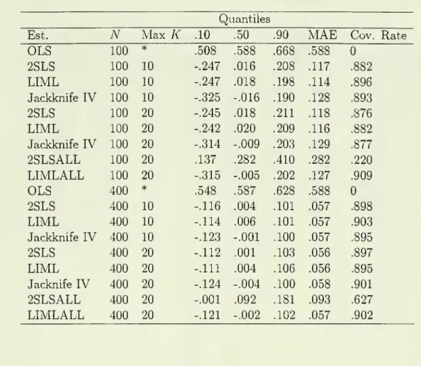
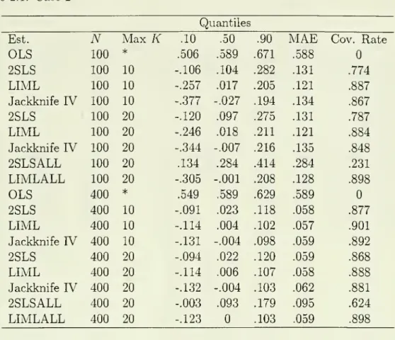
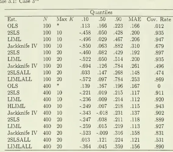
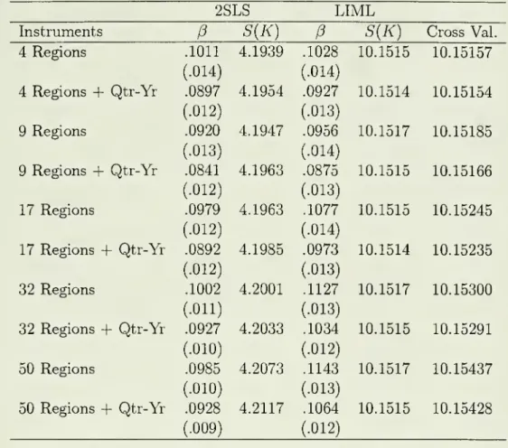
all ofthe instruments.

Tables 1.1, 2.1

and

3.1 contain the relevant

summary

statistics for each of the three cases respectively. In each table

we

report the

median

of the 5,000 estimates along with

the 0.1

and

0.9 quantiles ofthe estimates.

The

difference

between

these

can be

considered a

way

of

measuring

dispersion. Additionally

we

report the

Mean

Absolute

Error of the

estimates,

which

is

an

alternative

measure

of dispersion, and, finally, the coverage rate of a

nominal

95 percent confidence interval for each estimator. Additionally

we

report

the relevant statistics for the

OLS

estimator as well as

2SLS and

LIML

estimators that use all fc

=

20 instruments.

These

statistics were reported in

AIK

(1995, Tables 2

and

3). In Tables 1.2, 2.2

and

3.2

we

report the frequencies with

which

the various possible

K

values

were

chosen in the experiments.

A

few features ofthe results are

worth

noting. First, the

most dramatic improvements

occurinthe use of

2SLS

with theoptimal

number

ofinstrumentsbeingused.

As

indicated

in Tables 1.1

and

3.1,

2SLS

which

uses all the instruments has very

poor

properties,

and

is biased towards

OLS.

Moreover, confidence intervals generally

have

a very

poor

coverage rate with the worst occurring in

Case

1 with A'^

=

100

where

the

nominal

95%

confidence interval contains the true value just

22%

of the time.

The

other cases are similarly poor.

When

the criteria are used to choose the

number

ofinstruments there is

a substantial reduction in the bias (as

measured by

the

median)

and

the coverage rates

for the confidence intervals are

much

closer to the

nominal

rate of

_95%

generally being

around 90%.

The

only exception to this is

Case

2 with A'^

=

100

where

the coverage

rate is

below 80%,

although this is a dramatic

improvement from

the

23%

coverage rate

when

all instruments are used.

The

other noticeable difference in

2SLS

when

the criteria

is

used

is that the dispersion is

much

lower as evidenced

by reduced

MAE

and

a lower spread

between

the

10%

and

90%

quantiles. It also

worth

noting that the

performance

of

2SLS

using the criteria is not sensitive to the

maximum

K

being considered.

Indeed

the results for

2SLS

when

one uses the criteria to pick

K

with a

maximum

possible

K

of 10 are almost identical to those

when

the

maximum

possible

K

is 20.

For

LIML

on

the other hand, the

main

improvements

relative to the estimator that

by

MAE

or as the difference

between

the .1

and

.9 quantiles. This is

because

LIML

performs

fairly well

when

all of the instruments are used

and

is

approximately

median

unbiased

and

provides confidence intervals that

have

a coverage rate that is reasonably

close to the

nominal

rate of

95%

being

around 90%.

The

coverage rate for

LIML

when

the criteria is

used

is slightly lower

than

for

LIMLALL

in

Cases

1

and

2. In

Case

3,

however, there is

an

improvement

in the coverage rate

when

the criteria is

used with

the

rate being very close to the

nominal

rate.

The

main

improvement

that

comes from

the

use ofthe criteriais in the decreaseddispersion ofthe estimator

which

results in all cases.

The

performance

of

JIVE

is a little bit

mixed

relative to the other estimators.

The

bias (using the

median)

of

JIVE

in

some

cases appears to

be

the lowest

among

the

estimators

and

other cases (notably

Case

3 with 100 observations) is the worst so that

there is

no

clearly superior estimator as far as bias is concerned.

What

is striking is that the dispersion for

JIVE,

using either measure, is larger in practically all cases relative to either the

LIML

or

2SLS

estimators that result

from

the use of the criteria for picking the

number

of instruments.

There

is also

no

clear

improvement

in the coverage rates

from

the use of

JIVE

rather

than

either

2SLS

or

LIML

estimators that use the criteria for picking the

number

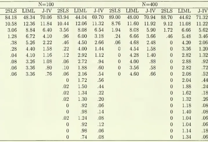
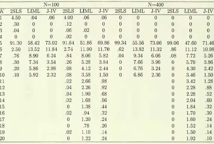
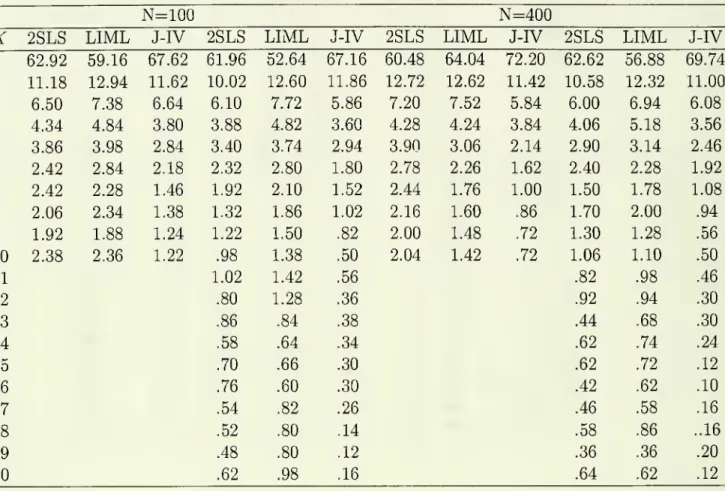
of instruments.

In Tables 1.2, 2.2

and

3.2

we

have

provided frequencies

with

which

the criteria chose the respective

number

of instruments for each estimator in each case.

A

few

features

stand

out. First, for all estimators the criteria usually points to a value of

K

that is at least as large as is required to include the relevant instrument

-

in Cases 1

and

3 this \s

K

=

\ while in

Case

2 this is /C

=

5.

What

is also interesting, is that in

Case

2 the

criteria generally pick the correct

number

ofinstriiments

more

than

halfthe time. Also,

as

one

might

expect

from

the discussioninSection 3, thecriteriafor

2SLS

generallypoints

to smaller values of

K

than

does the criteria for

JIVE,

while the latter generally picks values for

K

that are smaller (on average)

than

those for

LIML.

With

LIML

and

JIVE

the criteria

do

with

some

positive probability point to

an

instrument set that includes

many

irrelevant instruments. Fortunately, as evidenced

by

the other sets of results, this