Combinatorial aspects of total positivity

Combinatorial Aspects of Total Positivity

by

Lauren Kiyomi Williams

Bachelor of Arts, Harvard University, June 2000

Part III of the Mathematical Tripos, Cambridge University, June 2001

Submitted to the Department of Mathematics

in partial fulfillment of the requirements for the degree of

Doctor of Philosophy

at the

MASSACHUSETTS INSTITUTE OF TECHNOLOGY

June 2005

©

Lauren K. Williams, 2005. All rights reserved.

The author hereby grants to MIT permission to reproduce and

distribute publicly paper and electronic copies of this thesis document

in whole or in part.

Author.

nt of Mathematics

Certified by...

Richard P. Stanley

Norman Levinson Professor of Applied Mathematics

7

Thesis Supervisor

Accepted

by....

... .. ...

Pavel Etingof

Chairman, Department Committee on Graduate Students

MASSACHUSETTS INSTl'JTE OF TECHNOLOGY MAY 2 4 2005

LIBRARIES

j1.

..

Y.._··~~··

I: ·-

Combinatorial Aspects of Total Positivity

by

Lauren Kiyomi Williams

Submitted to the Department of Mathematics

on April 29, 2005, in partial fulfillment of the requirements for the degree of

Doctor of Philosophy

Abstract

In this thesis I study combinatorial aspects of an emerging field known as total pos-itivity. The classical theory of total positivity concerns matrices in which all minors are nonnegative. While this theory was pioneered by Gantmacher, Krein, and Schoen-berg in the 1930s, the past decade has seen a flurry of research in this area initiated by Lusztig. Motivated by surprising positivity properties of his canonical bases for

quantum groups, Lusztig extended the theory of total positivity to arbitrary reductive

groups and real flag varieties. In the first part of my thesis I study the totally non-negative part of the Grassmannian and prove an enumeration theorem for a natural cell decomposition of it. This result leads to a new q-analog of the Eulerian numbers, which interpolates between the binomial coefficients, the Eulerian numbers, and the Narayana numbers. In the second part of my thesis I introduce the totally positive

part of a tropical variety, and study this object in the case of the Grassmannian. I

conjecture a tight relation between positive tropical varieties and the cluster algebras of Fomin and Zelevinsky, proving the conjecture in the case of the Grassmannian.

The third and fourth parts of my thesis explore a notion of total positivity for

ori-ented matroids. Namely, I introduce the positive Bergman complex of an oriori-ented matroid, which is a matroidal analogue of a positive tropical variety. I prove that this object is homeomorphic to a ball, and relate it to the Las Vergnas face lattice of

an oriented matroid. When the matroid is the matroid of a Coxeter arrangement, I

relate the positive Bergman complex and the Bergman complex to the corresponding graph associahedron and the nested set complex.

Thesis Supervisor: Richard P. Stanley

Acknowledgments

I am indebted to many people for their influence on this thesis. First and foremost I would like to thank my advisor Richard Stanley, who has been a guide and inspiration in my mathematical life since I was a senior at Harvard; his insight and wisdom continually amaze me. Special thanks are due to Alex Postnikov. He suggested the problem which became Chapter 2 of this thesis, and was very generous in teaching me the necessary background for this research. In addition, I am extremely grateful to Bernd Sturmfels, who graciously agreed to advise me during the fall semester of 2003 when I was a visiting student at Berkeley. It was he who suggested the problems that became Chapters 3 and 4 of this thesis.

Many other members of the mathematical community have given me invaluable help and support. I would like to thank Sergey Fomin and Andrei Zelevinsky for stimulating discussions; their work on cluster algebras and total positivity has been an inspiration to me. In addition, I am grateful to Sara Billey, Ira Gessel, Mark Haiman, Allen Knutson, Arun Ram, Vic Reiner, Konni Rietsch, Eric Sommers, Frank Sottile, Einar Steingrimsson, and Michelle Wachs, for interesting mathematical discussions and for their encouragement of my work. Repeating names, I am grateful to Richard Stanley, Pavel Etingof, and Alex Postnikov, for agreeing to be on my thesis committee. Finally, I would like to acknowledge the math department at MIT - my fellow graduate students, the faculty, and the staff - for making the last four years such a stimulating and enriching experience for me.

I would like to thank my coauthors Federico Ardila, Carly Klivans, Vic Reiner, and David Speyer, for fruitful discussions and for their friendship. Federico and Vic hosted my visits to Microsoft Research and the University of Minnesota, respectively, where some of our work was done.

While a graduate student, I was lucky to have a fantastic community of friends in Boston (and in Berkeley). Special thanks to my friends/housemates at 516 North Street and 16 Spencer Avenue! Most of all I am grateful to Denis for his indefatigable encouragement and for making me laugh (even when not trying to).

Finally, I would like to thank my parents, John and Leila Williams, for raising me in a nurturing and stimulating environment, and my sisters Eleanor, Elizabeth, and Genevieve. They keep me on my toes and provide a constant source of amusement,

Contents

1 Introduction 13

2 Enumeration of totally positive Grassmann cells 17

2.1 Introduction ... 17

2.2 L-Diagrams ... 19

2.3 Decorated Permutations and the Cyclic Bruhat Order ... 20

2.4 The Rank Generating Function of Grk+n ... 24

2.5 A New q-Analog of the Eulerian Numbers ... .. 37

2.6 Connection with Narayana Numbers . ... . ... 42

2.7 Connections

with the Permanent ...

.. . . . .

44

3 The Tropical Totally Positive Grassmannian 45 3.1 Introduction ... ... 45

3.2 Definitions .. ... . 46

3.3 Parameterizing the totally positive Grassmannian Grk,n(R+) _{... 50}

3.4 A fan associated to the tropical positive Grassmannian ... . 57

3.5 Trop+ Gr2,n and the associahedron ... 59

3.6

Trop

+

Gr

₃

,

₆

and

the

_type

_D

₄

_{associahedron}

_{... 63}

3.7 Trop+ Gr3,7 and the type E6 associahedron ... 65

3.8 Cluster Algebras ... ... 66

4 The Positive Bergman Complex of an Oriented Matroid 73 4.1 Introduction . . . ... 73

4.2 4.3 4.4 4.5 4.6 4.7

The Oriented Matroid M, ...

The Positive Bergman Complex ...

Connection with Positive Tropical Varieties ... Topology of the Positive Bergman Complex ... The positive Bergman complex of the complete graph The number of fine cells in B3+(Kn) and B(Kn)....

5 Bergman complexes, Coxeter arrangements, graph associahedra

5.1 Introduction. ... 5.2 The matroid

MF

5.3 Graph associahedra .

5.4 The positive Bergman complex of a Coxeter arrangement ... 5.5 The Bergman complex of a Coxeter arrangement ...

A The poset of cells of Gr+,4

93 93 94 98 101 108 111 . . . .. . . . 74 . . . .... . . . 79 . . . .... . . . 83 . . . .... . . . 84 . . . .... . . . 85 . . . .... . . . 89

List of Figures

A Young diagram of shape (4,2, 1) ... A L-diagram (A, D)k ,n ...

A chord diagram for a decorated permutation ... A crossing ...

An alignment ...

Covering relation ...

Degenerate covering relations ... Recurrence for Fx(q)...

A combinatorial interpretation for yiq(T ) I.+l 1 .

A picture

of (, ) ...

...

Maximal-alignment permutations and noncrossing partitions

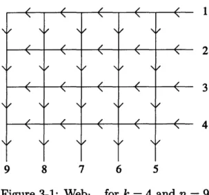
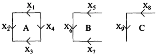
Webk,, for k = 4 and n = 9 ... Labels for regions ...

Web3,6 .

Web2,5 .

Fans for Trop Pj ... The fan of Trop+ Gr2,5 .

The intersection of F3,6 with a sphere

The intersection of F3,6 with a sphere

. . . . . . . . . . . . . . . . . . . . . . . . . . . . . . (solid torus) . . . . 4-1 The digraph D. 4-2 A point configuration ... 4-3 The digraph D'. . 2-1 2-2 2-3 2-4 2-5 2-6 2-7 2-8 2-9 2-10 2-11

... .. 19

... ..

20

... ..

21

... ..

22

... ..

22

... .. 23

... .. 24

... .. 26

... ..

35

... ..

43

... .. 50

... . .53

... ..55

... ..59

... ..60

... ..61

... ..70

... . .71

... . .75

... . .75

... ..

76

4-4 The lattice of positive flats and the lattice of flats ... 82

4-5 An equidistant tree and its corresponding distance vector. ... 85

4-6 B+(K 4) c B(K 4) . . . . . ... 88

4-7 A type r tree and an increasing binary tree of type r. ... 90

5-1 The graph-associahedron P(D4) ... .. 100

5-2 The associahedron A2 is the graph-associahedron P(A3) ... 100

5-3 The braid arrangement A3... . 105

A-1 L-diagrams ... 112

List of Tables

2.1 Ak,n(q) ... 36

2.2 Ek, (q) ... ... 39

3.1 Rays and inequalities for F3,6 ... .. . 64

Chapter 1

Introduction

In this thesis we study combinatorial aspects of an emerging field known as total positivity, as well as its relations to tropical geometry and cluster algebras. The classical theory of total positivity concerns matrices in which all minors are nonnega-tive. While this theory was pioneered by Gantmacher, Krein, and Schoenberg in the 1930s, the past decade has seen a flurry of research in this area initiated by Lusztig [30, 29, 31]. Motivated by surprising positivity properties of his canonical bases for

quantum groups, Lusztig extended the theory of total positivity by introducing the totally nonnegative variety G>o in an arbitrary reductive group G and the totally

nonnegative part B>o of a real flag variety B, which he refers to as a "miraculous polyhedral subspace" [29]. This thesis concerns combinatorial aspects of the theory of total positivity, as well as its relations to tropical geometry and cluster algebras.

Tropical algebraic geometry is the geometry of the tropical semiring (R, min, +). Its objects are polyhedral cell complexes which behave like complex algebraic varieties. Although this is a young field in which many basic questions have not yet been addressed [35], tropical geometry has already been shown to have applications to enumerative geometry, and connections to representation theory.

Cluster algebras are commutative algebras endowed with a certain combinatorial structure, which were introduced by Fomin and Zelevinsky in [21]. Though they were introduced a mere five years ago, it is already clear that cluster algebras have connections to total positivity, canonical bases, hyperbolic geometry, and quiver

rep-resentations. Remarkably, the classification of the cluster algebras of "finite type" turns out to be identical to the Cartan-Killing classification of semisimple Lie alge-bras and finite root systems [22].

This thesis is divided into four chapters, which are based on the papers [48, 41, 3, 4]. We have included a more detailed introduction at the beginning of each chapter to outline some of the background material and outline the goals of the chapter.

The first project we are concerned with is the study of the poset of cells of Post-nikov's [34] cell decomposition of the totally nonnegative part of the Grassmannian

Grk+. This poset is very interesting because it has many different combinatorial

de-scriptions, for example, in terms of certain tableaux, in terms of certain permutations, and in terms of the MacPhersonian. See Figures A-1 and A-2 for depictions of the poset of cells of Gr+ in terms of these tableaux and permutations. Our first main result is an explicit formula for the rank generating function for the poset of cells of

Grk+. One corollary of this theorem is a new proof that the Euler characteristic of Gr+n is 1. Additionally, this theorem leads to a new q-analog of the Eulerian

num-bers Ek,n(q), which specializes to the binomial coefficients, Narayana numnum-bers, and the Eulerian numbers.

Chapter 3 explores a link between totally positivity and tropical geometry.

Specif-ically, we introduce the totally positive part of the tropicalization of an arbitrary affine variety, an object which has the structure of a polyhedral fan. We then investigate

the case of the Grassmannian, denoting the resulting fan Trop+ Grk,n. We show that Trop+ Gr2,n is combinatorially the fan dual to the (type An) associahedron, and that

Trop+ Gr3,6 and Trop+ Gr3,7 are essentially the fans dual to the types D4 and E6

associahedra. These results are strikingly reminiscent of the fact that the Grassman-nian's cluster algebra structure is of types An-3, D4, and E6 for Gr2,n, Gr3,6, and Gr3,7. Finally, we conjecture a tight relation between the combinatorial structure of

a cluster algebra A and the combinatorial structure of Trop+(Spec A). This chapter is joint work with David Speyer [41].

Chapter 4 introduces a notion of total positivity for oriented matroids. Specifi-cally, the Bergman complex of a matroid is a polyhedral complex which generalizes to

matroids the notion of a tropical variety. Sturmfels introduced the Bergman complex

B(M)

of a matroid M is the order complex of the proper part of the lattice of flats LM of the matroid; this implies that B(M) is homotopy equivalent to a wedge of spheres. In this

chapter we define the positive Bergman complex B+(M) of an oriented matroid M, in order to generalize to oriented matroids the notion of the totally positive part of

a tropical variety. We also prove that, appropriately subdivided, B+_{(M) is the order} complex of the proper part of the Las Vergnas face lattice of M; it follows that B+(M)

is homeomorphic to a sphere. We conclude by showing that if M is the matroid of the complete graph, then B+(M) is dual to the face poset of the associahedron. This chapter is joint work with Federico Ardila and Carly Klivans [3].

Chapter 5 is a continuation of the work begun in Chapter 4. In this chapter we relate the positive Bergman complex and Bergman complex of (the oriented matroid

of) a Coxeter arrangement to graph associahedra and nested set complexes. Graph

associahedra are polytopes generalizing the associahedron that were independently discovered in the past year by Carr and Devadoss [10] and Postnikov [33]; these poly-topes have connections to the real moduli space of n-punctured Riemann spheres. The nested set complex of an arrangement encodes the combinatorics of its De Concini-Procesi wonderful model, as well as the combinatorics of resolutions of singularities in toric varieties. In our work we prove that the Bergman complex of a Coxeter ar-rangement A of type is equal to the nested set complex of type t, and the positive Bergman complex of A is dual to the graph associahedron of type 4. This chapter is joint work with Federico Ardila and Victor Reiner [4].

Chapter 2

Enumeration of totally positive

Grassmann cells

2.1 Introduction

The theory of total positivity dates back to the 1930s, when Gantmacher, Krein,

and Schoenberg studied matrices in which all minors are nonnegative. However, the last decade has seen a great deal of developments in this area initiated by Lusztig [30, 29, 31]. Motivated by surprising connections he discovered between his theory of canonical bases for quantum groups and the theory of total positivity, Lusztig ex-tended this subject by introducing the totally nonnegative variety G>0 in an arbitrary

reductive group G and the totally nonnegative part B>0 of a real flag variety B. A

few years later, Fomin and Zelevinsky [19] advanced the understanding of G>o by studying the decomposition of G into double Bruhat cells, and Rietsch [36] proved Lusztig's conjectural cell decomposition of B>0. Most recently, Postnikov [34] inves-tigated the combinatorics of the totally nonnegative part of a Grassmannian Grkn:

he established a relationship between Gr+ and planar oriented networks, producing a combinatorially explicit cell decomposition of Gr . In this chapter we continue Postnikov's study of the combinatorics of Gr+kn: in particular, we enumerate the cells in the cell decomposition of Grk+ according to their dimension.

]Rn is defined to be the quotient Gr+n= GL+\ Mat+(k, n), where Mat+(k, n) is the

space of real k x n-matrices of rank k with nonnegative maximal minors and GL+is the group of real matrices with positive determinant. If we specify which maximal minors are strictly positive and which are equal to zero, we obtain a cellular decomposition of

Gr+, as shown in [34]. We refer to the cells in this decomposition as totally positive cells. The set of totally positive cells naturally has the structure of a graded poset:

we say that one cell covers another if the closure of the first cell contains the second, and the rank function is the dimension of each cell.

Lusztig [30] has proved that the totally nonnegative part of the (full) flag variety is contractible, which implies the same result for any partial flag variety. (We thank

K. Rietsch for pointing this out to us.) The topology of the individual cells is not well understood, however. Postnikov [34] has conjectured that the closure of each cell in Grk* is homeomorphic to a closed ball.

In [34], Postnikov constructed many different combinatorial objects which are in one-to-one correspondence with the totally positive Grassmann cells (these objects thereby inherit the structure of a graded poset). Some of these objects include

dec-orated permutations, J-diagrams, positive oriented matroids, and move-equivalence

classes of planar oriented networks. Because it is simple to compute the rank of a

particular J-diagram or decorated permutation, we will restrict our attention to these

two classes of objects.

The main result of this chapter is an explicit formula for the rank generating

function Ak,n(q) of Grk. Specifically, Ak,n(q) is defined to be the polynomial in q whose qr coefficient is the number of totally positive cells in Grk,~ which have dimension r. As a corollary of our main result, we give a new proof that the Euler

characteristic of Grk+ is 1.

Additionally, using our result and exploiting the connection between totally pos-itive cells and permutations, we find a simple expression for a polynomial Ek,n(q)

which enumerates (regular) permutations according to weak excedences and align-ments. This polynomial Ek,n(q) is a new q-analog of the Eulerian numbers which has many interesting combinatorial properties. For example, when we evaluate Ek,n(q)

at q = -1, 0, and 1, we obtain the binomial coefficients, the Narayana numbers, and

the Eulerian numbers. Recent work of S. Corteel [13] has shown that Ek,n(q) has yet

another interpretation: it enumerates permutations according to descents and

occur-rences of the generalized pattern 13 - 2. (This result was conjectured by the author and E. Steingrimsson.) Finally, the connection with the Narayana numbers suggests a way of incorporating noncrossing partitions into a larger family of "crossing"

par-titions.

Let us fix some notation. Throughout this chapter we use [i] to denote the q-analog of i, that is, [i] = 1 + q + + qi-1. (We will sometimes use [n] to refer to the set {1,..., n}, but the context should make our meaning clear.) Additionally,

[i]! := rn=_ [k] and _k-i

[: - -

_[iUj

2.2 J-Diagrams

A partition A = (Al, ... , Ak) is a weakly decreasing sequence of nonnegative numbers.

For a partition A, where E Ai = n, the Young diagram Yx of shape A is a left-justified

diagram of n boxes, with Ai boxes in the ith row. Figure 2-1 shows a Young diagram of shape (4, 2, 1).

Figure 2-1: A Young diagram of shape (4,2, 1)

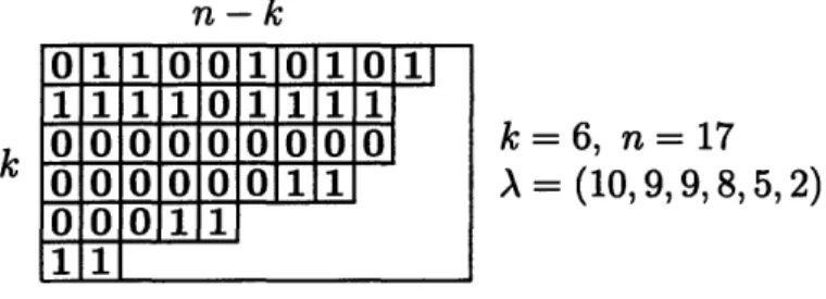
Fix k and n. Then a J-diagram (A, D)k,n is a partition A contained in a k x (n - k)

rectangle (which we will denote by (n - k)k), together with a filling D: Yx - (0, 1} which has the J-property: there is no 0 which has a 1 above it and a 1 to its left. (Here, "above" means above and in the same column, and "to its left" means to the left and in the same row.) In Figure 2-2 we give an example of a J-diagram. 1

1_{The symbol J is meant to remind the reader of the shape of the forbidden pattern, and should}

be pronounced as [le], because of its relationship to the letter L. See [34] for some interesting numerological remarks on this symbol.

n-k

11zolllllfl

k

6, n=17

A= (10, 9,9,8,5,2)

Figure 2-2: A J-diagram (A, D)k,n

We define the rank of (A, D)k,n to be the number of 's in the filling D. Postnikov proved that there is a one-to-one correspondence between J-diagrams (A, D) contained in (n - k)k, and totally positive cells in Gr+n, such that the dimension of a totally positive cell is equal to the rank of the corresponding J-diagram. He proved this by providing a modified Gram-Schmidt algorithm A, which has the property that it maps a real k x n matrix of rank k with nonnegative maximal minors to another matrix whose entries are all positive or 0, which has the 1-property. In brief, the bijection between totally positive cells and J-diagrams maps a matrix M (representing some totally positive cell) to a J-diagram whose 's represent the positive entries of A(M). Figure A-1 shows the poset of cells of Gr+4 in terms of J-diagrams.

Because of the correspondence between cells and J-diagrams, in order to compute

Ak,n(q), we need to enumerate J-diagrams contained in (n - k)k according to their number of l's.

2.3 Decorated Permutations and the Cyclic Bruhat

Order

The poset of decorated permutations (also called the cyclic Bruhat order) was intro-duced by Postnikov in [34]. A decorated permutation r = (7r, d) is a permutation r in the symmetric group

Sn

r(i) = i by two colors. Usually we refer to these two colors as "clockwise" and

"counterclockwise," for reasons which the next paragraph will make clear.

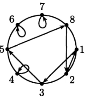
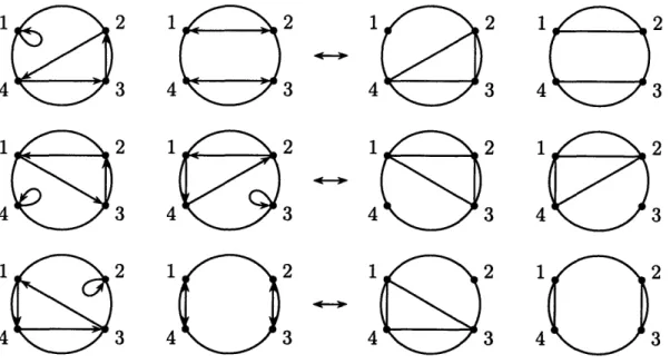
We represent a decorated permutation ir = (r, D), where r E S,, by its chord

diagram, constructed as follows. Put n equally spaced points around a circle, and 20

label these points from 1 to n in clockwise order. If r(i) = j then this is represented as a directed arrow, or chord, from i to j. If 7r(i) = i then we draw a chord from i to i (i.e. a loop), and orient it either clockwise or counterclockwise, according to d. We refer to the chord which begins at position i as Chord(i), and we use ij to denote

the directed chord from i to j. Also, if i, j E {1,..., n}, we use Arc(i, j) to denote the set of points that we would encounter if we were to travel clockwise from i to j,

including

i and j.

For example, the decorated permutation (3, 1, 5, 4, 8, 6, 7, 2) (written in list nota-tion) with the fixed points 4, 6, and 7 colored in counterclockwise, clockwise, and counterclockwise, respectively, is represented by the chord diagram in Figure 2-3.

7

1

3

Figure 2-3: A chord diagram for a decorated permutation

The symmetric group

Sn acts on the permutations in

Sn by conjugation. This

Sn

We say that a pair of chords in a chord diagram forms a crossing if they intersect inside the circle or on its boundary.

Every crossing looks like Figure 2-4, where the point A may coincide with the

point B, and the point C may coincide with the point D. A crossing is called a simple crossing if there are no other chords that go from Arc(C, A) to Arc(B, D).

Say that two chords are crossing if they form a crossing.

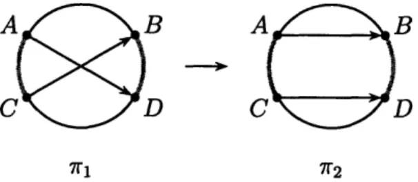
Let us also say that a pair of chords in a chord diagram forms an alignment if they are not crossing and they are relatively located as in Figure 2-5. Here, again, the

C

Figure 2-4: A crossing

A

B

C

D

Figure 2-5: An alignment

point A may coincide with the point B, and the point C may coincide with the point D. If A coincides with B then the chord from A to B should be a counterclockwise

loop in order to be considered an alignment with Chord(C). (Imagine what would happen if we had a piece of string pointing from A to B, and then we moved the

point B to A). And if C coincides with D then the chord from C to D should be a

clockwise loop in order to be considered an alignment with Chord(A). As before, an alignment is a simple alignment if there are no other chords that go from Arc(C, A) to Arc(B, D). We say that two chords are aligned if they form an alignment.

We now define a partial order on the set of decorated permutations. For two decorated permutations 7r1 and r2of the same size n, we say that 7rl covers r2, and

write rl --, r2, if the chord diagram of r contains a pair of chords that forms a

simple crossing and the chord diagram of 7r2 is obtained by changing them to the

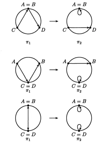
pair of chords that forms a simple alignment (see Figure 2-6). If the points A and B happen to coincide then the chord from A to B in the chord diagram of 7r2 degenerates to a counterclockwise loop. And if the points C and D coincide then the chord from

C to D in the chord diagram of 7r2 becomes a clockwise loop. These degenerate situations are illustrated in Figure 2-7.

A%

J

B

C

ZD

7r1 72

Figure 2-6: Covering relation

Let us define two statistics A and K on decorated permutations. For a decorated permutation r, the numbers A(7r) and K(7r) are given by

A(7r) = #{pairs of chords forming an alignment},

K(7r) = #{i I 7r(i) > i} + #{counterclockwise loops}.

In our previous example r = (3, 1, 5, 4, 8, 6, 7, 2) we have A = 11 and K = 5. The 11 alignments in 7r are (13,66), (21,35), (21,58), (21,44), (21, 77), (35,44), (35,66),

(44, 66), (58, 77), (66, 77), (66, 82).

Lemma 2.3.1.

[34]

then

and K(7rl)

Lemma 2.3.1 implies that the transitive closure of the covering relation "-" has

the structure of a partially ordered set and this partially ordered set decomposes into n + 1 incomparable components. For 0 < k < n, we define the cyclic Bruhat order

CBkn as the set of all decorated permutations r of size n such that K(lr) = k with

the partial order relation obtained by the transitive closure of the covering relation

"--". By Lemma 2.3.1 the function A is the corank function for the cyclic Bruhat order CBkn.

The definitions of the covering relation and of the statistic A will not change if we rotate a chord diagram. The definition of K depends on the order of the boundary

A=B

A=B

C=D

D

A=B

CUD

B

A=B

C=D

Figure 2-7: Degenerate covering relations

cyclic shift conj, for the long cycle = (1, 2,..., n). Thus the order CBkn is invariant under the action of the cyclic group Z/nZ on decorated permutations.

In [34], Postnikov proved that the number of totally positive cells in Gr+,n of dimension r is equal to the number of decorated permutations in CBkn of rank r. Thus, Ak,n(1) is the cardinality of CBkn, and the coefficient of qk(n-k)-t in Ak,n(q) is the number of decorated permutations in CBkn with e alignments.

Figure A-2 shows the poset of cells of Grj 4 in terms of decorated permutations.

2.4 The Rank Generating Function of Grk

Recall that the coefficient of qr in Ak,n(q) is the number of cells of dimension r in the cellular decomposition of Grk . In this section we use the J-diagrams to find an

ex-plicit expression for Ak,n(q). Additionally, we will find exex-plicit expressions for the

gen-erating functions Ak(q, x) := an Ak,n(q)xn and A(q, x, y) := k>l n Ak,n(q)Xnyk.

Our main theorem is the following:

Theorem 2.4.1.

-y

A(q,

+ l yi(q 2i+l _Y)

l qi2+l (qi-q[[i + 1]x +[i]xy)

Ak

(q,

x)

+

i=o Ak(qki+i+l(l

-

[i +

l]x)k

_i

₍₁₎

_qki(l

_{[ + ]x)k-il}

k-1

k- ()q ([ +

k +

Note that it is not obvious from the above formulas that Ak,n(q) is either polyno-mial or nonnegative.

Since the expressions for Ak(q, x) and Ak,n(q) follow easily from the formula for

A(q, x, y), we will concentrate on proving the formula for A(q, x, y).

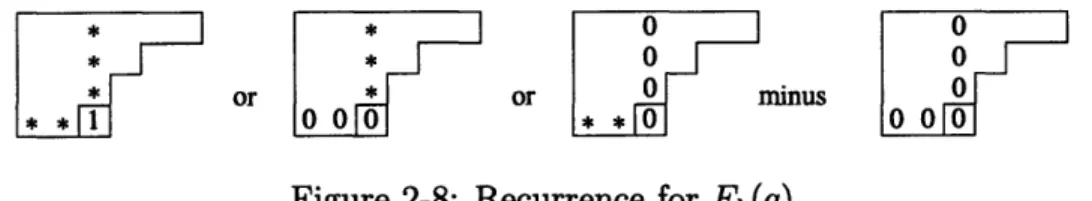
Fix a partition A = (Al,... ., k). Let F,(q) be the polynomial in q such that the coefficient of qr is the number of -fillings of the Young diagram Yx which contain r

l's. As Figure 2-8 illustrates, there is a simple recurrence for FA(q).

Explicitly, any l-filling of A is obtained in one of the following ways: adding a 1 to the last row of a -filling of (Al, 2, ... , Ik-1, Ak- 1); adding a row containing Ak O's to a J-filling of (Al, . , Ak-1); or inserting an all-zero column after the (Ak - )st

column of a 1-filling of (Al - 1, A2 - 1,...,Ak - 1). Note, however, that the second and third cases are not exclusive, so that our resulting recurrence must subtract off

a term corresponding to their overlap.

Remark 2.4.2.

Fx(q) qF(x ...k-,Xk-l)(q) + F(X1 ... k-l)(q) + F(AI-l,...,Ak-l)(q) - F(x,-l...,...kl-l)(q) 25

0 0

*

_*

_]0

0

· * *I0

**0

0 0

Figure 2-8: Recurrence for FA(q)

From the definition, or using the recurrence, it is easy to compute the first few formulas. Here are F(Ax)(q) and F(l,x,)(q).

Proposition 2.4.3.

F(\)(q) = [2]

_\

F(A, 2) (q) = -q-[2]1 + q-1[2]A-2+1[ 3]A2

In general, we have the following formula.

Theorem 2.4.4. Fix A = (A1, A2, ., Ak). Then

k i

F (q)

y

-Atj+1

i=l l=t <...<ti<k j=2

where M(tl,..., ti

:

k) = (l)k+iq-ik+Ejltj [i]k-ti nJ-,;ltj+-tj-1

Before beginning the proof of the theorem, we state two lemmas which follow immediately from the formula for M(tl,..., ti : k).

Lemma 2.4.5. M(tl,...,

ti

k) = (-l)k-tiq-i(k-ti)[i]k-tiM(tl,..., t : t).

Lemma 2.4.6.

M(tl,...,ti:

ti) =

-[i

1]-M(tl,...,ti-1:

ti).

Proof. To prove the theorem, we must show that the expression for Fx(q) holds for

A = (A1), and that it satisfies the recurrence of Remark 2.4.2. Also, we must show

that F(xX1 \2,...,Ak)(q) = F(A1,X2,..k,)(q )

The formula F(A) (q) = [2]X1 clearly agrees with the expression in the theorem. To

show that the recurrence is satisfied, we will fix (tl,..., ti) where 1 = tl < -. < ti < k,

and calculate the coefficient of [2]Atl-\t2+1[3]At2-t 3+1 ... [i + 1]Ati in each of the five

terms of 2.4.2. We will then show that these coefficients satisfy the recurrence.

The coefficient in F(Axl...,k)(q) is M(tl,..., ti : k).

The coefficient in F(xl,xA2... xk-1)(q) is M(t,..., ti : k) if ti < k, because the term

we are looking at together with its coefficient do not involve Ak. The coefficient is

[i][i + l]-'M(tl,..., ti,: k) if ti = k.

The coefficient in F(XlA2 .X k-l)(q) is M(tl,... .. , ti: k - 1) if ti < k, which is equal

to -qi[i]-lM(tl,... ,ti: k). But if ti = k, no such term appears, so the coefficient is 0.

The coefficient in F(xA-l,A2-1,...Ak-1)(q) is always M(tl,..., ti : k)[i + 1]- 1_.

The coefficient in F(A1-1,2-1,. ..,_-l-1)(q) is -qi[i]-l[i + ]-1M(tl,... ,ti : k) if ti < k, and 0 if ti = k.

Let us abbreviate M(tl,..., ti : k) by M. We need to show that the coefficients we

have just calculated satisfy the recurrence of Remark 2.4.2. For ti < k, this amounts

to showing that M = qM - qi[i]-lM + M[i + 1]-1 + qi[i]-l[i + 1]-1M. And for ti = k, we must show that M = q[i][i + 1]-1M + M[i + 1]-1. Both of these are easily seen to

be true. Thus, we have shown that our expression for Fx(q) satisfies Remark 2.4.2.

Now we will show that F(A1,x2,...,xkl,o)(q) = F(A1,A2,...,xk 1)(q). It is sufficient to show

that the coefficient of [2]At-At2+l[3]Xt2-At3+1 ... [i + 1]Ati in F(l,...,Ak)(q), plus [i + 1]

times the coefficient of [2]tl-Xt 2+l[3]Xt2-t 3+1 ... [i + 1]ti-Ak+1 [i + 2]k in F(Al,...,k)(q),

is equal to the coefficient of [2]Xtl-t2+1 .. . [i + 1]Xti in F(x1...,xAk_)(q).

In other words, we need

M(tl,...

,ti:

k- 1) = M(tl,...,ti: k) + M(tl,...,ti, k: k)[i + 1].

From the formula for M, we have M(tl,...,ti : k - 1) = -qi[i]-l1M(tl,..., ti : k).

And from Lemma 2.4.6, M(tl,...,t i, k: k) = -[i]-lM(tl,...,ti : k). The proof

follows.

[

Recall that Ak(q, x) is the polynomial in q and x such that [qxn]Ak(q, x) is equal to the number of totally positive cells of dimension r in Gr+n. This is equal to the number of J-diagrams (A, D)k,n of rank r. We can compute these numbers by using Theorem 2.4.4.

Corollary 2.4.7.

k i)k+iq_/+Ej'lt tj+l-tj

Ak(q,

=

E E

(-)k+q

1

j1]

i=1 =t<...<t+=k+l (1 - x) 1 + 1X

To compute Ak(q, x), we must sum F(Ax,...,xk)(q)xn, as A varies over all partitions which fit into a k x (n - k) rectangle. To do this, we use the following simple lemmas,

the second of which follows immediately from the first.

Lemma 2.4.8.

00 ,1 Ad-1

E

XX2

A1=0A2=0 ,d=O

Lemma 2.4.9. Fix a set of positive integers tl < t t2 < .. < td < n + 1. Then

o0 n A 1 Ad-1

E E E

...

E

n=O A1=0 A2=O Ad=O

is equal to

(1 - x)(1 - [2]x)t2-tl ... (1 - [d]x)td-td-1 (1 - [d + 1]X)n+l -_td'

Proof. For the proof of the corollary, apply Theorem 2.4.4 and Lemma 2.4.9 to the fact that

oo m A1 Ak-1

Ak(q,x) = E E

F, ..,n,)

m=0 A1=0 A2=0 Ak=O

Corollary 2.4.10. The Euler characteristic of the totally non-negative part of the

Grassmannian Grkn is 1.

Proof. Recall that the Euler characteristic of a cell complex is defined to be i (- )ifi, where fi is the number of cells of dimension i. So if we set q = -1 in Corollary 2.4.7, we will obtain a polynomial in x such that the coefficient of xn is the Euler characteristic of Grk , . Notice that [i] is equal to 0 if i is even, and 1 if i is odd.

So all terms of Ak(-l, x) vanish except the term for i = 1, which becomes 1 =

Xk + xk+1 + Xk+2 _{+ ....}

Note that this corollary also follows from Lusztig's result that the totally nonneg-ative part of a real flag variety is contractible.

Now our goal will be to simplify our expressions. To do so, it is helpful to work

with the "master" generating function A(q, x, y) := Ek>1 Ak(q, x)yk. As a first step,

we compute the following expression for A(q, x, y):

Proposition 2.4.11.

00 1

A(q, x, y)

=

q[i]!x'

Yi

qj+]

+ ]xy

Note that _{qJ-qJ[ j+]x+[j]xy}1 is not a well-defined formal power series because it is not clear how to expand it. In this chapter, for reasons which will become clear in the following proof, we shall always use 1 as shorthand for the formal power series whose expansion is implied by the expression

1

qj(1 -

[+

1]x)(1

See [43, Example 6.3.4] for remarks on the subtleties of such power series.

Proof. From Corollary 2.4.7, we know that Ak(q, x) is equal to

(-Z)k

-ik+j

j

a]

+

),

i=1 l=tl<<ti+lk+l j1

1

x

If we make the substitution aj = tj+l - tj, we then get

Ak(q,x) (-

z

(1

ajl =kj---

is equal to _{q3-q3[j+l]x-[jjy} - ]- ]y- We get_ege

Ak(q,x) =

_{(- "-] 1),q}

_{1-x .}

i=1

i

aj>l j=l

and we can now easily compute A(q, x, y) := Ek>l Ak(q, X)Yk.

A(q, , y) =

_1-x

E(-X)kE(-l)iq

i

fI fj(aj)y"i

j=l

i

E

(-x)k(-1)qi

H

fj(aj)Y'i

Actually, we can replace k > i above with k > 0, since if k < i there will be no set of

aj satisfying the conditions of the third sum. So we have

1 00

A(q, x, y)= r

E

1-x

E

i=E(-l)i

1-x

'IJ

fi(aj)yi

E

II fJ(aj)(-xY)'J

- 1)'q'H Fj (-xy

E(- 1)q

i

j

ja;y

~-

qt[i]!xiy

ij

qi-qIj + l]x

+ ]xy

qj -q[j q

+

1]x +

j]xy

q - q + 1]x + [j]xy'

=1

_ E qi[i]!xiyi

=

i=1 k>i arj>l al+--+ai=k

.

Now we will prove the following identity. This identity combined with Proposition 2.4.11 will complete the proof of Theorem 2.4.1.

Theorem 2.4.12.

0q[]!0t7J1-

q -i

_-i-lyi(q2i+l

2

_-

_y)

i=

q -q'

Ij+ ]x

+ ]xy

-

E qi _qi

+]x++

[i]xy

Proof. Observe that the expression on the right-hand side can be thought of as a

partial fraction expansion in terms of x, since all denominators are distinct, and

the numerators are free of x. Also note that the i-summand of the left-hand side

should be easy to express in partial fractions with respect to x, since all factors of

the denominator are distinct and the x-degree of the numerator is smaller than the

x-degree of the denominator.

Thus, our strategy will be to put the left-hand side into partial fractions with

respect to x, and then show that this agrees with the right-hand side.

To this end, define ,i(j) by the equation

xi i /i(j)

nI=

i i

X

E

/3,(j)

qr[r +

1]x

+

[r]xy).

(2.1)

j=O r=O

rTj

Fix

j.

Notice that (qi

-

q[j + 1]x + [j]xy) vanishes

when x = -i----

SO

substitute x = qj into (2.1). We get

fqij

)

(qj[j + 1]- [j]y)i r=O qj[j + 1]- [j]y

Solving for 3i(j) and simplifying, we arrive at

A(j) =

_ q-r-j-ly)

Thus the partial fraction expansion with respect to x of the left-hand side of Theorem 2.4.12 is 00 i /i(j)qi[i]!y i =E

E

j]xy'

E

[,] q-('+2)-i (-y)i

(1

qi - qj + 1]x

+

[j]xy

Now it remains to show that the numerator of (qj - q[j + 1]x + [j]xy) in (2.2) is equal to the numerator of (qJ - qJ[j + 1]x + [j]xy) in the right-hand side of Theorem 2.4.12. For j = 0, we must show that

(1 - ) ( q i> i

-1)iq-(i+l)y

fI(l

_ q-r-l1)-1 = -y

And for j > 0, we must show that

i

(-_l)jq 3

J

E

_[;]

q(i+')-'ij(y)i

_q-r-j-ly)-1

_1.

i>

_ilj

j

r=O

(2.4)

If we make the substitution q -- q-l1 and r - r - 1 into (2.3) and then add the

i = 0 term to both sides, we obtain

(-1)iyiq(i+) i>O i+1 .l 1 - qry r=1 (2.5) _ q-r-j-ly)-1 (2.2)

And if we make the same substitution into (2.4), we get

i+1

(-iq()y-i

E(_l),q(i+l);]II

rT =

1.

(2.6)

i>j r=l

Since (2.5) is a special case of (2.6), it suffices to prove (2.6). We will prove this

as a separate lemma below; modulo this lemma, we are done. O

Lemma 2.4.13.

(-l)q -(j+2)y-

i(

=j

Proof. Christian Krattenthaler has pointed out to us that this lemma is actually a special case of the 1l summation described in Appendix II.5 of [24]. Here, we give two additional proofs of this lemma. The first method is to show that the infinite sum actually telescopes (we thank Ira Gessel for suggesting this to us). The second

method is to interpret the lemma as a statement about partitions, and to prove it

combinatorially.

Let us sketch the first method. We use induction to show that

j+ m-1 i+1 (-l) q(') ]yi +j i=j

[

]r=l

j

fl

Then we take the limit as m goes to oo, obtaining the statement of the lemma. Now let us give a combinatorial proof of the lemma. For clarity, we prove the

j = 0 case in detail and then explain how to generalize this proof.

First we claim that (-l)iy'q(+l1) .+- l['1y is a generating function for partitions

A with i + 1 parts, all distinct, where the smallest part may be zero. In this formal power series, the coefficient of ym"q is equal to the number of such partitions with

m columns and n total boxes. The generating function is multiplied by 1 or -1,

according to the parity of the number of rows (including zero).

To prove the claim, note that each term of rj+l

1

boxes. Now take the transpose of this partition, so that it is a partition with exactly i + 1 rows (possibly zero). Now the exponent of y is the length of the longest row.

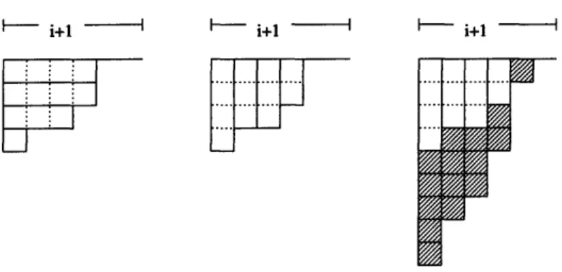
Add i, i- 1,..., 1 and 0 boxes to the first, second, ... , and (i+ 1)st rows, respectively. Finally we have a partition with i+1 parts, all distinct, where the smallest part may be zero. Since we've added a total of (i+1) boxes to the original partition, the generating function for this type of partition is q( 2 )yi tij Figure 2-9 illustrates the steps in this paragraph. In the figure, the rows and columns of the partitions are indicated by solid and dashed lines, respectively.

i+l I i+lI I i+l i+lI

Figure 2-9: A combinatorial interpretation for y'q( 2 ) ni+l 1ry

Now we need to find an involution 0 which explains why all of the terms on the left-hand side of (2.5) cancel out, except for the 1. This involution is very simple:

if (A1,...,Ak) is a partition such that Ak

#

0)-And if Ak = 0, then (A, ... , Ak) = (A, ... ,Ak-l). Clearly both (Al,...,Ak) and O(A1,... , Ak) contribute the same powers of y and q to the generating function; the

only difference is the sign. Only the 0 partition has no partner under the involution,

so all terms cancel except for 1.

. . .

_ _ : : ... - . . : .. ...

-For the proof of the general case, we will show that

q(i+l)[;]i-j (2.7)

qQ

)[yifJ

i a

1

g

enumerates certain pairs of partitions, (A, A). First, note that _r=1 +1 _1+y 1 _is is a gen-_a

gen-erating function for partitions with rows of lengths j + 1 through i + j + 1, inclusive.

It is well-known that

]

underneath a partition with rows of lengths j + 1 through i + j + 1, giving us a

par-tition with row lengths between 0 and i + j + 1, inclusive. We consider this parpar-tition to have exactly i + j + 1 columns, possibly zero. Finally, to account for the q(T+)

term in (2.7) let us add 0, 1,..., i boxes to the last i + 1 columns of our partition, so

that that the last i + 1 columns have distinct lengths (possibly zero). We now view the boxes in the first j columns of our figure to comprise one partition A, and the boxes in the last i + 1 columns of our figure to comprise the transpose of a second partition A. Let Al denote the length of the first row of A, and let rj(A) denote the number of rows of A which have length j. Then the pair (A, A) satisfies the following conditions: A has rows with lengths between 0 and j, inclusive; A has exactly i + 1 rows, all distinct, where the smallest row can have length 0; and rj(A) + i -j = l.

(See Figure 2-10 for an illustration of (A, A).) The term in (2.7) that corresponds to this pair of partitions is qll+llynumparts(A).

; . ;l .:,

T i-j

1

Our involution 0 is a simple generalization of the involution we used before. This time, fixes A, and either adds or subtracts a trailing zero to A.

This completes the proof of Theorem 2.4.1.

Remark 2.4.14. Discovering the formulas which appear in Theorem 2.4.1 was

non-trivial. In our early work on this subject, we were able to compute by hand closed expressions for A (q, x), A2(q, x), A3(q, x), and A4(q, x). By looking at the partial fraction expansion of these expressions we were able to see enough patterns to

conjec-ture the formula for Ak(q, x) in Theorem 2.4.1.

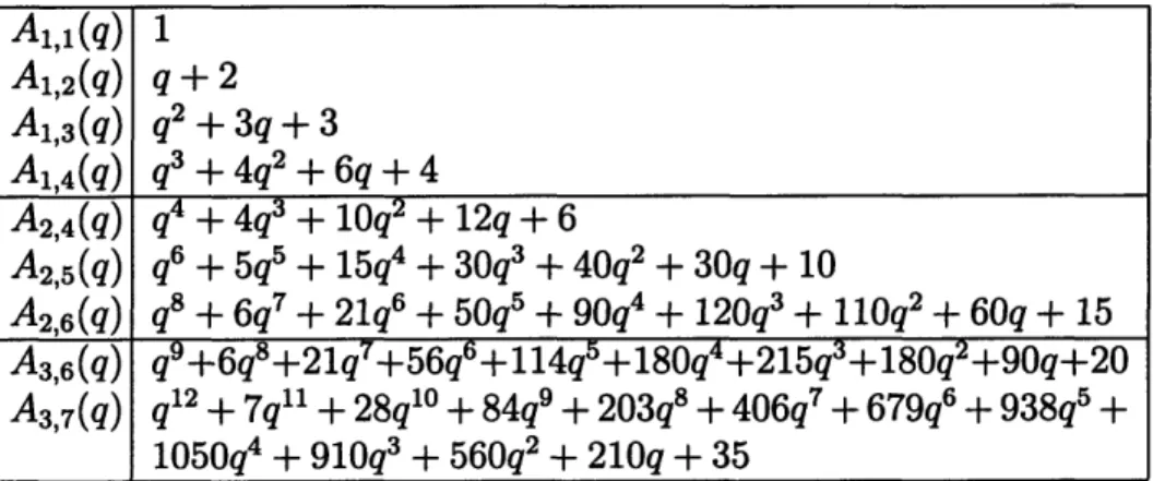
In Table 2.1, we have listed some of the values of Ak,n(q) for small k and n. It is easy to see from the definition of J-diagrams that Ak,n(q) = An-k,n(q): one can

reflect a diagram (A, D)k,n of rank r over the main diagonal to get another J-diagram (A', D')n-k,n of rank r. Alternatively, one should be able to prove the claim directly from the expression in Theorem 2.4.1, using some q-analog of Abel's identity.

Table 2.1: Ak,n(q)

Note that it is possible to see directly from the definition that Grt+ is just some deformation of a simplex with n vertices. This explains the simple form of Al,n(q).

A1,l(q) 1 A1,2(q) q +2 A1,3(q) q2 + 3q + 3 A1,4(q) q3+ 4q2+ 6q

+ 4

2.5 A New q-Analog of the Eulerian Numbers

If 7r E Sn, we say that 7r has a weak excedence at position i if r(i) > i. The Eulerian

number Ek,n is the number of permutations in S, which have k weak excedences.

(One can define the Eulerian numbers in terms of other statistics, such as descent, but this will not concern us here.)

Now that we have computed the rank generating function for CBk+ (which is the rank generating function for the poset of decorated permutations), we can use this result to enumerate (regular) permutations according to two statistics: weak excedences and alignments. This gives us a new q-analog of the Eulerian numbers.

Recall that the statistic K on decorated permutations was defined as

K(7r) = #{i 1 7r(i) > i + #{counterclockwise loops}.

Note that K is related to the notion of weak excedence in permutations. In fact, we can extend the definition of weak excedence to decorated permutations by saying that a decorated permutation has a weak excedence in position i, if 7r(i) > i, or if r(i) = i

and d(i) is counterclockwise. This makes sense, since the limit of a chord from 1 to 2 as 1 approaches 2, is a counterclockwise loop. Then K(7r) is the number of weak excedences in 7r.

We will call a decorated permutation regular if all of its fixed points are oriented counterclockwise. Thus, a fixed point of a regular permutation will always be a weak excedence, as it should be. Recall that the Eulerian number Ek,n is the number of permutations of [n] with k weak excedences. Earlier, we saw that the coefficient of

qk(n-k)-t in Ak,n(q) is the number of decorated permutations in CBkn with

e

align-ments. By analogy, let Ek,n(q) be the polynomial in q whose coefficient of qk(n-k)-t is the number of (regular) permutations with k weak excedences and

e

We can relate decorated permutations to regular permutations via the following lemma.

Lemma 2.5.1. Ak,n(q) = EZin ()Ek,n-i(q).

Proof. To prove this lemma we need to figure out how the number of alignments

changes, if we start with a regular permutation on [n - i] with k weak excedences, and then add i clockwise fixed points. Note that adding a clockwise fixed point adds exactly k alignments, since a clockwise fixed point is aligned with all of the weak excedences. Since clockwise fixed points are not in alignment with each other, it follows that adding i clockwise fixed points adds exactly ik alignments.

This shows that the new number of alignments is equal to ki plus the old number of alignments, or equivalently, that k(n - i - k) minus the old number of alignments is equal to k(n - k) minus the new number of alignments. In other words, the rank of the permutation on [n - i] is equal to the rank of the new decorated permutation on [n]. Both permutations have k weak excedences. Since there are () ways to pick

i entries of a permutation on [n] to be designated as clockwise fixed points, we have that Ak,n(q) =

Ein

Observe that we can invert the formula given in the lemma, deriving the following corollary.

Corollary 2.5.2.

Ek,n(q) = E(-1)i Aki,,,(q).

Putting this together with Theorem 2.4.1, we get the following.

Corollary 2.5.3.

k-1

Ek,(q)

=

qn-k

Z

(-n)

_{(1)i(qki-[k-i]}

_{q[k -i-1]}

k-1

= q-k 2

Z()i[k

_]nqki-k(

₊

(i

)

Notice that by substituting q = 1 into the second formula, we get

Ek,

=

i(_)i(n+

l)(k

-

i)n

the well-known exact formula for the Eulerian numbers.

Now we will investigate the properties of Ek,n(q). Actually, since Ek,n(q) is a multiple of qn-k, we first define E,n(q) to be qk-nEk,n(q), and then work with this renormalized polynomial. Table 2.2 lists Ek,n(q) for n = 4, 5,6, 7.

Table 2.2: k,n(q)

We can make a number of observations about these polynomials. For example, we

can generalize the well-known result that Ek, = En+l-k,n, where Ek,n is the Eulerian E1,₄(q) 1 E2,4(q) 6 + 4q + q2 /3,4(q) 6 + 4q + q2 E₄,₄(q) 1 E1,5(q) 1 E2,5(q) 10 + 10q + 5q2 + q3 E3,5(q) 20 + 25q + 15q2 + 5q3 + q4 E4,5(q) 10 + 10q + 5q2 + q3 E₅,₅(q) 1 E1,6(q) 1 E2,6(q) 15 + 20q + 15q2 + 6q3 + q4 E3,6(q) 50 + 90q + 84q2 + 50q3 + 21q4 + 6q5 + q6 E4,6(q) 50 + 90q + 84q2 + 50q3 + 21q4 + 6q5 + q6 5 ,6(q) 15 + 20q + 15q2+ 6q3 + q4 E6,6(q) 1 El,7(q) 1 E2,7(q) 21 + 35q + 35q2 + 21q3 + 7q4 + q5 E3,7(q) 105+ 245q+ 308q2+ 259q3+ 161q4+ 77q5+ 28q6 + 7q7 + q8 E4,7(q) 175 + 441q + 588q2 + 532q3 + 364q4 + 196q5 + 84q6 + 28q7 + 7q8 + q9 E5,7(q) 105+245q+308q 2+ 259q3+ 161q4+ 77q5 + 28q6+ 7q7+q8 E6,7(q) 21 + 35q + 35q2 + 21q3 + 7q4 + q5 E7,7(q) 1

number corresponding to the number of permutations of S, with k weak excedences.

Proposition

2.5.4.

Proof. To prove this, we define an alignment-preserving bijection on the set of permu-tations in Sn, which maps permupermu-tations with k weak excedences to permupermu-tations with n+1-k weak excedences. If 7r = (al, a2,..., an) is a permutation written in list

nota-tion, then the bijection maps r to (bl, b2, .. , b), where bi = n-an+li modulon.

The reader will probably have noticed from the table that the coefficients of 2,n (q)

are binomial coefficients. Indeed, we have the following proposition, which follows from Corollary 2.5.3.

Proposition 2.5.5. E2,n(q) = i=O (i+2)qi.

Proposition 2.5.6. [34] The coefficient of the highest degree term of Ek,n(q) is 1.

Proof. This is because there is a unique permutation in Sn with k weak excedences

and no alignments, as proved in [34]. That unique permutation is rk : i i +

k modulo n. U

Proposition 2.5.7. Ek,n(-1) = k-1)

Proof. If we substitute q = -1 into the first expression for Ek,n(q), we eventually get

(-)n+l

ELk-

Proposition 2.5.8. Ek,n(q) is a polynomial of degree (k - 1)(n - k), and Ek,n(O) is

the Narayana number Nk,n = n (k) (k l)

We will prove Proposition 2.5.8 in Section 2.6.

Corollary 2.5.9. Ek,n(q) interpolates between the Eulerian numbers, the Narayana

numbers, and the binomial coefficients, at q = 1, 0, and -1, respectively.

Proof. This follows from the fact that Ek,n(q) is a q-analog of the Eulerian numbers,

Based on experimental evidence, we formulated the following conjecture about the coefficient of q in /k,n(q). However, nice expressions for coefficients of other terms have eluded us so far.

Conjecture 2.5.10. The coefficient of q in

Ek,n(q)

Remark 2.5.11. The coefficients of Ek,n(q) appear to be unimodal. However, these

polynomials do not in general have real zeroes.

Since it may be helpful to have formulas which enumerate permutations by align-ments (rather than k(n - k) minus the number of alignalign-ments), we let Ek,n(q) be the polynomial in q such that the coefficient of q' is the number of permutations on {1,... n} with k weak excedences and 1 alignments. Note that by using Corollary 2.5.3 and performing a transformation which sends q to q-1, we get the following expressions. k-1

Ek,n(q) = E

(

(-1)iqi(n-k)(q[k - i]

_{- qn[k - i - 1]}

₎

=

Z(-l)i[k

i]nqi(n-k)(nqi+

n )qk)

Remark 2.5.12. An occurrence of the generalized pattern 13- 2 in a permutation r

is a triple of indices (i, i + 1, j) where i + 1 < j such that ri < 7rj < 7ri+l. Together with E. Steingrimsson [45], we conjectured that the polynomials tk,n(q) enumerated permutations according to descents and occurrences of the generalized pattern p, where

p is any one of the patterns 13 - 2, 31 - 2, 2 - 13, 2 - 31. This conjecture was subse-quently proved by Sylvie Corteel [13]. Additionally, she showed that the polynomials

Ek,n(q) arise in the study of the ASEP model in statistical physics [13].

Theorem 2.5.13. [13] The coefficient of qT in Ek,n(q) is the number of permutations on n letters with k - 1 descents and r occurrences of the generalized pattern 13 - 2.

2.6 Connection with Narayana Numbers

A noncrossing partition of the set [n] is a partition r of the set [n] with the property

that if a < b < c < d and some block B of r contains both a and c, while some block B' of 7r contains both b and d, then B = B'. Graphically, we can represent a noncrossing partition on a circle which has n labeled points equally spaced around it. We represent each block B as the polygon whose vertices are the elements of B. Then the condition that r is noncrossing just means that no two blocks (polygons) intersect each other.

It is known that the number of noncrossing partitions of [n] which have k blocks is equal to the Narayana number Nk,n = () (k

(l)

To prove the following proposition we will find a bijection between permutations of Sn with k excedences and the maximal number of alignments, and noncrossing partitions on [n].

Proposition 2.6.1. Fix k and n. Then (k - 1)(n - k) is the maximal number of

alignments that a permutation in Sn with k weak excedences can have. The number

of permutations in Sn with k weak excedences that achieve the maximal number of alignments is the Narayana number Nk,n = , () (k-l)

Proof. Recall the bijection between diagrams and decorated permutations. The J-diagrams which correspond to regular permutations with k weak excedences are the J-diagrams (A, D) contained in a k by n - k rectangle, such that each column of the rectangle contains at least one 1. The squares of the rectangle which do not contain a 1 correspond to alignments, so the maximal number of alignments is (k - 1)(n - k).

(It is also straightforward to prove this using decorated permutations.)

In order to prove that the number of permutations which achieve the maximum number of alignments is Nk,n, we put these permutations in bijection with noncrossing partitions of [n] which have k blocks.

To figure out what the maximal-alignment permutations look like, imagine starting from any given permutation and applying the covering relations in the cyclic Bruhat order as many times as possible, such that the result is a regular permutation. Note