Characterization of Scattered Waves from Fractures by Estimating
the Transfer Function Between Reflected Events Above and Below
Each Interval
Mark E. Willis, Daniel R. Burns, Rama Rao and Burke Minsley Earth Resources Laboratory
Department of Earth, Atmospheric, and Planetary Sciences Massachusetts Institute of Technology
Cambridge, MA 02139
Abstract
It is important to be able to detect and characterize naturally occurring fractures in reservoirs using surface seismic reflection data. 3D finite difference elastic modeling is used to create simulated surface seismic data over a three layer model and a five layer model. The elastic properties in the reservoir layer of each model are varied to simulate different amounts of vertical parallel fracturing. The presence of the fractures induces ringing wave trains primarily at times later than the bottom reservoir reflection. These ringy or scattered wave trains appear coherent on the seismograms recorded parallel to the fracture direction. While there are many scattered events on the seismograms recorded perpendicular to the direction of the fractures, these events appear to generally stack out during conventional processing.
A method of characterizing and detecting scattering in intervals is developed by deconvolution to give an interval transfer function. The method is simple for the case of two isolated reflections, one from the top of the reservoir and the other from the bottom of the reservoir. The transfer function is computed using the top reflection as the input and the bottom reflection as the output. The transfer function then characterizes the effect of the scattering layer. A simple pulse shape indicates no scattering. A long ringy transfer function captures the scattering within the reservoir interval. When analyzing field data, it is rarely possible to isolate reflections. Therefore, an adaptation of the method is developed using autocorrelations of the wave trains above (as input) and below (as output) the interval of interest for the deconvolution process. The presence of fractures should be detectable from observed ringy transfer functions computed for each time interval. The fracture direction should be identifiable from azimuthal variations – there should be more ringiness in the direction parallel to fracturing. The method applied to ocean bottom cable field data at 4 locations show strong temporal and azimuthal variations of the transfer function which may be correlated to the known geology.
1
Introduction
The detection and characterization of fractures from surface seismic data is important to oil field development planning since the reservoir drainage can be largely controlled by the placement and
orientation of reservoir fractures (Gaiser et al, 2002). Well log data have been used to identify fractures but obviously are limited to describing the area immediately around the well (Mallick et al, 1998).
The presence of vertical fractures introduces horizontal velocity anisotropy. P wave velocity is fastest parallel to the fractures and slowest perpendicular to the fracture direction. The measured velocity anisotropy can be used to identify fracture orientation from the fast and slow velocity directions. The amplitude variation with offset (AVO) and amplitude variation with azimuth (AVA) of reflectors can also be used for detecting anisotropy (Mallick et al, 1998).
Modeling studies (e.g. Daley et al, 2002; Nakagawa et al, 2002; and Schultz, 1994) have shown that vertically aligned fractures or scatterers introduce ringing coda waves from the reverberation of energy in these features. In this paper, seismograms from a 3D elastic finite modeling code are used to study the characteristics of these types of coda waves. Small vertically aligned elastic regions are introduced into a single layer to simulate a fractured reservoir with different amounts of fracturing.
The purpose of this paper is to develop a robust method of characterizing interval formation scattering from surface seismic data stacked within the near to mid offset range, and when possible, differing azimuthal directions. While the field examples shown are from an ocean bottom cable survey, it has general applicability to both streamer and land data as well. The method extracts the change in wavelet shape as a function of time down the seismic record and as such may not be as sensitive to small amplitude variations from noise or processing.
2
Elastic 3D Modeling
An elastic 3D finite difference modeling code was used to simulate collecting a surface seismic reflection survey over a fractured reservoir. Within the reservoir layer, a series of vertical grid points had their velocities modified to simulate a change elastic properties in a way similar to Daley et al (2002). Each simulated fracture was modeled by changing a single bin in the direction normal to the fracture, from the top of the layer to the bottom of the layer. This vertical stack of bins was repeated to both the edges of the model in the direction parallel to the fracture. The fracture density was increased by repeating one of these “fractures” in the normal fracture direction as needed.
2.1
Three Layer Model
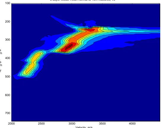
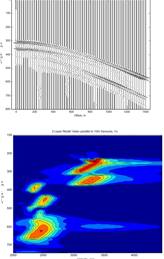
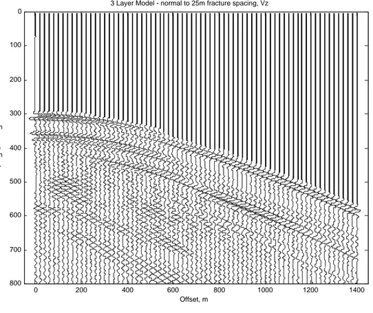
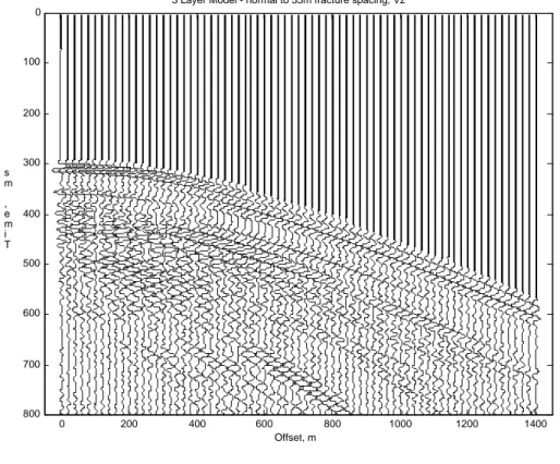
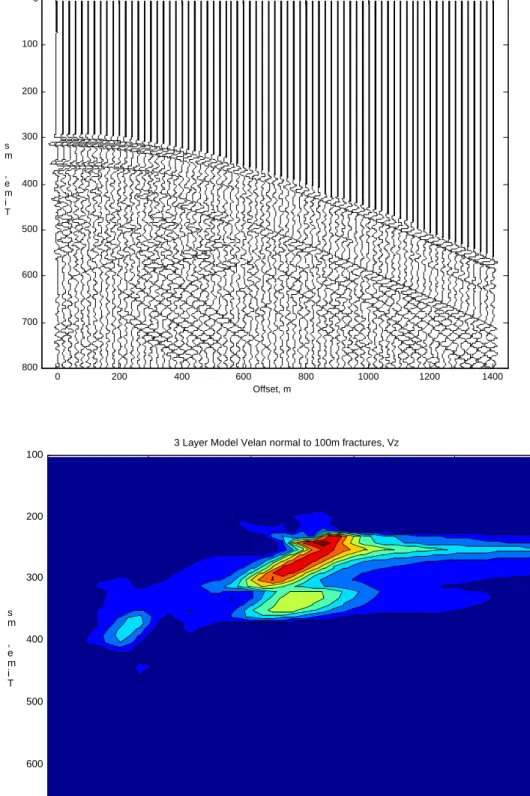
A three layer model was created to be able to isolate the various effects of P and S wave conversions in a fractured layer. The vertical component of velocity recorded over these simulations was used in this study. Two receiver lines were recorded – one normal to the fracture direction and one perpendicular to the fracture direction. Figure 1 shows the geometry and velocity distribution of the base elastic model. The second layer is then perturbed with six different fracture densities – no fractures, 10m, 25m, 35m, 50m and 100m spacing of fractures. The shot records showing the vertical component of velocity (Vz) are shown in the top (a) part of Figures 2-12 for different fracture densities and acquisition directions.
2.2
Five Layer Model
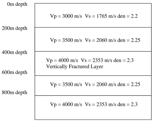
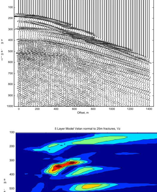
A five layer model was created to better isolate the reflections in time and to have reflections from other non-fractured layers. Both the pressure and Vz components were recorded for these simulations, but only the vertical component will be presented. As before, two receiver lines were recorded – one normal to the fracture direction and one perpendicular to the fracture direction. Figure 13 shows the geometry and velocity distribution of the base elastic model. The second layer is then perturbed with two fracture densities – no fractures, and a 25m spacing of fractures. The Vz shot record is shown in Figure 14a for the no fracture case. Figure 15a shows the Vz shot record for the case normal to the 25m fracture direction and Figure 16a is for the parallel case.
2.3
Modeling Observations
Each of the shot records were muted to remove the direct arrival from the source. It is quite apparent that after the reflection from the bottom of the fractured layer arrives, there are numerous scattered coda waves. There are only a few scattered waves immediately following the reflection from the top of the fractured layer. At first this may seem counterintuitive. However, it appears that most of the energy is bouncing around within the fractured layer rather than being immediately backscattered to the surface. Thus the reflection from the bottom of the fractured layer is still the shorter time path. It is also clear that coda waves on the traces recorded normal to the fractures are not very coherent. They seem to be scattered in many directions. On the other hand, the coda waves on the traces recorded parallel to the fractures look like reverberations of the fractured layer bottom event and share its moveout.
3
Velocity Spectra of Modeling Results
A conventional stacking velocity analysis (Taner and Kohler, 1969) was used to compute velocity spectra for the 3 and 5 layer model simulations since the focus of this study was not a detailed velocity
investigation. Higher order methods (e.g. Alkhalifah, 1997) could have been used in for a velocity anisotropy study. No attempt was made to study the velocities of the converted S waves, since that would have required common conversion point technology (Li, 2000; Audebert et al, 1999) and is beyond the scope this paper.
3.1
Velocity Spectra for the 3 Layer Model
The velocity spectra for each of the 3 layer model fracture cases were computed using 40 of the 71 offsets available. This corresponds to a far offset of 780m. The velocity spectra for each of the fracture spacing cases are shown in the bottom (b) part of Figures 2-12.
3.2
Velocity Spectra for the 5 Layer Model
As for the 3 layer model, the velocity spectra for each of the 5 layer model fracture cases were computed using 40 of the 71 offsets available. The velocity spectra for the no fracture case is shown in Figure 14b. Figure 15b shows the velocity spectra for the 25m normal to the fracture direction and Figure 16b shows the parallel case.
3.3
Observations on Model Velocity Spectra
It is quite apparent from the velocity spectra of the shot records acquired normal to the fracture direction, that virtually none of the ringing coda energy stacks coherently. In contrast, the spectra from the shot records parallel to the fractures exhibit quite a lot of coda energy which stacks in below the bottom of the reservoir event. This indicates that while there certainly may exist velocity functions that will stack the coda energy in the normal direction, they won’t be hyperbolic. From this result it is possible to conclude that conventional P wave processing will reduce the coda energy in the fracture normal direction. In the parallel direction, it is still possible that coda energy will make it through the stack process unscathed.
4
Stacking Analysis
Traces from the 5 layer model were used to test whether the coda wave energy will survive the stacking process. The stacking velocities used were picked from the computed velocity spectra in the previous section.
4.1
Stacking of the 5 Layer Model
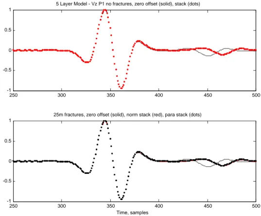
Figure 17a shows the zero offset (solid black) and stacked traces (dotted red) for the first reflector of the no fracture model. The traces are virtually identical. Figure 17b shows the same set of traces for the 25m fracture case. Again, these traces overlay perfectly. This should be no surprise since there are no changes between the models until the third layer.
Figure 18a shows the zero offset (solid black) and stacked traces (dotted red) for the second (top of fractured reservoir) reflector of the no fracture model. The traces are nearly identical. Figure 18b shows the same set of traces for the 25m fracture case in the normal direction. There are some small differences between the stack and the zero offset. Figure 18c shows the same set of traces for the 25m fracture case in the parallel direction. These traces are nearly identical.
Figure 19a shows the zero offset (solid black) and stacked traces (dotted red) for the third (bottom of fractured reservoir) reflector of the no fracture model. Again, the traces are nearly identical. Figure 19b shows the same set of traces for the 25m fracture case in the normal direction. Here there are some
significant differences especially later in the coda, after about sample number 840. Stacking has diminished the coda energy. Figure 19c shows the same set of traces for the 25m fracture case in the parallel direction. As before, these traces are nearly identical.
Figure 20a shows the zero offset (solid black) and stacked traces (dotted red) for the fourth (last) reflector of the no fracture model. As before, the stack and zero offset traces are nearly identical. Figure 20b shows the same set of traces for the 25m fracture case in the normal direction. In this case the stacked trace is larger in amplitude early on, but quickly gets out of phase with the zero offset trace. It then is attenuated with respect to the zero offset trace. Stacking has diminished the coda energy, especially late at late times. Figure 20c shows the same set of traces for the 25m fracture case in the parallel direction. This
time the traces are not identical. Early on the stacked trace is bigger than the zero offset trace and then is generally “close” to it. They stay nearly in phase with each other, unlike the normal direction case.
4.2
Observations on Stacking Analysis
The model stacking showed the following: 1) stacking had no effect on layers above the fractures, 2) stacking in the normal direction to the fractures diminished coda energy, 3) stacking in the direction parallel to the fractures affected much less or no damage to the coda energy. For each of these cases a single velocity function was used to stack the event. Since the velocity of the primary was used, in practice it is likely that the coda energy will be preserved in the parallel direction and diminished in the normal direction.
5
Transfer Function Estimation – Simple Input/Output Model
Signal processing theory has a rich literature describing how to obtain the impulse response or the transfer function of a system knowing only the input and outputs of a system. The transfer function of the system is “simply” deconvolved from the known responses. While many deconvolution formulations may be use, this paper uses Weiner deconvolution (see for example Yilmaz, 2000, or Robinson and Treitel, 1980).
5.1
Simple Convolutional Model for Transmission
The most simple example of a convolutional model is a single rock unit where a signal, i(t), is applied to its top surface and the seismic waves, o(t), are recorded on its bottom surface. The transfer function, h(t), transforms the input signal, i(t) to the output signal, o(t) by
)
(
)
(
)
(
t
h
t
o
t
i
∗
=
(1)where * represents convolution. Thus to get the transfer function, h(t), Weiner deconvolution is performed on o(t) using i(t). The function h(t) will completely describe the properties of the medium between the source and receiver. This model is appropriate for laboratory core measurements or perhaps cross well applications. However, surface seismic surveys are not pure transmission experiments, they are by design, reflection experiments.
5.2
Simple Convolutional Model for Reflection Events
The most simple reflection experiment is that of a 3 layer model, like Figure 1. A seismic source, s(t), transmits energy into the top layer. It propagates to the top of the first interface and is reflected upward as i(t). At the first interface it is also transmitted downward. The transmitted wave then reflects off the bottom of the next interface and is transmitted upward toward the surface where it is finally recorded as o(t). Using the same equation as Equation (1), h(t) does not represent the quite same phenomenon. This new transfer function contains the difference between the reflection and transmission coefficients at the top of the layer, a reflection coefficient at the bottom of the layer, and twice the path through the layer. If the resulting difference between these coefficients is a scalar, then disregarding the scalar, the transfer function is simply twice the propagation through the layer of interest.
As before, the transfer function, h(t), is obtained by Weiner deconvolution of the bottom of the layer reflection, o(t), and the top of the layer reflection, i(t). Disregarding the scalar amplitude, the function h(t) describes two propagation paths through the layer of interest.
5.3
Example Transfer Function – 5 Layer Model, Zero Offset, Single Wavelet
Zero offset traces are taken from the 5 layer model to demonstrate the case when it is possible to extract two complete reflections - one from an event above the layer of interest, and one from the bottom of the layer of interest. Figure 21a shows the extracted first reflection from the zero offset trace with no fractures in Figure 14a. Figure 21b shows the extracted reflection from the bottom of the third layer from the zero
offset trace with no fractures in Figure 14a. Figure 21c shows the computed transfer function. It is basically a single large pulse which has negative polarity showing that the reflection coefficient is negative. Its delay from zero time represents the travel time through the layer.
Figure 22a shows the extracted first reflection from the zero offset trace with 25m spacing fractures in Figure 14a. Figure 22b shows the extracted reflection from the bottom of the third layer from the zero offset trace with 25m fractures spacing in Figure 14a. Figure 22c shows the computed transfer function. It is a single negative pulse followed by a long ringy wave train. It represents the delay time of about 425 samples and the scattering property of the layer of interest.
5.4
Example Transfer Function – 5 Layer Model, Stacked, Single Wavelet
Stacked traces in the normal and parallel directions are taken from the 5 layer model to demonstrate again the case when it is possible to extract two complete reflections or wavelets. Figure 23a shows the extracted first reflection from the stacked trace with no fractures in Figure 14a. Figure 23b shows the extracted reflection from the bottom of the third layer from the stacked trace with no fractures in Figure 14a. Figure 21c shows the computed transfer function. It is virtually identical to the unstacked, zero offset case.
Figure 24a shows the extracted first reflection from the stacked trace in the normal direction with 25m spacing fractures in Figure 15a. Figure 24b shows the extracted reflection from the bottom of the third layer from the stacked trace in the normal direction with 25m fractures spacing in Figure 15a. Figure 24c shows the computed transfer function. It is a single large negative pulse followed by a short, lower amplitude ringy wave train. It represents the delay time of about 425 samples and the residual scattering after stacking of the layer of interest.
Figure 25a shows the extracted first reflection from the stacked trace in the parallel direction with 25m spacing fractures in Figure 16a. Figure 24b shows the extracted reflection from the bottom of the third layer from the stacked trace in the parallel direction with 25m fractures spacing in Figure 16a. Figure 24c shows the computed transfer function. It is a single negative pulse followed by a longer, higher amplitude ringy wave train. It represents the delay time of about 425 samples and the still present scattering after stacking of the layer of interest.
5.5
Observations on Single Event Transfer Functions
Providing that both entire reflection waveforms can be isolated, the transfer functions derived were effective at extracting both the time delay properties of the layer, and also the scattering coda effects from the layer as well.
6
Transfer Function Estimation – More Realistic Model
The examples shown in section 5 above were almost pathologic. In field data it is usually not clear where a reflection wavelet either begins or ends. So the methodology above must be amended to handle the more general case of a reflection series.
6.1
Seismic Reflection Convolutional Model
Ignoring noise, the surface seismic experiment can be represented as a seismic source, s(t), exciting the earth, e(t), and creating a reflection time series, x(t), which can be written as:
)
(
)
(
)
(
t
e
t
x
t
s
∗
=
(2)where e(t) is a sequence of reflectivity spikes corresponding to the travel times and acoustic impedances of each layer encounter along the path and * represents convolution. Making the appropriate assumptions (Yilmaz, 2000) about the randomness of the earth reflectivity series, e(t), the autocorrelation (
⊕
)
of the recorded seismogram, x(t), becomes:)
(
)
(
)
(
)
(
t
s
t
x
t
x
t
s
⊕
≈
⊕
(3)which is only related to the source wavelet at lags around zero. So we can estimate the autocorrelation of the source wavelet in a reflection series by taking the autocorrelation of the reflection series.
The source wavelet itself is not of interest, but rather the change of the wavelet above an interval and below it. So Equation (1) is still used, but i(t) is now the autocorrelation of a reflection series above the zone of interest. For o(t), the autocorrelation of the a reflection series below the zone of interest is used.
If the scattering properties of a particular interval is of interest, this process can be applied to a carefully chosen set of windows on the stacked seismic trace. Alternatively, this process can be used in a reconnaissance mode by sliding a moving set of windows down each trace and computing the transfer functions for each analysis window.
6.2
Autocorrelation of Single Events Example Using the 5 Layer Model
The autocorrelations of the stacked traces in the normal and parallel directions are taken from the 5 layer model as the first step to demonstrate using autocorrelations instead of the wavelets themselves. Figure 26a shows the autocorrelation of extracted first reflection from the stacked trace with no fractures in Figure 14a. Figure 26b shows the autocorrelation of the extracted reflection from the bottom of the third layer from the stacked trace with no fractures in Figure 14a. Figure 21c shows the positive lags of the computed transfer function. It is nearly a spike at zero lag. The travel time delay information was lost due to the use of the wavelet autocorrelations.
Figure 27a shows the autocorrelation of the extracted first reflection from the stacked trace in the normal direction with 25m spacing fractures in Figure 15a. Figure 27b shows the autocorrelation of the extracted reflection from the bottom of the third layer from the stacked trace in the normal direction with 25m fractures spacing in Figure 15a. Figure 27c shows the positive lags of the computed transfer function. It also is nearly a spike at zero lag and as before all of the travel time delay information is gone.
Figure 28a shows the autocorrelation of the extracted first reflection from the stacked trace in the parallel direction with 25m spacing fractures in Figure 16a. Figure 28b shows the autocorrelation of the extracted reflection from the bottom of the third layer from the stacked trace in the parallel direction with 25m fractures spacing in Figure 16a. Figure 28c shows the computed transfer function. It has a large zero lag value following by a ringing wave training capturing the scattered coda energy of the second wavelet.
6.3
Autocorrelation of Two Events Example Using the 5 Layer Model
Since the models generated did not contain realistically large numbers of reflections, it is not possible to fully test concept of estimating the source wavelets from windows containing many reflectors. However, as a first step, the autocorrelations of the zero offset traces containing two events in the normal and parallel directions were taken from the 5 layer model. Figure 29a shows the autocorrelation of extracted first and second reflections from the zero offset trace with no fractures in Figure 14a. Figure 29b shows the
autocorrelation of the extracted reflection from the bottom two P wave reflections from the zero offset trace with no fractures in Figure 14a. Both of these autocorrelation functions show prominent peaks at delay times corresponding to the time thickness of the layers. Figure 29c shows the positive lags of the computed transfer function. The transfer function is now a series of alternating spikes corresponding the time lags of the layer thicknesses.
Figure 30a shows the autocorrelation of the extracted first and second reflections from the zero offset trace with 25m spacing fractures in Figure 15a. Figure 30b shows the autocorrelation of the extracted reflection from the bottom two P wave reflections from the zero offset trace with 25m fracture spacing in Figure 15a. Figure 30c shows the positive lags of the computed transfer function. The transfer function is now much more ringy and only has hints of the alternating spikes of Figure 29c.
6.4
Windowed Autocorrelation of Two Events Example Using the 5 Layer Model
To extract the autocorrelation of the source wavelet in field data, only a subportion near the zero lag of the autocorrelation of the reflection time series can be used. For this example, the autocorrelations in section 6.3 are windowed to remove the peaks associated with the two layers. Figure 31a shows the windowed autocorrelation of extracted first and second reflections from the zero offset trace with no fractures. Figure 31b shows the windowed autocorrelation of the extracted reflection from the bottom two P wave reflections
from the zero offset trace with no fractures. Figure 31c shows the positive lags of the computed transfer function. The transfer function has now returned to a nearly a simple spike. Note that the time scale has changed on this plot from the previous figures.
Figure 32a shows the windowed autocorrelation of the extracted first and second reflections from the zero offset trace with 25m spacing fractures in Figure 15a. Figure 32b shows the windowed
autocorrelation of the extracted reflection from the bottom two P wave reflections from the zero offset trace with 25m fracture spacing in Figure 15a. Figure 32c shows the positive lags of the computed transfer function. The transfer function is again ringy.
6.5
Observations on Using a More Realistic Convolutional Model
Without the use of the autocorrelations in place of the extracted wavelets, this methodology would not be practical. It is extremely rare when reflectors are completely isolated in time. This section explored the use of the autocorrelation. Several observations can be made: 1) the general impulsive and ringy character of the transfer function using the extracted wavelets is preserved using the autocorrelation, 2) the specific characteristic of the transfer functions are different from their extracted wavelet counterparts as they should be, and 3) windowing of the autocorrelation functions before use in the deconvolution seems to reduce the effects of correlated reflectivity.
7
Application to Field Data
The PP preprocessed, prestack seismic traces from an ocean bottom cable survey were sorted into 9 CDP supergathers about 4 well locations. The survey is located in 80m water depth and was collected using an orthogonal acquisition geometry. The nominal fold is 144. The reservoir is located at about 2850m depth or at a two way time of about 2.3 seconds (sample 575). There are naturally occurring fractures in the reservoir that have high dip (60 to 80 degrees).
7.1
Azimuth Stacks
Azimuth stacks were created around four well locations in the survey. For each location, eighteen stacks of the data were made, one for every 10 degrees starting at 0 degrees (due East) all the way to 170 degrees (N80W). Both the nominal bearing and 180 degrees away azimuths were included. A range of +- 45 degrees about the nominal bearing of the stack was included. In addition, the offset range was limited to 2000m and less. The stacks for wells 3, 4, 5 and 7 are shown in Figures 34, 36, 38, and 40, respectively. The fold in each trace is roughly over 100 at bearings near zero and drops to over 30 at bearings near 90 degrees.
7.2
Transfer Function Computation
The transfer function estimation methodology described in section 6.1 was used to create a matrix of functions characterizing the azimuthal and temporal variation of the traces in the azimuth stacks. Figure 33 shows the sliding analysis configuration used. The autocorrelation of a 100 sample window of the top of the seismic trace was used as the input. The autocorrelation of another 100 sample window, located 50 samples below the first window, was used as the output function. The transfer function was determined for this analysis time and then associated with a bin in the transfer function matrix. The absolute value of each sample of the transfer function was taken (called rectifying) and the positive lags of the function were placed in the bin of the matrix corresponding to the time of this analysis window and the azimuth of the stacked seismic trace. The analysis window was then moved 20 samples later in time and the process was repeated until each time window and azimuth trace were analyzed.
The transfer function matrices for wells 3, 4, 5, and 7 are shown in Figures 35, 37, 39 and 41. A quick review of these matrices reveals quite a lot of variability of the transfer functions both temporally and azimuthally.
7.3
Moment of Transfer Function Computation
Because it is difficult to assimilate the entire grid of rectified transfer functions, each function was reduced to a single number, the moment of the transfer function. The moment value, m, used is given by
)
(
0 2l
h
l
m
n l∑
=≡
(4)where n is half the number of points in the transfer function. For a transfer function consisting of a single spike the moment value is zero. For a long ringy transfer function the moment value is large. So the moment value is a direct indication of a ringing transfer function.
The matrix of moment values for each of the four wells is shown in Figure 42. For visual clarity, the increment between analysis windows was decreased from every 20 samples to every 5 samples.
7.4
Observations on Analysis of Field Data
No investigation of optimal parameterization has performed yet so it is difficult to know whether the parameters chosen provide an optimal view of the fractured coda energy. The rectified transfer functions and transfer function moments indicate several trends: 1) at shallow times (samples 250 to 300) there appears to be high moments which may be associated with low fold azimuths near 90 degrees, 2) well 3 shows a fairly consistent fracture orientation at 140 degrees at nearly all times, 3) wells 5 and 7 show high moments in the reservoir interval (samples 500 to 650) at nearly all azimuths, 4) wells 5 and 7 show fairly consistent low moments in the interval 400 to 500 samples, and 5) well 4 shows high moments at 140 degrees in the reservoir interval (samples 500 to 600).
8
Conclusions
A methodology was developed to compute the interval transfer function for seismic reflection traces which captures the amount of scattering in the interval. The method was tested on both model and field data with encouraging results. The model data indicate that ringing coda waves are generated over parallel vertically fractured layers. These coda waves tend to stack out if acquired normal to the fracture orientation. Data acquired parallel to the fracture orientation tend not to be attenuated by stacking. Transfer functions acquired from stacked data oriented normal to the fractures tend to more impulsive. Those from the parallel direction tend to be quite ringy. The results of processing field data show transfer functions possibly indicative of fractured zones. Some time ranges show strong azimuthal variations while others show less azimuthal variation. Additional work needs to be done to quantitatively calibrate these measurements to fracture density.
9
Acknowledgments
The authors wish to thank Joongmoo Byun for performing all of the 3D elastic finite difference modeling. This work was supported by the Earth Resources Laboratory Founding Members, the Department of Energy Grant number DE-FC26-02NT15346, and by ENI S.p.A. AGIP.
References
T. Alkhalifah. Velocity analysis using nonhyperbolic moveout in transversely anisotropic media. Geophysics 62:1839-1854.
F. Audebert, P.Y. Granger, and A. Herrenschmidt. CCP-Scan technique: True common conversion point sorting and converted-wave velocity analysis solved by PP and PS pre-stack depth migration. In Expanded Abstracts, Tulsa, 1999, Soc. Of Expl. Geophys.
T.M. Daley, K.T. Nihei, L.R. Myer, J.H. Queen, M. Fortuna, and J. Murphy. Numerical modeling of scattering from discrete fracture zones in a San Juan Basin gas reservoir. In Expanded Abstracts, Tulsa, 2002, Soc. Of Expl. Geophys.
J. Gaiser, E. Loinger, H. Lynn and L. Vetri. Birefringence analysis at Emilio field for fracture characterization. First Break, 20:505-514, Aug. 2002.
Xiang-Yang Li. Converted-wave velocity analysis: searching for Vc and _. Presented at EAGE meeting, Glasgow, Scotland, Jun. 2000.
Subhashis Mallick, Kenneth L. Craft, Laurent J. Meister, and Ronald E. Chambers. Determination of the principal directions of azimuthal anisotropy from P-wave seismic data. Geophysics 63(2):692-706, Mar.-Apr. 1998.
Seiji Nakagawa, Kurt T. Nihei and Larry R. Myer. Numerical simulation of 3D elastic wave scattering off a layer containing parallel periodic fractures. In Expanded Abstracts, Tulsa, 2002, Soc. Of Expl. Geophys.
Enders Robinson and Sven Treitel. Geophysical Signal Analysis. 1980, Prentice Hall.
C. Schultz. Enhanced backscattering of seismic waves from irregular interfaces. PhD thesis, MIT, Cambridge, MA, 1994.
M. T. Taner and F. Koehler. Velocity spectra – digital computer derivation and applications of velocity functions. Geophysics 39:859-881, 1969.
Özdo_an Yilmaz. Processing, inversion, and interpretation of seismic data. Society of Exploration Geophysicists. 2000.
Figure 1. Three layer model showing one configuration of fractures.
Vp = 3000 m/s Vs= 1765 m/s Dens = 2.2 g/cc
Vp = 4000 m/s Vs = 2353 m/s Dens = 2.3 g/cc
Vertically Fractured Layer Vp = 3000 m/s Vs= 1765 m/s Dens = 2.2 g/cc
0m depth
1000m depth
1100m depth
1350m depth
2000 2500 3000 3500 4000 100 200 300 400 500 600 700
3 Layer Model Velan no fractures, Vz
Velocity, m/s T i m e , m s 0 100 200 300 400 500 600 700 800 0 200 400 600 800 1000 1200 1400 3 Layer Model - normal to 10m fracture spacing, Vz
T i m e , m s Offset, m 0 100 200 300 m s
Figure 2. Three layer model with no fractures – a) seismograms (
velocity analysis (bottom).
2000 2500 3000 3500 4000 100 200 300 400 500 600 700
3 Layer Model Velan normal to 10m fractures, Vz
Velocity, m/s T i m e , m s
Figure 3. Three layer model with acquisition normal to the 10m spacing fractures
– a) seismograms (top), b) velocity analysis (bottom).
0 100 200 300 400 500 600 700 800 0 200 400 600 800 1000 1200 1400 3 Layer Model - parallel to 10m fracture spacing, Vz
T i m e , m s Offset, m 2000 2500 3000 3500 4000 100 200 300 400 500 600 700
3 Layer Model Velan parallel to 10m fractures, Vz
Velocity, m/s T i m e , m s
Figure 4. Three layer model with acquisition parallel to the 10m spacing
fractures – a) seismograms (top), b) velocity analysis (bottom).
0 100 200 300 400 500 600 700 800 0 200 400 600 800 1000 1200 1400
3 Layer Model - normal to 25m fracture spacing, Vz
T i m e , m s Offset, m 2000 2500 3000 3500 4000 100 200 300 400 500 600 700
3 Layer Model Velan normal to 25m fractures, Vz
Velocity, m/s T i m e , m s
0 100 200 300 400 500 600 700 800 0 200 400 600 800 1000 1200 1400 3 Layer Model - parallel to 25m fracture spacing, Vz
T i m e , m s Offset, m 2000 2500 3000 3500 4000 100 200 300 400 500 600 700
3 Layer Model Velan parallel to 25m fractures, Vz
Velocity, m/s T i m e , m s
Figure 6. Three layer model with acquisition parallel to the 25m spacing
fractures – a) seismograms (top), b) velocity analysis (bottom).
0 100 200 300 400 500 600 700 800 0 200 400 600 800 1000 1200 1400 3 Layer Model - normal to 35m fracture spacing, Vz
T i m e , m s Offset, m 2000 2500 3000 3500 4000 100 200 300 400 500 600 700
3 Layer Model Velan normal to 35m fractures, Vz
Velocity, m/s T i m e , m s
0 100 200 300 400 500 600 700 800 0 200 400 600 800 1000 1200 1400 3 Layer Model - parallel to 35m fracture spacing, Vz
T i m e , m s Offset, m 2000 2500 3000 3500 4000 100 200 300 400 500 600 700
3 Layer Model Velan parallel to 35m fractures, Vz
Velocity, m/s T i m e , m s
Figure 8. Three layer model with acquisition parallel to the 35m spacing
fractures – a) seismograms (top), b) velocity analysis (bottom).
0 100 200 300 400 500 600 700 800 0 200 400 600 800 1000 1200 1400 3 Layer Model - normal to 50m fracture spacing, Vz
T i m e , m s Offset, m 2000 2500 3000 3500 4000 100 200 300 400 500 600 700
3 Layer Model Velan normal to 50m fractures, Vz
Velocity, m/s T i m e , m s
Figure 9. Three layer model with acquisition normal to the 50m spacing fractures
– a) seismograms (top), b) velocity analysis (bottom).
0 100 200 300 400 500 600 700 800 0 200 400 600 800 1000 1200 1400 3 Layer Model - parallel to 50m fracture spacing, Vz
T i m e , m s Offset, m 2000 2500 3000 3500 4000 100 200 300 400 500 600 700
3 Layer Model Velan parallel to 50m fractures, Vz
Velocity, m/s T i m e , m s
Figure 10. Three layer model with acquisition parallel to the 50m spacing
fractures – a) seismograms (top), b) velocity analysis (bottom).
0 100 200 300 400 500 600 700 800 0 200 400 600 800 1000 1200 1400 3 Layer Model - normal to 100m fracture spacing, Vz
T i m e , m s Offset, m 2000 2500 3000 3500 4000 100 200 300 400 500 600 700
3 Layer Model Velan normal to 100m fractures, Vz
Velocity, m/s T i m e , m s
Figure 11. Three layer model with acquisition normal to the 100m spacing
fractures – a) seismograms (top), b) velocity analysis (bottom).
0 100 200 300 400 500 600 700 800 0 200 400 600 800 1000 1200 1400 3 Layer Model - parallel to 100m fracture spacing, Vz
T i m e , m s Offset, m 2000 2500 3000 3500 4000 100 200 300 400 500 600 700
3 Layer Model Velan parallel to 100m fractures, Vz
Velocity, m/s T i m e , m s
Figure 12. Three layer model with acquisition parallel to the 100m spacing
fractures – a) seismograms (top), b) velocity analysis (bottom).
Figure 13. Five Layer model geometry. Receiver spacing is 20m, sample interval is
0.5ms.
Vp = 3000 m/s Vs = 1765 m/s den = 2.2
Vp = 3500 m/s Vs = 2060 m/s den = 2.25
Vp = 4000 m/s Vs = 2353 m/s den = 2.3
Vertically Fractured Layer
Vp = 3500 m/s Vs = 2060 m/s den = 2.25
Vp = 4000 m/s Vs = 2353 m/s den = 2.3
0m depth
200m depth
400m depth
600m depth
800m depth
0 100 200 300 400 500 600 700 800 900 1000 0 200 400 600 800 1000 1200 1400 5 Layer Model - no fractures, Vz
T i m e , m s Offset, m 2000 2500 3000 3500 4000 100 200 300 400 500 600 700 800 900
5 Layer Model Velan no fractures, Vz
Velocity, m/s T i m e , m s
Figure 14. Five layer model with no fractures – a) seismograms (top), b)
velocity analysis (bottom).
0 100 200 300 400 500 600 700 800 900 1000 0 200 400 600 800 1000 1200 1400 5 Layer Model - normal to 25m fracture spacing, Vz
T i m e , m s Offset, m 2000 2500 3000 3500 4000 100 200 300 400 500 600 700 800 900
5 Layer Model Velan normal to 25m fractures, Vz
Velocity, m/s T i m e , m s
0 100 200 300 400 500 600 700 800 900 1000 0 200 400 600 800 1000 1200 1400 5 Layer Model - parallel to 25m fracture spacing, Vz
T i m e , m s Offset, m 2000 2500 3000 3500 4000 100 200 300 400 500 600 700 800 900
5 Layer Model Velan parallel to 25m fractures, Vz
Velocity, m/s T i m e , m s
Figure 16. Five layer model with acquisition parallel to the 25m spacing
fractures – a) seismograms (top), b) velocity analysis (bottom).
250 300 350 400 450 500 -1 -0.5 0 0.5 1
5 Layer Model - Vz P1 no fractures, zero offset (solid), stack (dots)
250 300 350 400 450 500 -1 -0.5 0 0.5 1
25m fractures, zero offset (solid), norm stack (red), para stack (dots)
Time, samples
Figure 17. Five layer model first reflection. a) No
fracture case (top) - zero offset trace (black), stacked
trace (red). b) Fracture spacing 25m (bottom) – zero
offset trace (black), stacked trace (red).
500 550 600 650 700 750 -1 -0.5 0 0.5 1
5 Layer Model - Vz P2 no fractures, zero offset (solid), stack (dots)
500 550 600 650 700 750 -1 -0.5 0 0.5 1
25m fractures, zero offset (solid), norm stack (dots)
500 550 600 650 700 750 -1 -0.5 0 0.5 1
25m fractures, zero offset (solid), para stack (dots)
Time, samples
Figure 18. Five layer model second reflection. a) No fracture case (top) - zero offset
trace (black), stacked trace (red). b) Acquisition normal to fracture spacing of 25m
(middle) – zero offset trace (black), stacked trace (red). c) Acquisition parallel to
fracture spacing of 25m (bottom)– zero offset trace (black), stacked trace (red).
700 750 800 850 900 950 -2
-1 0 1
5 Layer Model - Vz P3 no fractures, zero offset (solid), stack (dots)
700 750 800 850 900 950 -1 -0.5 0 0.5 1
25m fractures, zero offset (solid), norm stack (dots)
700 750 800 850 900 950 -1 -0.5 0 0.5 1
25m fractures, zero offset (solid), para stack (red)
Time, samples
Figure 19. Five layer model third reflection. a) No fracture case (top) - zero offset
trace (black), stacked trace (red). b) Acquisition normal to fracture spacing of 25m
(middle) – zero offset trace (black), stacked trace (red). c) Acquisition parallel to
fracture spacing of 25m (bottom) – zero offset trace (black), stacked trace (red).
950 1000 1050 1100 1150 -1 -0.5 0 0.5 1
5 Layer Model - Vz P4 no fractures, zero offset (solid), stack (dots)
950 1000 1050 1100 1150
-2 -1 0 1
25m fractures, zero offset (solid), norm stack (dots)
950 1000 1050 1100 1150
-2 -1 0 1
25m fractures, zero offset (solid), para stack (dots)
Time, samples
Figure 20. Five layer model fourth reflection. a) No fracture case (top) - zero offset
trace (black), stacked trace (red). b) Acquisition normal to fracture spacing of 25m
(middle) – zero offset trace (black), stacked trace (red). c) Acquisition parallel to
fracture spacing of 25m (bottom) – zero offset trace (black), stacked trace (red).
0 100 200 300 400 500 600 700 800 900 1000 -4 -2 0 2 4x 10
10 5 Layer Model - no fractures - Vz
0 100 200 300 400 500 600 700 800 900 1000 -1 -0.5 0 0.5 1x 10 10 0 100 200 300 400 500 600 700 800 900 1000 -0.03 -0.02 -0.01 0 0.01 Transfer Function - P1 to P3 Time, samples
Figure 21. Zero offset traces from the five layer model with no fractures. a) first
reflection as input wavelet (top), b) third reflection as output wavelet (middle), c) transfer
function taking the input to the output wavelet (bottom)
0 100 200 300 400 500 600 700 800 900 1000 -4 -2 0 2 4x 10 10
5 Layer Model - 25m fractures - Vz
0 100 200 300 400 500 600 700 800 900 1000 -1 -0.5 0 0.5 1x 10 10 0 100 200 300 400 500 600 700 800 900 1000 -0.04 -0.02 0 0.02 Transfer Function - P1 to P3 Time, samples
Figure 22. Zero offset traces from the five layer model with 25m fracture spacing. a) first
reflection as input wavelet (top), b) third reflection as output wavelet (middle), c) transfer
function taking the input to the output wavelet (bottom)
0 200 400 600 800 1000 1200 -1 -0.5 0 0.5 1
5 Layer Model stacked - no fractures - Vz
0 200 400 600 800 1000 1200 -2 -1 0 1 0 200 400 600 800 1000 1200 -0.15 -0.1 -0.05 0 0.05 Transfer Function - P1 to P3 Time, samples
Figure 23. Stacked offset traces from the five layer model with no fractures. a) first
reflection as input wavelet (top), b) third reflection as output wavelet (middle), c) transfer
function taking the input to the output wavelet (bottom)
0 200 400 600 800 1000 1200 -1 -0.5 0 0.5 1
5 Layer Model stacked - normal to 25m fractures - Vz
0 200 400 600 800 1000 1200 -1 -0.5 0 0.5 1 0 200 400 600 800 1000 1200 -0.1 -0.05 0 0.05 0.1 Transfer Function - P1 to P3 Time, samples
Figure 24. Stacked offset traces from the five layer model with acquisition normal to the
25m fracture spacing. a) first reflection as input wavelet (top), b) third reflection as
output wavelet (middle), c) transfer function taking the input to the output wavelet
(bottom)
0 200 400 600 800 1000 1200 -1 -0.5 0 0.5 1
5 Layer Model stacked - parallel to 25m fractures - Vz
0 200 400 600 800 1000 1200 -1 -0.5 0 0.5 1 0 200 400 600 800 1000 1200 -0.2 -0.1 0 0.1 0.2 Transfer Function - P1 to P3 Time, samples
Figure 25. Stacked offset traces from the five layer model with acquisition parallel to the
25m fracture spacing. a) first reflection as input wavelet (top), b) third reflection as
output wavelet (middle), c) transfer function taking the input to the output wavelet
(bottom)
0 100 200 300 400 500 600 700 800 900 1000 -20 -10 0 10 20
5 Layer Model stacked, autoc. - no fractures - Vz
0 100 200 300 400 500 600 700 800 900 1000 -20 -10 0 10 20 0 100 200 300 400 500 600 700 800 900 1000 -0.05 0 0.05 0.1 0.15 Transfer Function - P1 to P3 Time, samples
Figure 26. Autocorrelation of the stacked traces from the five layer model with no
fractures. a) first reflection as input wavelet (top), b) third reflection as output wavelet
(middle), c) transfer function taking the input to the output wavelet (bottom)
0 100 200 300 400 500 600 700 800 900 1000 -20 -10 0 10 20
5 Layer Model stacked, autoc. - normal to 25m fractures - Vz
0 100 200 300 400 500 600 700 800 900 1000 -20 0 20 40 0 100 200 300 400 500 600 700 800 900 1000 -0.05 0 0.05 0.1 0.15 Transfer Function - P1 to P3 Time, samples
Figure 27. Autocorrelation of the stacked traces from the five layer model with
acquisition normal to the 25m fracture spacing. a) first reflection as input wavelet (top),
b) third reflection as output wavelet (middle), c) transfer function taking the input to the
output wavelet (bottom)
0 100 200 300 400 500 600 700 800 900 1000 -20 -10 0 10 20
5 Layer Model stacked, autoc. - parallel to 25m fractures - Vz
0 100 200 300 400 500 600 700 800 900 1000 -20 -10 0 10 20 0 100 200 300 400 500 600 700 800 900 1000 -0.1 0 0.1 0.2 0.3 Transfer Function - P1 to P3 Time, samples
Figure 28. Autocorrelation of the stacked traces from the five layer model with
acquisition parallel to the 25m fracture spacing. a) first reflection as input wavelet (top),
b) third reflection as output wavelet (middle), c) transfer function taking the input to the
output wavelet (bottom)
0 500 1000 1500 2000 2500 -2 0 2 4x 10 22
5 Layer Model - 2 refl., full autoc. - no fractures, Vz.
0 500 1000 1500 2000 2500 -2 -1 0 1 2x 10 21 0 200 400 600 800 1000 1200 -0.01 -0.005 0 0.005 0.01 Transfer Function - P1 to P3 Time, samples
Figure 29. Autocorrelation of the zero offset traces from the five layer model with no
fractures. a) first and second reflections as input wavelet (top), b) third and fourth
reflections as output wavelet (middle), c) transfer function taking the input to the output
wavelet (bottom)
0 500 1000 1500 2000 2500 -2 0 2 4x 10 22
5 Layer Model - 2 refl., full autoc. - parallel 25m fractures, Vz.
0 500 1000 1500 2000 2500 -2 0 2 4x 10 21 0 200 400 600 800 1000 1200 -0.02 -0.01 0 0.01 0.02 Transfer Function - P1 to P3 Time, samples
Figure 30. Autocorrelation of the zero offset traces from the five layer model with 25m
fracture spacing. a) first and second reflections as input wavelet (top), b) third and fourth
reflections as output wavelet (middle), c) transfer function taking the input to the output
wavelet (bottom)
0 100 200 300 400 500 600 -2 0 2 4x 10 22
5 Layer Model - 2 refl., autoc. - no fractures, Vz.
0 100 200 300 400 500 600 -2 -1 0 1 2x 10 21 0 50 100 150 200 250 300 -5 0 5 10 x 10-3 Transfer Function - P1 to P3 Time, samples
Figure 31. Windowed autocorrelation of the zero offset traces from the five layer model
with no fractures. a) first and second reflections as input wavelet (top), b) third and fourth
reflections as output wavelet (middle), c) transfer function taking the input to the output
wavelet (bottom)
0 100 200 300 400 500 600 -2 0 2 4x 10 22
5 Layer Model - 2 refl., autoc. - parallel 25m fractures, Vz.
0 100 200 300 400 500 600 -2 0 2 4x 10 21 0 50 100 150 200 250 300 -0.02 -0.01 0 0.01 0.02 Transfer Function - P1 to P3 Time, samples
Figure 32. Windowed autocorrelation of the zero offset traces from the five layer model
with 25m fracture spacing. a) first and second reflections as input wavelet (top), b) third
and fourth reflections as output wavelet (middle), c) transfer function taking the input to
the output wavelet (bottom)
100 200 300 400 500 600 700 800 T i m e , s a m p l e s
Figure 33. Schematic diagram showing the analysis windows to compute the transfer
functions of the field data. The input and out areas were chosen as 100 samples long for
this figure and the analysis window was chosen as 50 samples. The transfer function is
estimates for the gap (or area) between the input and output areas. The analysis is then
moved down the trace to create a transfer function for windows covering the entire trace.
100 samples of trace used as input area
100 samples of trace used as output area
50 samples representing analysis window
0 100 200 300 400 500 600 700 800 900 0 20 40 60 80 100 120 140 160 180
Well 3 - Azimuthal Stacks of 9 CDPs
T i m e , s a m p l e s Bearing, deg
Figure 34. Azimuthal stacks of traces in a 3 bin by 3 bin CDP gather around well 3. Each
trace is the stacked results of all traces with a shot to receiver azimuth direction within
+/-45° of the labeled bearing and +/- +/-45° of the opposite (180° from the bearing) direction.
0 20 40 60 80 100 120 140 160 180 250 300 350 400 450 500 550 600 650 700 Bearing, deg S t a r t T i m e o f A n a l y s i s W i n d o w , s a m p
Summary of Transfer Functions for Well 3
Figure 35. Summary of the computed transfer functions for well 3. The absolute values
of the transfer function for only the positive lags are plotted in each cell of the matrix.
The vertical blue lines separate each cell horizontally into the azimuthal stack directions
(bearing) corresponding to Figure 34. Each trace in Figure 34 is analyzed using an input
and output time series 100 samples long each, with separated by a 50 sample long
analysis window. Thus, the result in the bin {x = 10 degrees bearing, y = starting time
250 sample} is the transfer function for the input time series from sample 150 to 250,
output time series from sample 300 to 400, taken from the first trace of Figure 34.
0 100 200 300 400 500 600 700 800 900 0 20 40 60 80 100 120 140 160 180
Well 4 - Azimuthal Stacks of 9 CDPs
T i m e , s a m p l e s Bearing, deg
Figure 36. Azimuthal stacks of traces in a 3 bin by 3 bin CDP gather around well 4. Each
trace is the stacked results of all traces with a shot to receiver azimuth direction within
+/-45° of the labeled bearing and +/- +/-45° of the opposite (180° from the bearing) direction.
0 20 40 60 80 100 120 140 160 180 250 300 350 400 450 500 550 600 650 700 Bearing, deg S t a r t T i m e o f A n a l y s i s W i n d o w , s a m p
Summary of Transfer Functions for Well 4
Figure 37. Summary of the computed transfer functions for well 4. The absolute values
of the transfer function for only the positive lags are plotted in each cell of the matrix.
The vertical blue lines separate each cell horizontally into the azimuthal stack directions
(bearing) corresponding to Figure 36. Each trace in Figure 36 is analyzed using an input
and output time series 100 samples long each, with separated by a 50 sample long
analysis window. Thus, the result in the bin {x = 10 degrees bearing, y = starting time
250 sample} is the transfer function for the input time series from sample 150 to 250,
output time series from sample 300 to 400, taken from the first trace of Figure 36.
0 100 200 300 400 500 600 700 800 900 0 20 40 60 80 100 120 140 160 180
Well 5 - Azimuthal Stacks of 9 CDPs
T i m e , s a m p l e s Bearing, deg
Figure 38. Azimuthal stacks of traces in a 3 bin by 3 bin CDP gather around well 5. Each
trace is the stacked results of all traces with a shot to receiver azimuth direction within
+/-45° of the labeled bearing and +/- +/-45° of the opposite (180° from the bearing) direction.
0 20 40 60 80 100 120 140 160 180 250 300 350 400 450 500 550 600 650 700 Bearing, deg S t a r t T i m e o f A n a l y s i s W i n d o w , s a m p
Summary of Transfer Functions for Well 5
Figure 39. Summary of the computed transfer functions for well 5. The absolute values
of the transfer function for only the positive lags are plotted in each cell of the matrix.
The vertical blue lines separate each cell horizontally into the azimuthal stack directions
(bearing) corresponding to Figure 38. Each trace in Figure 38 is analyzed using an input
and output time series 100 samples long each, with separated by a 50 sample long
analysis window. Thus, the result in the bin {x = 10 degrees bearing, y = starting time
250 sample} is the transfer function for the input time series from sample 150 to 250,
output time series from sample 300 to 400, taken from the first trace of Figure 38.
0 100 200 300 400 500 600 700 800 900 0 20 40 60 80 100 120 140 160 180
Well 7 - Azimuthal Stacks of 9 CDPs
T i m e , s a m p l e s Bearing, deg
Figure 40. Azimuthal stacks of traces in a 3 bin by 3 bin CDP gather around well 7. Each
trace is the stacked results of all traces with a shot to receiver azimuth direction within
+/-45° of the labeled bearing and +/- +/-45° of the opposite (180° from the bearing) direction.
0 20 40 60 80 100 120 140 160 180 250 300 350 400 450 500 550 600 650 700 Bearing, deg S t a r t T i m e o f A n a l y s i s W i n d o w , s a m p
Summary of Transfer Functions for Well 7