HAL Id: hal-01476103
https://hal.laas.fr/hal-01476103
Submitted on 24 Feb 2017
HAL is a multi-disciplinary open access archive for the deposit and dissemination of sci-entific research documents, whether they are pub-lished or not. The documents may come from teaching and research institutions in France or abroad, or from public or private research centers.
L’archive ouverte pluridisciplinaire HAL, est destinée au dépôt et à la diffusion de documents scientifiques de niveau recherche, publiés ou non, émanant des établissements d’enseignement et de recherche français ou étrangers, des laboratoires publics ou privés.
network characterizations ONTIC: D4.3
Juliette Dromard, Véronique Baudin, Philippe Owezarski, Alberto Mozo
Velasco, Bruno Ordozgoiti, Sandra Gomez Canaval
To cite this version:
Juliette Dromard, Véronique Baudin, Philippe Owezarski, Alberto Mozo Velasco, Bruno Ordozgoiti, et al.. Experimental evaluation of algorithms for online network characterizations ONTIC: D4.3. LAAS/CNRS; UPM. 2017. �hal-01476103�
Online Network Traffic
Characterization
Deliverable
Experimental evaluation of algorithms for online network
characterizations
ONTIC Project
(GA number 619633)
Deliverable D4.3
Dissemination Level: PUBLIC
Authors
Dromard, Juliette; Baudin, Véronique; Owezarski, Philippe
LAAS-CNRS
Mozo Velasco, Alberto; Ordozgoiti, Bruno; Gómez Canaval Sandra
UPM
Version
ONTIC_D4.3.2017.02.10.1.1.final
!
!
Version History
Previous
version
Modification
date
Modified by
Summary
0.1
2016.12.22
CNRS
1
stdraft version
0.2
2017.01.18
SATEC
Integration of SATEC
Review
0.3
2017.01.25
POLITO
Integration of
POLITO Review
0.4
2017.02.09
POLITO
SATEC
Review
1.0 final
2017.02.10
UPM
Integration of UPM
inputs
1.1 final
2017.02.14
UPM
3 minor typos
corrected
Quality Assurance:
Name
Quality Assurance
Manager
Alberto Mozo (UPM)
Reviewer #1
Miguel Ángel López (SATEC)
Reviewer #2
Daniele Apiletti (POLITO)
Copyright © 2017, ONTIC Consortium
The ONTIC Consortium (http://www.http://ict-ontic.eu/) grants third parties the right to use and distribute all or parts of this document, provided that the ONTIC project and the document
are properly referenced.
THIS DOCUMENT IS PROVIDED BY THE COPYRIGHT HOLDERS AND CONTRIBUTORS "AS IS" AND ANY EXPRESS OR IMPLIED WARRANTIES, INCLUDING, BUT NOT LIMITED TO, THE IMPLIED
WARRANTIES OF MERCHANTABILITY AND FITNESS FOR A PARTICULAR PURPOSE ARE DISCLAIMED. IN NO EVENT SHALL THE COPYRIGHT OWNER OR CONTRIBUTORS BE LIABLE FOR
ANY DIRECT, INDIRECT, INCIDENTAL, SPECIAL, EXEMPLARY, OR CONSEQUENTIAL DAMAGES (INCLUDING, BUT NOT LIMITED TO, PROCUREMENT OF SUBSTITUTE GOODS OR SERVICES; LOSS OF USE, DATA, OR PROFITS; OR BUSINESS INTERRUPTION) HOWEVER CAUSED AND ON
ANY THEORY OF LIABILITY, WHETHER IN CONTRACT, STRICT LIABILITY, OR TORT (INCLUDING NEGLIGENCE OR OTHERWISE) ARISING IN ANY WAY OUT OF THE USE OF THIS
Table of Contents
1
E
XECUTIVES
UMMARY10
2
A
CRONYMS11
3
I
NTENDEDA
UDIENCE13
4
G
ROUNDT
RUTHG
ENERATION14
4.1 List and description of generated anomalies... 15
4.1.1 Network recognition anomalies ... 15
4.1.2 Attacks... 18
4.2 Implementation ... 21
4.3 Selection of the ONTS dataset ... 22
4.3.1 Visualizing existing traces ... 22
4.4 Used Tools ... 24
4.4.1 Common Research Emulator (CORE) ... 24
4.4.2 Domain Information Groper (Dig) ... 24
4.4.3 Network Mapper (Nmap) ... 24
4.4.4 Hping3 ... 24 4.4.5 Nping ... 24 4.4.6 Hydra ... 25 4.4.7 Ncrack ... 25 4.4.8 Wireshark/Tcpdump ... 25 4.5 Traces generation ... 25 4.5.1 Discovery anomalies ... 25 4.5.2 Attacks... 26
4.6 Ground truth use and dissemination ... 28
5
N
ETWORKA
NOMALY ANDI
NTRUSIOND
ETECTIONA
LGORITHMS29
5.1 Definition of an anomaly ... 305.2 Data preprocessing ... 32
6
T
HE DISCRETE TIME SLIDING WINDOW33
6.1.1 Description of the aggregation levels and their associated features ... 346.1.2 Feature space normalization ... 35
6.2 The clustering step ... 36
6.3 Anomaly identification ... 38
6.4 Distributed implementation of our solution using Spark Streaming ... 39
6.4.1 Spark Streaming ... 39
5/93
6.5 Validation of our solution using the ground truth ... 40
7
E
XPERIMENTATION AND VALIDATION ON THEG
OOGLEC
LOUD PLATFORM43
7.1 Cluster configuration ... 437.2 Key performance considerations ... 43
7.2.1 Tuning resource allocation ... 43
7.2.2 Level of parallelism ... 45
7.2.3 Serialization ... 45
7.3 Multi-Aggreg-ORUNADA stages ... 45
7.4 Performance tests of our solution implementation using the Google DataProc ... 47
7.4.1 Impact of the level of parallelism ... 47
7.4.2 Impact of the size of the cluster ... 48
7.4.3 Discussion ... 49
8
N
ETWORK TRAFFIC FORECASTING50
8.1 Problem setting ... 508.2 Modeling exponentially wide context efficiently ... 50
8.3 Coarse-grained long-term forecasts ... 51
8.4 Convolutional neural networks ... 52
8.5 Experimental results ... 52
8.5.1 ANNs and CNNs at different time scales ... 54
8.5.2 The effect of context... 57
8.6 Conclusions ... 58
9
P
ROACTIVE NETWORK CONGESTION CONTROL AND AVOIDANCE59
9.1 Scope ... 599.2 Problem setting ... 61
9.3 Problem solution ... 65
9.4 Forecasting Max-min fair rate assignments ... 66
9.4.1 Training and testing datasets ... 67
9.4.2 Linear regression ... 69
9.4.3 Artificial neural networks ... 69
9.5 Experiments ... 70
9.6 Conclusions ... 75
10
D
ETECTION OF ANOMALIES IN CLOUD INFRASTRUCTURE USINGD
EEPN
EURALN
ETWORKS76
10.1 Problem setting ... 7710.2 Convolutional neural networks for noisy neighbour detection ... 78
10.3 Experiments ... 79
10.4 Conclusions ... 80
11
R
EFERENCES81
6/93
A
NNEXB
G
ROUNDT
RUTHG
ENERATION86
Annex C Scan OS host and ports ... 86
Detection of the operating system on a network (set of live machines) and listening services (with version) on open ports ... 86
Ports scans ... 86
Network scan ... 88
Annex D Attacks ... 89
DDoS 89 Annex E DoS ... 91
7/93
List of figures
Figure 1: TCP Syn scan ... 16
Figure 2: TCP connect scan ... 16
Figure 3: UDP scan ... 17
Figure 4: Time series which displays the number of packets per second in the ONTS dataset .... 22
Figure 5: Number of RST packets and ICMP echo packets the 17th of February 2015 ... 23
Figure 6: Network used to generate anomalies of type "Discovery anomalies" ... 26
Figure 7: Network used to generate the attacks on CORE ... 27
Figure 8: Partition of a space with two clusters and two outliers ... 31
Figure 9: Computation of the N feature spaces at the end of every time slot (or window) of length ∆T ... 33
Figure 10: Computation of the N feature spaces at the end of every micro-time slot of length δt ... 33
Figure 11: Processing of one aggregation level ... 39
Figure 12: Spark Streaming sliding window principle ... 40
Figure 13: Spark and Yarn memory allocation ... 44
Figure 14: Directed Acyclic Graph of Multi-Aggreg-ORUNADA... 46
Figure 15: Time series which displays the number of packets per second in the ONTS traces .... 47
Figure 16 Convolutional neural networks for network traffic load forecasting ... 52
Figure 17 Training: Weekend February ... 55
Figure 18 Training: Weekend February ... 55
Figure 19 Training: Weekend March ... 55
Figure 20 Training: Weekend March ... 55
Figure 21 Training: Weekend April ... 55
Figure 22 Training: Weekend April ... 55
Figure 23 Training: Weekend June ... 55
Figure 24 Training: Weekend June ... 55
Figure 25 Training: Weekend July ... 56
Figure 26 Training: Weekend July ... 56
Figure 27 Training: Weekdays February ... 56
Figure 28 Training: Weekdays February ... 56
Figure 29 Training: Weekdays March ... 56
Figure 30 Training: Weekdays March ... 56
Figure 31 Training: Weekdays April ... 57
Figure 32 Training: Weekdays April ... 57
Figure 33 Training: Weekdays June ... 57
Figure 34 Training: Weekdays June ... 57
Figure 35 Training: Weekdays July ... 57
Figure 36 Training: Weekdays July ... 57
Figure 37. Probe cycles in an EERC protocol. ... 62
Figure 38. Pseudo code of the EERCP router link task. ... 63
Figure 39. SLBN++. Integration of predictions in Probe cycles ... 64
Figure 40. Architectural design of SLBN++ ... 66
Figure 41. Number of sessions (N) crossing the link 103-9 obtained in different rounds of the experiment pre.a01 (15k sessions joining in the interval 10 to 25 and 15k sessions leaving the network in the interval 30 to 45). X-axis units are in milliseconds ... 67
Figure 42. Values of bottleneck values (Mbps) in link 103-9 obtained in different rounds of the experiment pre.a01 (15k sessions joining in the interval 10 to 25 and 15k sessions leaving the network in the interval 30 to 45). X-axis units are in milliseconds ... 67
Figure 43. Example of a log file. ... 69
Figure 44. One row of a training dataset for link 8-88 ... 69
Figure 45 Experiment a01 (from t=10 to t=25) ... 72
Figure 46 Experiment a01 (from t=30 to t=45) ... 72
8/93
Figure 48 Experiment a04 (from t=30 to t=45) ... 72
Figure 49 Experiment a02 (from t=10 to t=25) ... 73
Figure 50 Experiment a02 (from t=30 to t=45) ... 73
Figure 51 Experiment a05 (from t=10 to t=25) ... 73
Figure 52 Experiment a05 (from t=30 to t=45) ... 73
Figure 53 Experiment a01-2 (from t=10 to t=25) ... 74
Figure 54 a01-2 (from t=30 to t=45) ... 74
Figure 55 Experiment a02- ((from t=10 to t=25) ... 74
Figure 56 Experiment a02-(from t=30 to t=45) ... 74
Figure 57. Application VNF2 may create “noise” to application VNF1 ... 76
Figure 58. Noisy Neighbors vs. Normal behaviour ... 77
Figure 59. Our proposed convolutional network architecture ... 78
9/93
List of tables
Table 1: Anomalies found manually with our detector ... 23
Table 2: Descriptions of the some anomalies ... 27
Table 3: Description of the different aggregation levels and associated features ... 34
Table 4: Results of the validation of our solution using SynthONTS ... 40
Table 5: Spark and Yarn properties ... 44
Table 6: Number of subspaces per aggregation level ... 48
Table 7: Impact of the level of parallelism (number of partitions) on the speed of our application ... 48
Table 8: Impact of the number of cores on the speed of our solution ... 48
Table 9 Training-test set pairs for evaluation ... 53
Table 10 Performance of the trained networks with and without context ... 58
Table 11 Employed hyperparameters for the artificial neural network ... 70
Table 12. Percentage of average error for SLBN, ANN and LR in different experiments ... 71
10/93
1 Executive Summary
Deliverable D4.3 aims at presenting the experimental evaluation of algorithms for online network characterization. These algorithms aim at characterizing the network by detecting anomalies in real time and in an unsupervised way.
The first part of this document presents the experimental design exploited to test the platform and the algorithms, and provides detailed information about their configuration and parameterization. This deliverable is used as a base for the implementation of the use case 1 prototype in the context of WP5. Sections 4, 5 and 7 presents the works performed on unsupervised network anomaly detection. Section 4 describes the generation of a ground truth called SynthONTS for Synthetic Network Traffic Characterization of the ONTS Dataset. This ground truth is used to validate the unsupervised network anomaly detector presented in section 4. We claim that this ground truth is realistic, contains many different anomalies and is exhaustive in the anomaly labelling. Section 5 presents the unsupervised network anomaly detector proposed by ONTIC. It is an improved version of ORUNADA presented in deliverable D4.2. Section 7 describes the evaluation deployed to test the unsupervised network anomaly detector using the Google cloud platform and more specifically the Google Dataproc and the Google Storage.
The second part of this deliverable addresses three different scenarios related to forecasting techniques and detection of anomalies. Section 8 describes our progress in network traffic behavior forecasting, as well as the obtained results when applied to the ONTS dataset. In particular, we show the application of deep convolutional neural networks in order to exploit the temporal nature of this forecasting scenario. Section 9 presents SLBN++ a proactive congestion control protocol equipped with forecasting capabilities that outperforms current proposals. Finally, Section 10 shows preliminary results of an approach to detecting anomalous behavior in cloud infrastructure based on deep neural networks.
11/93
2 Acronyms
Acronym Defined as
AUC Area Under the Curve
CORE Common Open Research Emulator
DAG Directed Associated Graph
DoS Denial of Service
DDoS Distributed Denial of Service DWT Discrete Wavelet Transform
EA Evidence Accumulation
FP False Positive
FPR False Positive Rate FTP File Transfer Protocol
GCA Grid density-based Clustering Algorithm HDFS Hadoop FileSystem
ICMP Internet Control Message Protocol
IGDCA Incremental Grid density-based Clustering Algorithm UDP User Datagram Protocol
nbPackets Number of packets
Nmap Network Mapper
NTFF Network Traffic Forecasting Framework
ONTS ONTIC Network Traffic Characterization DataSet
ORUNADA Online and Real-time Unsupervised Network Anomaly Detection Algorithm
PC Principal Component
PCA Principal Component Analysis
PCAP Packet CAPture
PUNADA Parallel and Unsupervised Network Anomaly Detection Algorithm PySpark Spark Python API
R2L Remote To User
ROC Receiver Operating Characteristic SQL Structured Query Language SynthONTS Synthetic ONTS
TCP Transmission Control Protocol
TP True positive
TPR True Positive Rate UDP User Datagram Protocol
12/93
U2R User to Root Attacks
UNADA Unsupervised Network Intrusion Detection Algorithm
13/93
3 Intended Audience
The intended audience for this deliverable includes all the members of the ONTIC project and specifically those involved in:
WP4, as they devise the online algorithms.
WP2, as they design the provisioning subsystem on top of which the algorithms have to run.
WP5, as they propose use cases which take benefit of the algorithms presented in this deliverable.
Furthermore, this report could be of interest to any person working in the field of traffic pattern evolution, network anomaly detection.
This deliverable may also be useful for persons willing to gain competences in Spark and specifically Spark Streaming and in the google Cloud platform and particularly the Google storage and Google Dataproc.
We recommend reading the deliverable D4.2 “Algorithms Description Traffic pattern evolution and unsupervised network anomaly detection” as this deliverable is a follow-up of this latter. Furthermore, a solid background in Spark is needed and we recommend reading the “D2.3 Progress on ONTIC Big Data architecture”. The data used in the deliverable (collect and transformation of the data) is well described in the deliverable “D2.4 The Provisioning Subsystem”.
14/93
4 Ground Truth Generation
A network anomaly detector must be able to detect the network anomalies in any network traces with a low number of FPs. To validate the performance of a network anomaly detector, a ground truth with a large number of different anomalies included on network traces is mandatory. A ground truth in the context of network anomaly detection is a set of network traces where all the anomalies are clearly identified and labeled. This later must be realistic and contain many different type of anomalies so that the results obtained with this ground truth can be generalized.
As pointed out in [1], there is a lack of available ground truths in the field because of the sensitive nature of these data and of the difficulties to generate a high-quality ground truth. To the best of our knowledge, there are three main complete available ground truths, the KDD99 ground truth (summary of the DARPA98 traces) [2], the MAWI ground truth [3] and the TUIDS dataset [4].
The KDD99 contains multiple weeks of network activity from a simulated Air Force network generated in 1998. The recorded network traffic has been summarized in network connections with 41 features per connection. It contains 22 different types of attacks which can be classified into 4 categories; denial of service, remote to local, user to root and probe. As attacks have been hand injected under a highly controlled environment, every label is reliable, which may not be case when labels are added to real world network traces using file inspection and network anomaly detectors, as it is impossible to know the intention (benign or malicious) behind every connection. Although the KDD99 dataset is quite old, it still largely used and considered as a landmark in the field. The KDD99 has received many criticisms mainly due to its synthetic nature [5] .
On the contrary, the MAWILab dataset is recent and is still being updated. It consists of labeled 15 minutes network traces collected daily from a trans-Pacific link between Japan and the United States [3]. However, the MAWILab ground truth is questionable, as it has been obtained by combining the results of four unsupervised network anomaly detectors [6]. Furthermore, labels are often not very relevant, for example, many anomalies are labeled as “HTTP traffic”. Furthermore, after a manual inspection, some anomalies do not seem to exhibit any strange pattern.
The TUIDS (Tezpur University Intrusion Detection System) was created at the end of 2015 [4]. The dataset was created using a large university testbed where the normal network traffic is generated based on the day-to-day activities of users and especially generated traffic from configured servers. The attack traffic is created by launching 22 different types of attack within the testbed network in three different subsets: intrusion attempts, scans and DDoS. It can be noticed that some of their attacks are quite outdated, like the jolt attack which is only possible on very old exploitation systems like Windows 95 or Windows NT 4.0. Nevertheless, this dataset seems interesting as it uses a large testbed and a real and rich normal traffic. However, we never succeeded in getting this dataset. We sent many e-mails to the authors of the article but without success even though they specified that their dataset was available on demand.
In order, to overcome the lack of available datasets, researchers often build their own ground truth. We have identified three main techniques used in the literature, the manual inspection of network traces [7] [8] [9], the generation of synthetic traces via simulation or network emulation [10] [11] and the injection of anomalies in existing network traces [7]. None of these methods are perfect. They possess their own drawbacks and they cannot guarantee accurate evaluation study; the values of true positives and negatives and false positives and negatives cannot be exactly estimated. In manual inspection neither automated algorithms nor human domain experts can identify all the anomalies of a trace with complete confidence [10].
15/93
Furthermore, due to the fuzzy definition of a network anomaly, it is hard, even for an expert, to decide when a flow becomes an anomaly, i.e. when a flow becomes rare enough to be considered as an anomaly. On the other hand, to build synthetic traces, normal traffic needs to be modeled, however, existing models often fail to catch the complexity of this traffic and the generated traffic is often not realistic. The injection of anomalies consists in injecting anomalies in existing traffic. Furthermore, the injection must be well tuned to obtain realistic network traces.
Due to existing ground truth issues, we decide to generate our own dataset called SynthONTS. We generate synthetic anomalies that we inject inside the ONTS dataset. We created SynthONTS in two steps:
1. First, we selected a PCAP file from the ONTS dataset to inject the synthetic anomalies. We had to insure that this PCAP has no big anomaly and to identify all the anomalies it could possibly contain. To overcome the issues of manual inspection presented above, we use a small PCAP file of about 300 seconds in order to be able to make a good inspection and we reuse the same PCAP to inject different network anomalies. Furthermore, we plan to make these PCAP files available to the community in order to get feedback and help us improve the quality of our manual inspection.
2. Second, we generated the anomalies. To overcome the issues of synthetic anomalies presented above, we use an emulator rather than a simulator, therefore it does not rely on any model to generate the traffic and the generated anomalies are more realistic. Furthermore, the network generated on the emulator is as close as possible from the one where the PCAP traces were collected. Therefore, they are not incoherent with the PCAP file selected of the ONTS dataset.
In the following, this section presents the (1) list of generated attacks, (2) the tools used, (3) the selected PCAP file and finally the (4) generation of synthetic anomalies.
4.1 List and description of generated anomalies
We generate three types of anomalies: Network recognition anomalies [12]: The goal is to discover and identify some hosts on a targeted network. This is often the first step before an attack. It is therefore very important to identify this stage.
DoS and DDoS attacks: These attacks aim at disrupting a machine or network resource, so that its services become temporarily or indefinitely unavailable to its intended users. In the case of a DDoS, the attack is launched by many attackers (machines) whereas there is only one attacker (machine) in a DoS.
Other type of attacks like brute force attack to discover passwords and gather sensitive data.
4.1.1 Network recognition anomalies
Before launching an attack the attacker needs to discover some information concerning its targets. The attacker wants to gather information about its targets like their operating systems, their running services, their versions, and their list of open ports. To gather this information, they can use scan methods like TCP SYN scan, TCP Connect scan and UDP scan.
TCP SYN scan is the default and most popular scan option. It can be performed quickly, scanning thousands of ports per second on a fast network not hampered by restrictive firewalls. It consists in sending a large number of SYN packets to the target. For each SYN, the target allocates resources for a new TCP connection. The attacker creates many TCP connections and never closes them in order to exhaust the victim resources.
16/93
Figure1 shows messages exchanger between Penetration Tester/Hacker and a selected target.
Figure 1: TCP Syn scan
TCP connect scan is very similar to the TCP-SYN scan. The major difference is that the TCP connection is fully established. A TCP Connect() scan attempts the three-way handshake with every TCP port. Figure 2 shows the message exchanger between Hacker and Target through Internet Network.
Figure 2: TCP connect scan
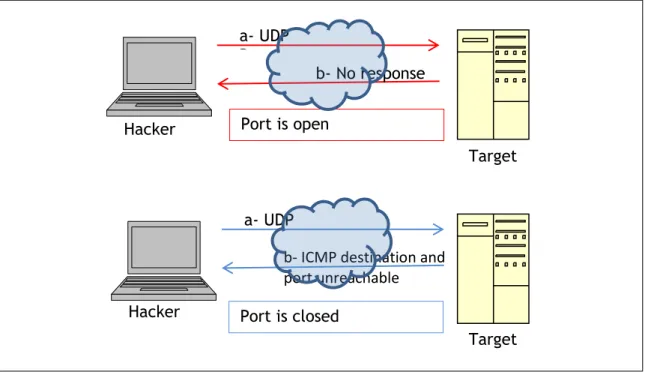
UDP scan works by sending a UDP packet to every targeted port. While most popular services on the Internet run over the TCP protocol, UDP services are widely deployed. DNS, SNMP, and DHCP (registered ports 53, 161/162, and 67/68) are three of the most common. Because UDP scanning is generally slower and more difficult than TCP, some security auditors ignore these ports. This is a mistake, as exploitable UDP services are quite common and attackers certainly don't ignore the whole protocol. A big challenge with UDP scanning is doing it quickly. Open and filtered ports rarely send any response. Closed ports are often an even bigger problem. They usually send
a- SYN b- SYN-ACK c- RST Hacker Target Port is open a- SYN b-RST Hacker Target Port is closed a- SYN b- SYN-ACK c- ACK Hacker Target Port is open a- SYN b- SYN-ACK Hacker Target Port is closed
17/93
back an ICMP port unreachable error. But unlike the RST packets sent by closed TCP ports in response to a SYN or connect scan, many hosts rate limit ICMP port unreachable messages by default. Linux and Solaris are particularly strict about this. For example, the Linux 2.4.20 kernel limits destination unreachable messages to one per second (in net/ipv4/ICMP.c).
Figure 3 shows the messages exchanger between Hacker and Target.
Figure 3: UDP scan
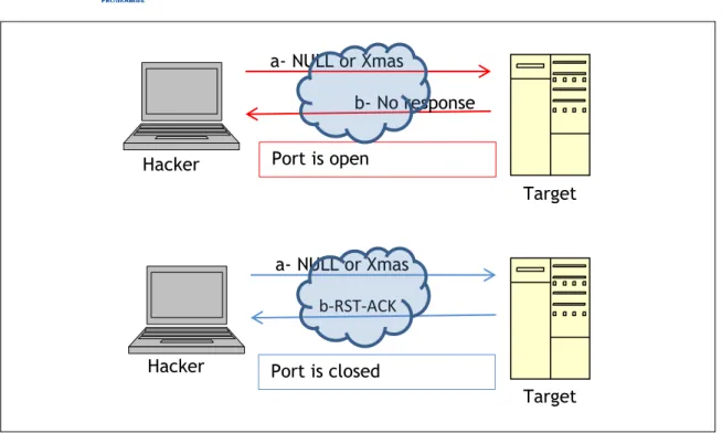
NULL scan: In a NULL scan a packet is sent to a TCP port with no flags set. In normal TCP communication, at least one bit—or flag—is set. In a NULL scan, however, no bits are set. RFC 793 states that if a TCP segment arrives with no flags set, the receiving host should drop the segment and send an RST.
Xmas scan: In Xmas scan, the attacker sends TCP packets with the following flags:
URG— Indicates that the data is urgent and should be processed immediately
PSH— Forces data to a buffer
FIN— Used when finishing a TCP session
The trick in this scan is not the purpose of these flags, but the fact that they are used together. A TCP connection should not be made with all three of these flags set. Usually, the host or network being scan returns a RST packet.
Figure 4 shows the messages exchanger between
Hacker and Target in the case of NULL or Xmas scan.
a- UDP Datagram b- No response Hacker Target Port is open a- UDP Datagram
b- ICMP destination and port unreachable Hacker
Figure 3: Target
18/93
Figure 4: TCP NULL and Xmas flags scan
Ping scan consists in sending an ECHO ping to a target (host discovery) or a network (network discovery). If a given address is alive, it returns an ICMP ECHO reply.
Figure 5 shows the messages exchanger between Hacker and Target.
Figure 5: ICMP scan
IP protocol scan allows you to determine which IP protocols (TCP, ICMP, IGMP, etc.) are supported by target machines. This isn't technically a port scan, since it cycles through IP protocol numbers rather than TCP or UDP port numbers.
4.1.2 Attacks
We selected some attacks, based on some articles describing attacks encountered in real life [4] [12]. Most attacks are DoS (Denial of Service) and DDoS (Distributed Denial of Service) attacks. The main goal of DoS and DDoS is to generate very huge flows of data, in order to generate dysfunction and or shutdowns of a selected target.
We have also some generic attacks, like FTP brute force cracking: the goal is to catch passwords used by applications like FTP.
1.1.1.1.
DDoS Attacks
2. Smurf a- NULL or Xmas scan b- No response Hacker Target Port is open a- NULL or Xmas scan b-RST-ACK Hacker Target Port is closed a- ICMP Echo_request b- ICMP Echo_reply Hacker Target If ICMP echo-reply from Target: Target is aliveIf ICMP echo-reply from router with destination/host unreachable: Target is not alive
19/93
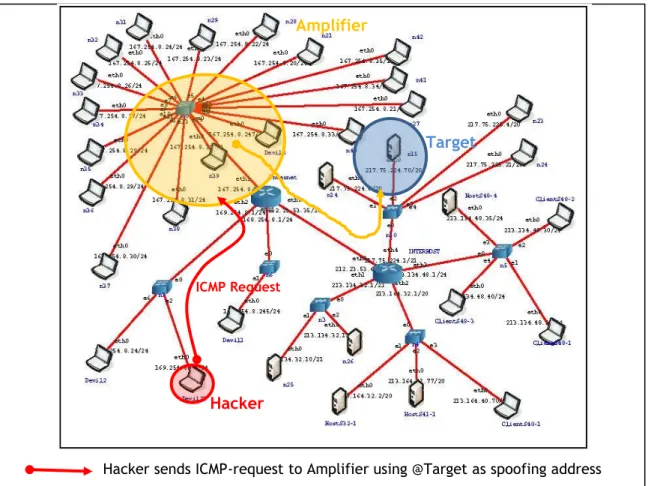
The Smurf Attack is a distributed denial-of-service attack where an attacker uses a set of amplifier hosts to exhaust the resource of a machine (the victim). The attacker sends a large numbers of Internet Control Message Protocol (ICMP) packets with the intended victim's spoofed source to a set of machines using an IP Broadcast address. These machines are the amplifiers. They will, by default, respond by sending a reply to the source IP address (which is the victim). If the number of machines on the network that receive and respond to these packets is very large, the victim's computer will be flooded with traffic. This can slow down the victim's computer to the point where it becomes impossible to work on. Figure 6 presents the architecture used to generate a Smurf attack.
Figure 6: Smurf attack
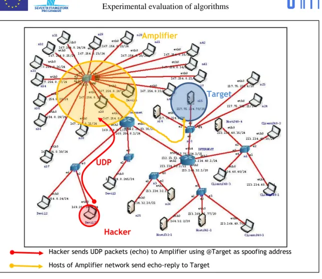
3. Fraggle
A Fraggle attack is a denial-of-service (DoS) attack that involves sending a large amount of spoofed UDP traffic to a router’s broadcast address within a network. It is very similar to a Smurf Attack, which uses spoofed ICMP traffic rather than UDP traffic to achieve the same goal. Given those routers (as of 1999) no longer forward packets directed at their broadcast addresses
Hacker sends ICMP-request to Amplifier using @Target as spoofing address Hosts of Amplifier network send ICMP-reply to Target
Hacker
Target Amplifier
20/93
Figure 7: Fraggle
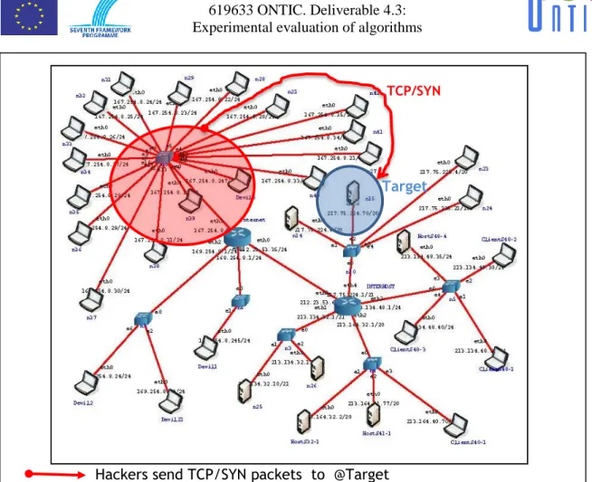
4. Syn DDoS
A SYN flood is a form of denial-of-service attack in which an attacker sends a succession
of SYN requests to a target's system in an attempt to consume enough server resources to make the system unresponsive to legitimate traffic. In the case of a Syn DDoS there are many
machines performing a SYN DoS targeting the same machine.
Hacke r
Target Amplifier
Hacker sends UDP packets (echo) to Amplifier using @Target as spoofing address Hosts of Amplifier network send echo-reply to Target
Hacker
Target Amplifier
21/93
Figure 8 – SYN DDoS attack
4.1.1.1.
DoS attacks
5. Syn FloodingA SYN flood is a form of denial-of-service attack in which an attacker sends a succession of SYN requests to a target's system in an attempt to consume enough server resources to make the system unresponsive to legitimate traffic
6. UDP flood
A UDP flood attack is a denial-of-service (DoS) attack using the User Datagram Protocol (UDP), a sessionless/connectionless computer networking protocol. Using UDP for denial-of-service attacks is not as straightforward as with the Transmission Control Protocol (TCP). However, a UDP flood attack can be initiated by sending a large number of UDP packets to random ports on a remote host.
7. Brute Force
The brute-force attack is still one of the most popular password cracking methods. It consists in trying many passwords or passphrases with the hope of eventually guessing correctly. The attacker systematically checks all possible passwords and passphrases until the correct one is found. It can be used for example to find the password used to secure SSH or FTP sessions.
4.2 Implementation
To generate the ground truth, we injected anomalies in real life network traces. These network traces come from the ONTS dataset collected in the context of the ONTIC project. This dataset is described in the deliverable D2.4 entitled “Provisioning subsystem. In this section, we
Hacke r
Target Amplifier
Hackers send TCP/SYN packets to @Target
Target TCP/SYN
22/93
describe how we select the ONTS traces where we inject the anomalies. Then, we describe the tools used for generating these anomalies. Finally, we present the obtained traces which form the ground truth.
4.3 Selection of the ONTS dataset
To generate the ground trace, a subset of the ONTS dataset is selected. The selected dataset must contain few anomalies which has to be clearly identified. Therefore, we select a small part of the ONTS dataset in order to be able to analyze it by hand.
4.3.1
Visualizing existing traces
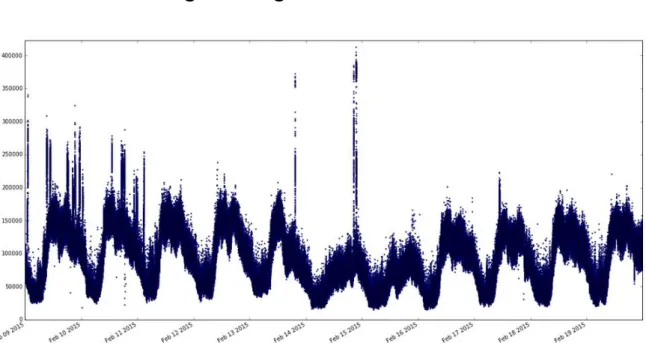
Figure 4: Time series which displays the number of packets per second in the ONTS dataset
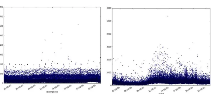
To select a subset of ONTS dataset which has few or no anomaly, we visualized 10 days of PCAP traces from the 9 to the 19 of February 2015. We created 17 temporal series of the data: the number of different destination ports, the number of different source ports, the number of different IP destinations, the number of RST packets, the number of FIN packets, the mean packet length, the number of ICMP reply, the number of unreachable ICMP packets, the number of ICMP echo packets, the number of time exceeded packets, the number of other types of ICMP packets, the number of SYN, the number of acknowledgments, the number of contention window reduction flag set to one, the number of URG packets, the number of push packets, the total number of packets. In order to process such a quantity of data, we use two servers of 28 cores each and process this data using PySpark and SparkSQL. We select PySpark because it allows sharing efficiently our findings using Jupyter, which is a python notebook. The Jupyter Notebook is a web application that allows creating and sharing documents that contain live code, equations, visualizations and explanatory text. We use also SparkSQL to query easily the data using SQL (Structured Query Language). Figure 4 displays time series: the number of packets in ONTS dataset during 10 days. One point represents one second of data. From this figure, the traces captured the 17 of February 2015 between 3PM and 4PM do not exhibit any peak and seems free from huge anomalies. Therefore, we select the dataset to inject anomalies. Figure 5 displays the number of RST packets and the number of ICMP echo packets per second for the selected day.
23/93
Figure 5: Number of RST packets and ICMP echo packets the 17th of February 2015
We then studied manually the selected PCAP and found that it contained anomalies. This study is possible as the selected PCAP is quite small. However, we cannot be totally confident that all the anomalies have been found. Using ORUNADA, we found two anomalies that we had not detected by hand. Table 1 shows a possible aggregation level with the associated key identifying the anomalous flow and the way we found the anomaly (by hand and/ or using our detector). Our solution identifies every anomaly detected manually plus two others. After investigation, the two anomalies found by our detector are pertinent and may be beneficial to a network administrator.
Table 1: Anomalies found manually with our detector
Classification of the
anomaly Description of the anomaly
Possible aggregation level and key for
identification Found
Network Scan UDP scan targeting a subnetwork IPSrc: 199.19.109.102 By hand + ORUNADA Network SYN scan IpSrc: 213.134.49.15 By hand + ORUNADA Network SYN scan IpSrc: 61.240.144.67 By hand + ORUNADA Network SYN scan IpSrc: 213.134.36.116 By hand + ORUNADA Port scan UDP Port scan of a machine P2P key:
119.81.198.93-217.75.228.214 By hand + ORUNADA Port scan of a machine P2P key: 213.134.39.11 - 10.10.150.14 ORUNADA
Large ICMP Large ICMP echo to one destination
P2P key:
213.164.33.194 -
8.8.8.8 By hand + ORUNADA
Large ICMP echo to one destination
P2P key:
195.22.14.100 -
213.134.54.133 By hand + ORUNADA
24/93
a network 213.134.32.141
Possible Attack Large Point Multi-Point ipDst key: 130.206.201.70 ORUNADA RST attack P2P key:
149.154.65.158-213.134.38.86 By hand + ORUNADA
4.4 Used Tools
In order to generate the ground truth we used many different tools: CORE, Nmap, Hping3, and Wireshark/Tcpdump. We used a network emulator to generate the network architecture. The network emulator allows us to build easily any network architecture and offers, therefore, a large flexibility. Furthermore and contrary to network simulators, a network emulator does not rely on any model to build the network. Therefore, it generates traces equivalent to those we could get with a real network platform.
4.4.1 Common Research Emulator (CORE)
Core [13] [14] [15] is an open source tool for emulating networks on one or more machines. CORE has been developed by a Network Technology research group that is part of the Boeing Research and Technology division. We use Core to emulate the Interhost network and the machines on the Internet. We have used the last version 4.8 (20150605).
4.4.2 Domain Information Groper (Dig)
Dig [16] is a flexible tool for interrogating DNS name servers. It performs DNS lookups and displays the answers that are returned from the name server(s) that were queried. Most DNS administrators use dig to troubleshoot DNS problems because of its flexibility, ease of use and clarity of output. Other lookup tools tend to have less functionality than dig. We have used dig 9.8.3-P1 for MacOS.
4.4.3 Network Mapper (Nmap)
We use Nmap [17] to generate every anomalies of type “Discovery”. Nmap ("Network Mapper") is a free and open source utility for network discovery and security. Nmap uses raw IP packets to determine what hosts are available on the network, what services (application name and version) those hosts are offering, what operating systems (and OS versions) they are running, what type of packet filters/firewalls are in use, and dozens of other characteristics. We have used Nmap 6.40 for Ubuntu 14.04 LTS and Nmap 7.01 for Ubuntu 16.04 LTS.
4.4.4 Hping3
We use Hping3 [18] to generate some of the attacks. Hping3 is a network tool able to send custom TCP/IP packets and to display target replies like ping program does with ICMP replies. Hping3 handle fragmentation, arbitrary packets body and size and can be used to transfer files encapsulated under supported protocols. We used hping3 3.0.0-alpha-2 for Ubuntu 16.04 LTS.
4.4.5 Nping
Nping [19] is an open source tool for network packet generation, response analysis and response time measurement. Nping can generate network packets for a wide range of protocols, allowing users full control over protocol headers. While Nping can be used as a simple ping utility to detect active hosts, it can also be used as a raw packet generator for network stack stress testing, ARP poisoning, Denial of Service attacks, route tracing, etc. We used nping 0.7.01 for Ubuntu 16.04 LTS.
25/93
4.4.6 Hydra
Hydra [20] is a parallelized login cracker which supports numerous protocols to attack. It is very fast and flexible, and new modules are easy to add. This tool makes it possible for researchers and security consultants to show how easy it would be to gain unauthorized access to a system remotely. We used Hydra v8.1 for Ubuntu 16.04 LTS.
4.4.7 Ncrack
Ncrack [21] is a high-speed network authentication cracking tool. Ncrack's features include a very flexible interface granting the user full control of network operations, allowing for very sophisticated bruteforcing attacks, timing templates for ease of use, runtime interaction similar to Nmap's and many more. Protocols supported include RDP, SSH, HTTP(S), SMB, POP3(S), VNC, FTP, SIP, Redis, PostgreSQL, MySQL, and Telnet. We used Ncrack 0.5 for Ubuntu 16.04 LTS.
4.4.8 Wireshark/Tcpdump
Wireshark [22] and tcdump were used to collect the traffic on CORE, to modify the time of the generated attacks so that they are consistent with the ONTS dataset and to check the generated ground truth. Tcpdump is a common packet analyzer that runs under the command line. It allows the user to display TCP/IP and other packets being transmitted or received over a network to which the computer is attached. Distributed under the BSD license, Tcpdump is free software. It offers many features to analyze, filter and modify packet traces. As Tcpdump, Wireshark is a free and open source packet analyzer. It is used for network troubleshooting, analysis, software and communications protocol development. We mainly use Wireshak for its graphical user interface and Tcpdump for its speed and lightness. We used Wireshark 2.0.x and Tcpdump 4.7.4 for Ubuntu 16.04 LTS.
4.5 Traces generation
To generate the anomalies, we built different network architecture using CORE. These networks are very close to the one used by Interhost. Interhost is a subsidiary of Satec. The ONTS dataset was collected at the border of the Interhost network. This border is represented in Figure 6 and Figure 7 by the router named Interhost and the four subnetworks of Interhost by the 4 branches directly connected to the Interhost router.
4.5.1 Discovery anomalies
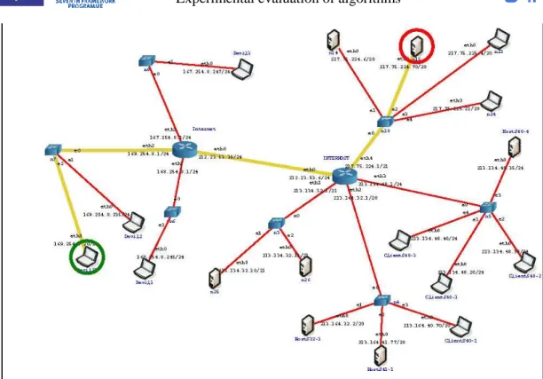
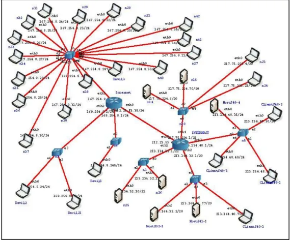
Figure 8 describes the network built with Core and used to generate the anomalies of type “Discovery anomalies”. For every anomaly of type “discovery anomalies” we use the same attacker (Devil21 with a green circle on the figure) and the same target which represents a SATEC machine (n15 with a red circle on the figure).
The commands used to generate these anomalies and the obtained anomalies description is described in details in Annex A.
26/93
Figure 6: Network used to generate anomalies of type "Discovery anomalies"
4.5.2 Attacks
Figure 7 describes the network used to generate the attacks on CORE. Compared to the previous network described in Figure 6, a high number of machines are added (only some of them are represented in the figure). They are used for amplification attacks like the Smurf and Fraggle attack.
The commands used to generate these anomalies and the obtained traces are described in details in Annex B.
27/93
Figure 7: Network used to generate the attacks on CORE
Finally, the most important anomalies generated in this ground truth are presented in Table 2. This table displays the tool used to generate the anomaly, the mean byte rate of the anomaly, the size of the traces once the anomaly injected. A more detailed description of the anomalies generated and the obtained traces is available in Annex C.
Table 2: Descriptions of the some anomalies Tool used Anomaly Generated file :
fusion_SATEC_*.pcap Mean Byte rate Size file GBytes Discovery anomalies
Nmap Scan OS,
services and open ports for 1 target
scan_os_host 51 MBps 1.425
Nmap Scan OS,
services and open ports for sub-network
scan_os_network 51 MBps 1.428
Ports scans
Nmap TCP SYN scan TCP_SYN_p5T000 51 MBps 1.426
Nmap TCP CONNECT
scan TCP_Connect_p5000 51 MBps 1.433
Nmap UDP scan UDP_scan_T5 51 MBps 1.426
Nmap NULL scan NULL_scan_T4 51 MBps 1.425
28/93
Network scans
Nmap Ping scan Ping_scan_T4 51 MBps 1.426
Nmap IP Protocol
scan IP_proto_scan_T4 51 MBps 1.427
Attacks
DDoS
hping3 smurf smurf_hping3 15.107
Nping fraggle fraggle_nping 58.065
hping3 Syn flooding synflood_ddos_hping3 60MBps 4.233
DoS
hping3 Syn flooding synflood_dos_hping3 64MBps 5.330
Nping UDP flood udpflood_nping 63MBps 5.192
BruteForce
Ncrack BruteForce brute_force_ncrack_rockyou 52 MBps 1.922
4.6 Ground truth use and dissemination
The generated ground truth can be used to validate any unsupervised network anomaly detector. Compared to existing ground truth in the field, we claim that the ONTS ground truth has many advantages:
8. It is realistic. Indeed, this ground truth is based on real network traces and the injected anomalies were generated taking in considerations the characteristics (architecture, IP addresses, nb of routers, etc) of Interhost network. Interhost network is the network where the real traces were collected. Therefore, the generated anomalies are consistent with the ONTS dataset.
9. It is exhaustive in its labels. As we manually check the traces, we are quite confident on the fact that most of the anomalies are labelled in the traces.
10. Rich in the number of anomalies generated.
This ground will be made available on demand. We hope that it will be valuable for many persons working in the field of unsupervised network anomaly detection.
29/93
5 Network
Anomaly
and
Intrusion
Detection
Algorithms
With the booming in the number of network attacks, the problem of network anomaly detection has received increasing attention over the last decades. However, current network anomaly detectors are still unable to deal with zero days attack or new network behaviors and consequently to protect efficiently a network. Indeed, existing solutions are mainly knowledge-based and this knowledge must be continuously updated to protect the network. However building signatures or new normal profiles to feed these detectors take time and money. As a result, current detectors often leave the network badly protected.
To overcome these issues, a new generation of detectors has emerged which takes benefit of intelligent techniques which automatically learns from data and allows bypassing the strenuous human input: unsupervised network anomaly detectors. These detectors aim at detecting network anomalies in an unsupervised way, i.e. without any previous knowledge on the anomalies. They mainly rely on one main assumption [23] [24]:
“Intrusive activities represent a minority of the whole traffic and possess different patterns from the majority of the network activities.”
A network anomaly can be defined as a rare flow whose pattern is different from most of other flows. They are mainly induced by [25]:
Network failures and performance problems like server.
Network failures, transient congestions, broadcast storms.
Attacks like DOS, DDOS, worms, brute force attacks.
Thus, unsupervised network anomaly detectors exploit data mining algorithms to identify flows which have rare patterns and are thus anomalous. A state of the art on network anomaly detection can be found in section 6.1 of the deliverable D4.1. Existing unsupervised network anomaly detectors mainly suffer from four issues:
1. Complexity issue: a high complexity which prevents them from being real time. We define an application as real time if it is able to process the data as soon as it arrives. To overcome this limitation some detectors only process sampled network data, implying that the malicious traffic may not be processed and detected [26].
2. Latency issue due to large time slots to collect the traffic. Indeed, the network traffic is usually collected in consecutive equally sized large time-slots on one or many network links. The length of a time-slot has to be sufficiently large so that unsupervised network anomaly detectors gather enough packets to learn flows patterns. As a result, a substantial period of time may elapse between an anomaly occurrence and the process of the anomaly [25].
3. Detection issue due to a poor description of the incoming traffic. According to the granularity and the aggregation level used to describe the incoming traffic, a detector does not detect the same anomalies in the data. The way the incoming data is described may have a huge impact on the capability of the detector to identify anomalies. Many detectors due to their high complexity only describe the traffic using statistics and have a coarse view of the data [7]. Some other detectors use only one aggregation level to create flows and compute statistics for each flow [27]. In this case, they only have one representation of the data and may not be able to detect many different types of anomaly. We claim that it is important to describe the traffic using different aggregation levels in order to spot most attacks.
30/93
4. Detection issue due to a lack of temporal information. Most detectors only consider the information gathered at a time slot to decide whether there is an anomaly or not. However, it may be important to consider the evolution of the data and add temporal information. Indeed, a flow that stands out from the others at a time t should not be considered as an anomaly if it is always “different”. It may then be just a flow induced by a special server on the Internet like the google DNS server.
The unsupervised network anomaly detector presented in this section and named Streaming ORUNADA Unsupervised Network Anomaly detector tackles these four different issues.
ORUNADA is an unsupervised network anomaly detector presented in deliverable 4.2 which aims at detecting in real time and in a continuous way the anomalies on a network link. ORUNADA deals with the first and second issue encountered in actual unsupervised network anomaly detectors presented above. To overcome these issues, it relies on a discrete time sliding window and an incremental grid clustering algorithm. The discrete time sliding window allows a continuous detection of the anomaly whereas the incremental grid clustering algorithm a low computational complexity of our solution. The validation of ORUNADA shows that it could detect online in less than a second an anomaly after its occurrence on a high rate network link (the evaluation was performed on the ONTS dataset).
In order to solve the issues 3 and 4 described above, we propose an improved version of ORUNADA named Streaming-ORUNADA. This later considers multi aggregation level in order to spot more anomalies and the evolution of the feature space over time. It is inspired from streaming clustering algorithms as it track clusters and outliers over time, hence the name of this new detector Streaming-ORUNADA. For the implementation of Streaming-ORUNADA, we take advantage of an existing cluster computing framework Spark Streaming, therefore the implementation is called Spark-Streaming-ORUNADA and is available on the ontic gitlab at the following address https://gitlab.com/ontic/wp5-laascnrs-orunada.
This section starts with a formal definition of an anomaly. Then, it describes in three steps our solution: the data preprocessing step, the incremental clustering step, and the post-processing step. Finally, the validation of our solution using the ground truth presented in section 4 is presented. Details about the implementation of our algorithm on Spark, the Google Dataproc platform used for the validation and the platform parameterization is given in the following section, i.e. section 6 of the deliverable.
5.1 Definition of an anomaly
An anomaly is usually defined as a flow which is different from the other flows. However, this definition is quite vague, that is why we define, in the following, more precisely what we consider as an anomaly in our solution.
First, we make some assumptions about the nature of the anomalies that a network administrator wants to be aware of and how these anomalies should appear using clustering techniques. First, let’s introduce some concepts of clustering techniques applied to network anomaly. Usually the data to partition is represented by a matrix where each line represents a flow and each column a statistic. This matrix is called the space or feature space. Each flow represents a point of the space and the coordinates of the point are the statistics of the flow. The set of points is the space. A clustering algorithm applied on a space (the data matrix) output a partition of the feature space. It identifies clusters (group of points which are close to each other according to a given distance function) and outliers. An outlier is a point which is isolated. The following figure shows the result of a clustering algorithm (a partition of the feature space): two clusters and two outliers can be clearly identified.
31/93
Figure 8: Partition of a space with two clusters and two outliers
In the following we assume, that any network administrator wants to be aware of rare events going on in the network, this event should be rare not only at a given time, but also considering the traffic history (see issue 4 of current unsupervised network anomaly detector presents in section 5). We define a rare event as either:
A flow different from the others which was not different in the past. Indeed, if a flow is always rare in the same way (the flow set of statistic stay the same over time), this latter may not interest the network administrator. It may be just a flow induced by a particular server on the network, like the flow induced by the google DNS server. Such an anomaly may appear as a new outlier in a space.
A flow different from the others whose statistics suddenly change. Indeed a flow which is always different from the other may not be considered as an anomaly. However, if its statistics change suddenly, it means that something “special” like an attack or a failure is happening on the server. Therefore, such a flow needs to be considered as an anomaly. Such a flow may appear as an outlier shifting suddenly in the space.
A set of flows which appear or disappear suddenly. This set of flows can be, for example, induced by a DDOS. For example, when a server is under a DDOS the number of flows targeting this network may increase in a significant way. Therefore, the cluster representing the set of flows targeting this network may increase drastically. Such an anomaly may appear as a change (increase or decrease) in the size of a cluster or as the disappearance or appearance of a new cluster.
By using clustering techniques, these rare and interesting events for a network administrator can be defined in a formal way. To define them, three new parameters (in addition to the clustering parameters) are considered:
1. Thist. This parameter represents the length of the historic in second that is considered. A
cluster or an outlier is considered as new in a space if it was not present in this space during the This last seconds. This value should be set according to the capacity of
memory of the machine running the detector. It also should not be too long in order to adapt to the network traffic changes.
2. Nclust. This parameter is a threshold, when the number of points of a cluster change (it
increases or decreases of at least Nclust points) the cluster (and all the flows that it
contains) can be considered as an outlier.
3. . This parameter is a threshold, if a point (flow) moves of a least a distance during the This last seconds. We consider that the flow statistics changed.
We define formally an anomaly as either:
1. A flow which is an outlier in a space S and has never been detected as an outlier in S before (i.e. during the last This seconds).
2. A flow detected as an outlier in a space which shifted by a distance of at least during the This last seconds.
3. A cluster C which disappears
32/93
5. A cluster C whose size changes of at least Nclust points during the This last seconds.
5.2 Data preprocessing
Before applying any unsupervised network anomaly detectors, the network traces must be collected on the network link in time slots. To collect the traffic, our solution relies on a discrete time sliding window. This window slides every micro-slot. At each slide, the traffic must then be processed in order to compute N data matrix X, one for each aggregation level. Each data matrix represents a different summary of the incoming traffic.
To collect the traffic, our solution relies on a discrete time sliding window. This window allows generating in a continuous manner N data matrix by micro time slot and thus, to detect in continuous the anomalies. Furthermore, each data matrix must be normalized. Many data mining techniques used to detect anomalies are sensitive to features that have different range of values. Indeed, features with high values often hide features with lower values. Therefore, it is very important to normalize the data. Furthermore, this normalization needs to evolve with the traffic characteristics.
First, this subsection describes the functioning of the discrete sliding window. It then presents the N different aggregation levels and their associated features. Finally, it describes an adaptive normalization method.
33/93
6 The discrete time sliding window
The detection is usually performed on network traffic collected in large time-slots implying long period of time between an anomaly occurrence and its detection. To overcome this issue, we propose to use a discrete time-sliding window in association with an unsupervised network anomaly detector. The proposed method is generic: any sufficiently fast and efficient detector can benefit from the proposed solution to reach continuous and real-time detection.
The traffic has to be collected in large time-slots of length ∆T in order to gather enough packets to catch flows patterns. Evaluations presented in [22] showed that time-slots of 15 seconds give good results in terms of detection performance (TPR and FPR).
Collected traffic is then aggregated into flows using N different aggregation levels. In the following, we decide to use 7 different aggregation levels that will be described later. Therefore, our solution outputs 7 different data matrices .
Every flow is described by a set of features (these features are different according to the aggregation level used to generate the flow) stored in a vector. All the vectors generated with the same aggregation level are then concatenated in a normalized matrix , is the aggregation level. The network anomaly detector processes independently every data matrix. The process of consecutive time-slots is illustrated in Figure 9.
Figure 9: Computation of the N feature spaces at the end of every time slot (or window) of length
∆T
To avoid that attacks damage the network, network anomalies have to be rapidly detected. To speed up the anomaly detection, we propose to update the N feature spaces and launch the detection in a near continuous way, i.e. every micro-slot of length δt seconds. However, if a feature space is computed with only the network traffic contained in a micro-slot, it may not contain enough information for the detectors to identify flows patterns and thus anomalies. To solve this issue, we use a discrete time sliding window of length ∆T. The time window slides every micro-slot of length δt. When it slides, the feature space is updated. The feature space is the summary of the network traffic collected during the current time-window (see Figure 10).
34/93
A discrete time-sliding window is made up of M micro-slots with . To speed-up the computation of a feature space , the sliding window associates to each of its M micro-slots a micro-feature space . Each micro-feature space is computed with the packets contained in its micro-slot.
For every aggregation level, the current window stores M micro-feature spaces in a FIFO queue Q = denotes the micro-feature space computed for one aggregation level with the packets contained in the newest micro-slot and in the oldest. For a given aggregation level, when the window slides a new feature space denoted can be computed as follows:
where is the previous feature space and the new micro-feature space. Finally, the FIFO queue is updated, is added to the FIFO queue and, is removed. To benefit from these feature space updates, we devise a detector algorithm capable of detecting in continuous anomalies. To reach this goal this detector is based on a distributed algorithm and each parallel task is based on an incremental grid clustering step which has a low complexity.
6.1.1 Description of the aggregation levels and their associated features
Incoming packets are collected in consecutive time bins ∆T and aggregated into flows according to different aggregation levels. An aggregation level can be described by a filter and a flow aggregation key. Incoming packets are first filtered and then grouped into flows according to a flow aggregation key. A flow aggregation key specifies a set of fields to inspect in a packet. Packets with similar values for these fields are aggregated into flows. Each flow is then described by a set of attributes or features. Anomalies identified by a detector may be different according to the aggregation level used. Therefore, we apply different aggregation level to the incoming traffic. For every aggregation level at the end of every time bin, it outputs a set of flows forming a feature space . We use seven different aggregation levels. Every aggregation level is described in Table 3. This table displays for every level its filter, its flow aggregation key and the features used to describe a flow. To compute a feature space, they consider every packet of flows in the current time slot (window). Some features are based on the entropy, as previous studies showed that the distribution of some traffic features may reveal anomalies [7]. For example, for the aggregation level at the IP source, we compute the entropy of the source and destination ports and the entropy of the IP destinations. A high entropy of the IP destinations and a low entropy of the source ports imply that the distribution of the source ports is very sparse while the distribution of the IP destinations is very dense and this may reveal a port scan.
Table 3: Description of the different aggregation levels and associated features
Aggregation
level
Filter
Aggregation
Key
Features
Number of
Features
1 TCPpackets TCP socket pair nbPacketsIP1, nbPacketsIP2, nbSyn, nbAck, nbCwr, nbUrg, nbPush, nbRst, nbFin, bytesIP1, bytesIP2, land, nbChristmasTree, nbMoreFrag
14
2 UDP
packets UDP socket pair nbPacketsIP1, nbPacketsIP2, bytesIP1, bytesIP1, land, nbMoreFrag 6
3 ICMP
packets pair of IP addresses nbPacketsIP1, nbPacketsIP2, bytesIP1, bytesIP2, land, nbReply, nbEcho, nbOther, nbRedirect, nbUnreach, nbTimeExceeded, nbMoreFrag
12
4 No pair of IP
addresses
nbPacketsIP1, nbPacketsIP2, nbSyn, nbAck, nbCwr, nbUrg, nbPush, nbRst, nbFin, bytesIP1, bytesIP2, land, nbChristmasTree, nbTimeExceeded,
35/93
nbUnreach, nbEcho, nbRedirect, nbReply, entPortIP1, entPortIP2,
nbICMPOther, nbMoreFrag,
nbPacketsTCP, nbPacketsUDP
5 No IP source nbPackets, nbSyn, nbAck, nbCwr,
nbUrg, nbPush, nbRst, nbFin, bytes,
nbland, nbChristmasTree,
nbTimeExceeded, nbUnreach, nbEcho, nbRedirect, nbReply, entPortSrc, entPortDst, nbICMPOther, nbMoreFrag,
nbPacketsTCP, nbPacketsUDP,
entIPSrc, simIPSrc,
24
6 No IP
destination
nbPackets, nbSyn, nbAck, nbCwr, nbUrg, nbPush, nbRst, nbFin, bytes,
nbland, nbChristmasTree,
nbTimeExceeded, nbUnreach, nbEcho, nbRedirect, nbReply, entPortSrc, entPortDst, nbICMPOther, nbMoreFrag,
nbPacketsTCP, nbPacketsUDP,
entIPSrc, simIPSrc
24
7 No No nbPacketsIP1, nbPacketsIP2, nbSyn,
nbAck, nbCwr, nbUrg, nbPush, nbRst, nbFin, bytesIP1, bytesIP2, land, nbChristmasTree, nbTimeExceeded, nbUnreach, nbEcho, nbRedirect, nbReply,entPortIP1, entPortIP2,
nbICMPOther, nbMoreFrag,
nbPacketsTCP, nbPacketsUDP
24
We also use the TCP socket pair and the UDP socket pair as aggregation levels. A socket pair is a unique 4-tuple consisting of source and destination IP addresses and port numbers.
Packets are collected on a large network link in consecutive time slots. For every aggregation level except for the aggregation level 7, our solution computes a large set of flows at every time slot. This set is assumed to be large as our solution is applied on the traffic captured on a large network link. However, for the aggregation level 7, only one flow is computed at each time slot. This unique flow summarizes the behavior of the entire link. Therefore, our solution is slightly different when it processes flows computed at the aggregation level 1, 2, 3, 4, 5, 6 and glows generated with the aggregation level 7.
For the aggregation level 1, 2, 3, 4, 5, 6, flows computed during a time slot are directly partitioned using the solution presented thereafter. However, for the aggregation level 7, a certain number of time-slots must pass to collect enough flow (one per time slot) to partition them. Once a set of N (with N large) flows are collected they can be partitioned.
6.1.2 Feature space normalization
In the following, data for each aggregation level is represented by a matrix of size where each row represents a point (or flow in our case) and each column a feature (or dimension). To apply data mining techniques, data features must be comparable and therefore have the same common domain. Data normalization refers to the creation of shifted and scaled versions of every feature. It allows mapping the features values via a transformation function in a common domain. After normalization, features values can be compared. As explained in [28], normalization may be sensitive to outliers and should be removed for the