Laboratory Experiments of Ice Scour Processes

(1)

https://doi.org/10.4224/12328892

READ THESE TERMS AND CONDITIONS CAREFULLY BEFORE USING THIS WEBSITE.

https://nrc-publications.canada.ca/eng/copyright

Vous avez des questions? Nous pouvons vous aider. Pour communiquer directement avec un auteur, consultez la première page de la revue dans laquelle son article a été publié afin de trouver ses coordonnées. Si vous n’arrivez pas à les repérer, communiquez avec nous à PublicationsArchive-ArchivesPublications@nrc-cnrc.gc.ca.

Questions? Contact the NRC Publications Archive team at

PublicationsArchive-ArchivesPublications@nrc-cnrc.gc.ca. If you wish to email the authors directly, please see the first page of the publication for their contact information.

Archives des publications du CNRC

For the publisher’s version, please access the DOI link below./ Pour consulter la version de l’éditeur, utilisez le lien DOI ci-dessous.

Access and use of this website and the material on it are subject to the Terms and Conditions set forth at

Laboratory Experiments of Ice Scour Processes

Barker, Anne; Timco, Garry

https://publications-cnrc.canada.ca/fra/droits

L’accès à ce site Web et l’utilisation de son contenu sont assujettis aux conditions présentées dans le site LISEZ CES CONDITIONS ATTENTIVEMENT AVANT D’UTILISER CE SITE WEB.

NRC Publications Record / Notice d'Archives des publications de CNRC:

https://nrc-publications.canada.ca/eng/view/object/?id=b040b438-9a61-40e6-b60c-202da0c3e7ac https://publications-cnrc.canada.ca/fra/voir/objet/?id=b040b438-9a61-40e6-b60c-202da0c3e7ac

(2)

Laboratory Experiments of Ice Scour Processes

Anne Barker and Garry Timco Canadian Hydraulics Centre National Research Council of Canada

Ottawa, Ont. K1A 0R6 Canada

Technical Report CHC-TR-004

PERD/CHC Report 31-28

(3)

(4)

ABSTRACT

A laboratory program has been carried out to measure the loads and seabed response due to an ice block scouring a representative seabed. The results are meant to provide experimental data for a numerical model that can be used for predicting scour depths and pressures in the Grand Banks region. Fourteen tests were performed with a variety of seabed types that are representative of the Grand Banks region. Blocks of freshwater ice were used to scour the seabed. The scouring loads and resulting trenches were measured. This report provides a description of the test arrangement and the experimental results.

(5)

2.6.2 Scour Profiles ...17 3. RESULTS ...19 3.1 Test #1 – Scour_001 ...19 3.2 Test #2 – Scour_002 ...23 3.3 Test #3 – Scour_003 ...23 3.4 Test #4 – Scour_004 ...23 3.5 Test #5 – Scour_005 ...24 3.6 Test #6 – Scour_006 ...24 3.7 Test #7 – Scour_007 ...25 3.8 Test #8 – Scour_008 ...25 3.9 Test #9 – Scour_009 ...25 3.10 Test #10 – Scour_010 ...25 3.11 Test #11 – Scour_011 ...25 3.12 Test #12 – Scour_012 ...26 3.13 Test #13 – Scour_013 ...26 3.14 Test #14 – Scour_014 ...26 4. ANALYSIS ...27 4.1 Scour Profiles ...27 4.2 Force Data ...28 4.3 Observational Data ...30 4.4 Ice Failure ...32 5. SUMMARY...33 6. ACKNOWLEDGEMENTS ...34 7. REFERENCES...35 APPENDIX ...1

(6)

TABLE OF FIGURES

Figure 1 Photo of typical Grand Banks sand and gravel seabed (Sonnichsen,

2001)... 3

Figure 2 Sand chosen to represent Hibernia Sand Formation/Adolphus Sand (Davies, 2002)... 3

Figure 3 9.5mm gravel chosen to represent the Hibernia Gravel Formation (Davies, 2002)... 4

Figure 4 Seabed preparation – gravel on left side, sand on right... 5

Figure 5 Sand with gravel overlay channel... 6

Figure 6 Cut view of sand with gravel overlay ... 7

Figure 7 Crushing ice for models ... 8

Figure 8 “Filtering” ice for models, through a 0.02 m screen... 8

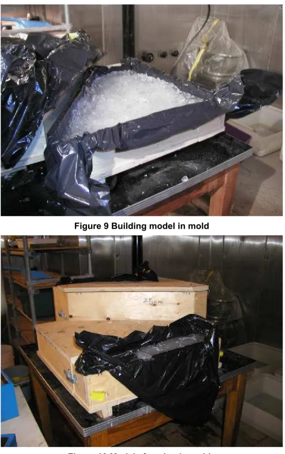
Figure 9 Building model in mold ... 9

Figure 10 Models freezing in molds ... 9

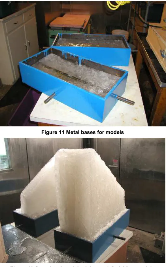
Figure 11 Metal bases for models ... 10

Figure 12 Completed models, 0.1 m on left, 0.25 m on right ... 10

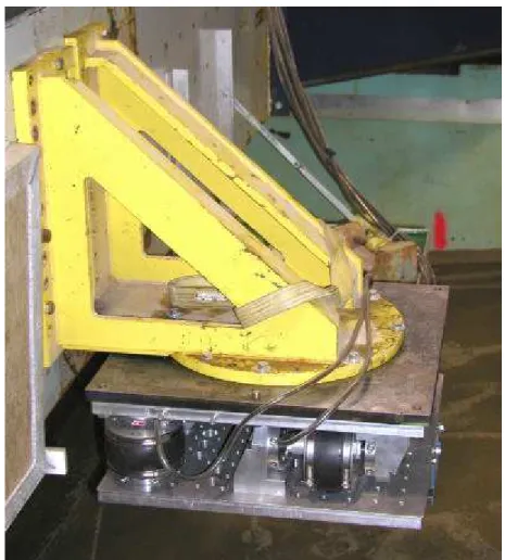
Figure 13 Installing the 0.1 m model below the dynamometer... 11

Figure 14 6-component dynamometer underneath mounting bracket and plate 12 Figure 15 Pressure transducer layout ... 12

Figure 16 Pore pressure transducers mounted on stainless steel rod ... 13

Figure 17 Schematic of ice tank set-up ... 14

Figure 18 Schematic of model placement... 14

Figure 19 Test set-up showing location of video camera ... 16

Figure 20 Profiling the scour track... 18

Figure 21 Summary of x- and z- forces measured on the dynamometer for Scour_001... 20

Figure 22 Summary of pressure forces measured for Scour_001 ... 21

Figure 23 Profiles measured for Scour_001 ... 22

Figure 24 Scour_002, 0.1 m scour depth ... 22

Figure 25 Scour_002, 0.25 m scour depth ... 23

Figure 26 Maximum pressures recorded for tests Scour_004, Scour_007, Scour_008... 24

Figure 27 Photograph of two of the drained channels after the second series of three tests. ... 27

Figure 28 Ratio of backfill area divided by original fill area for all tests ... 28

Figure 29 Measured versus predicted forces for each seabed type ... 29

Figure 30 Measured versus predicted forces for all data combined... 30

Figure 31 Ice model #3, initially 0.1 m wide over the entire length, before and after testing ... 31

(7)

(8)

LABORATORY EXPERIMENTS OF ICE SCOUR PROCESSES

1. INTRODUCTION

The presence of icebergs is one of the main challenges facing the full development of the petroleum resources in the Grand Banks regions of Canada. In addition to being a threat to fixed (GBS) and floating (FPSO) structures, they also have a profound influence on seabed facilities and pipeline transportation systems for offshore natural gas. Icebergs have been observed to interact with the sea floor creating scour features. The nature, depth, width and zone of influence of these scours are the major factors affecting feasibility of subsea facilities and seabed pipelines. Although there is knowledge of the depth of existing scours (Sonnichsen and King, 2001), there is limited knowledge of the factors that control the depth and the loads associated with the scouring process. There have been a number of previous laboratory studies of iceberg scouring (see Clark et al., (1998) for a recent review). These can be classified into two different types – (1) physical tests using rigid indentors in a laboratory flume that is filled with a geotechnical material (Poorooshasb, 1989; Gulf Canada Ltd. and Golder Associates Ltd., 1989; Poorooshasb and Clark, 1990; Abdelnour, R. and Lapp, D., 1980), and (2) centrifuge experiments of scouring processes (Woodworth-Lynas et al., 1995; Phillips, personal communication). The first approach can provide good information on the scouring process, but it is difficult to scale these results to the full-scale situation using conventional modeling laws. The centrifuge approach has distinct advantages in data analysis, but these experiments are costly and difficult since they are performed with relatively small models. In the present tests, the first approach has been used. In contrast to previous tests of this type that used steel indentors for scouring, the present tests used large blocks of ice for scouring the seabed. This allowed potential ice failure during the tests. Prior to the tests, Sonnichsen and King (2001) carried out a study to document the characteristics of the seabed of the Grand Banks region. These characteristics were used in these tests. The data was intended to supply information for a numerical model of the ice scouring process.

(9)

2. MODELLING ICE SCOUR

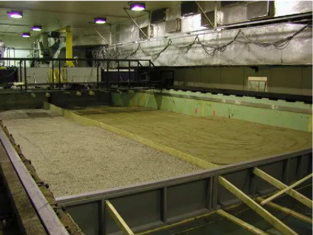
2.1 Test Facility

The tests were performed in the ice tank at the NRC Canadian Hydraulics Centre in Ottawa (Pratte and Timco, 1981). The tank is 21 m long by 7 m wide and 1.2 m deep, and is housed in a large insulated room that can be cooled down to an air temperature of -20°C. A carriage that can travel the length of the tank spans the tank. The carriage is driven through two helical-cut rack and pinion gears, and is designed for loads up to 50 kN with a speed range from 0.003 to 0.65 m/s. In the usual test procedure, the structure is mounted through the compliance simulator to the front face of the carriage and the carriage is driven along the tank, simulating the interaction process. An additional service carriage also spans the tank. For these tests, the service carriage was clamped to the main carriage, and was thus driven along the tank ahead of the main carriage. During a test, the output from the instrumentation was sampled, digitized and stored for subsequent analysis and computation.

2.2 Seabed

2.2.1 Soil Selection

A photograph of a typical Grand Banks sand and gravel seabed is shown in Figure 1. The photo was taken in shallower water (between 100 m and 110 m water depth) where a gravel lag is present. It was desirable to match these conditions as much as possible for the test program.

Soil selection was contracted to Dr. Michael Davies, of Pacific International Engineering. His report recommended the following soils for the test program:

• “A coarse, well-graded sand representative of the Hibernia Sand Formation and selected to give friction angles compatible with those anticipated for the Adolphus Sand Formation.” (Figure 2)

• “A clear, well-graded fine gravel representative of the Hibernia Gravel Formation.” (Figure 3)

• “A bed of the coarse sand overlain by the fine gravel to represent a typical armoured bed” (Davies, 2002).

(10)

Figure 1 Photo of typical Grand Banks sand and gravel seabed (Sonnichsen, 2001)

Figure 2 Sand chosen to represent Hibernia Sand Formation/Adolphus Sand (Davies, 2002)

(11)

Figure 3 9.5mm gravel chosen to represent the Hibernia Gravel Formation (Davies, 2002)

The sand that was selected is a well-graded, medium-coarse sand, with characteristic sizes, from sieve analysis performed at CHC, of:

D90=1.8mm, D50=0.65mm, D10=0.25mm.

The gravel that was chosen is a 9.5 mm, well-graded, fine gravel, with characteristic sizes of:

D90=14mm, D50=7mm, D10=2mm, Cu=D60/D10=8.5/2=4.25.

Both the sand and the gravel were very clean in order to avoid turbidity in the water. Davies (2002) carried out a quick assessment to determine whether the selected materials were compatible for tests of sand overlying the gravel. He found that Terzaghi’s filter criteria were satisfied, and therefore that “the soils are suitable for a test where gravel is placed over top of the sand to replicate the bed armouring condition which would be common in the Hibernia Sand and Gravel formation” (ibid.).

Direct simple shear tests of the sand were performed by Jacques Whitford and Associates (ibid.). The samples were tested at three dry densities and sheared at two strain rates. The confining stress was 5 kPa, which would correspond “to the confining stress which would exist under about 0.3m of soil” (ibid.), in order to approximate the test conditions in the ice tank at CHC. The resultant peak shearing resistance angles ranged from 44° to 62°, with residual angles of shearing resistance ranging between 34° and 42°(ibid.).

In addition, three in situ bulk density tests were performed after the second series of tests, after the test basin was drained. Tests were performed using a

(12)

thin-walled sampling tube (ring) with a 0.05 m diameter, that was driven into the seabed to a set depth. The collected material was weighed, dried and re-weighed. These tests gave an average dry density value of approximately 1816 kg/m³.

2.2.2 Preparation

The sand and gravel selected for the test series were placed in the ice tank by a loader in the dry. A plywood divider wall was constructed down the length of the tank in order to separate the sand and the gravel sections (Figure 4). The seabed material was placed in approximately 0.15 m lifts. As each lift was placed, some water was added to facilitate packing. Packing was performed on each lift using a vibratory plate compactor.

Figure 4 Seabed preparation – gravel on left side, sand on right

As two scouring depths were desired for the test series, the seabed materials were placed at two heights along the length of the channel. The first level was built up to 0.35 m from the bottom of the ice tank, the second at 0.5 m, with a gradual transition over 1 m between the two. This resulted in scouring depths of 0.1 m and 0.25 m respectively as the ice passed through the materials. The run length for each height was approximately 5 m.

Once the material had been sufficiently compacted to achieve a consistent, high placement density, the ice tank was filled with water to a height of 0.6 m above the bottom of the tank. The chamber was then cooled to a temperature of 0°C. As only three tests could be run in compacted bed material, after each series of

(13)

three tests, the water was drained from the tank, the seabed materials were raked back into place and recompacted, before filling the tank again for the next series of tests. Occasionally, an ice model was run through the same track again, having raked the seabed material back into place, in order to examine the difference between compacted and loose seabed material.

After the first series of tests were run, 0.1 m of gravel was layered on top of the middle channel of sand to simulate the gravel overlay found in the Grand Banks region. Whether the gravel is mixed with the sand to a certain depth or is found as an overlay in the field is not known. For the tests, the gravel was compacted into the sand, to a depth of roughly 0.05 m (see Figure 5 and Figure 6). This built up the height of the middle channel by an additional 0.05 m, approximately, over the length of the channel.

(14)

Figure 6 Cut view of sand with gravel overlay 2.3 Ice Model Preparation

The ice needed to create the models was initially frozen in large plastic trays in the CHC cold room, set to a temperature of –5°C. Once frozen, the ice was broken up with a sledgehammer (Figure 7), then “filtered” through a plastic mesh with a hole diameter of 0.02 m to avoid large chunks of ice being frozen into the molds (Figure 8). This filtered ice was then refrozen in plastic-lined, ¾” plywood boxes, with the addition of some water to form an ice/water slurry (Figure 9). The ice was frozen in layers, in order to avoid ice heaving. Two different sizes of molds were used, one with a 0.1 m face width and one with a 0.25 m face width. A wooden cap was screwed into place, again to prevent ice heaving near the model face (Figure 10). Once refrozen, the wooden mold was removed, and the model was frozen into a metal box, that was used to attach the model to a 6-component dynamometer (Figure 11). The completed model (Figure 12) was transferred from the cold room to the environmental chamber using a forklift. It was then slung into place with the aid of a jib crane located on the main carriage (Figure 13).

(15)

Figure 7 Crushing ice for models

(16)

Figure 9 Building model in mold

(17)

Figure 11 Metal bases for models

(18)

Figure 13 Installing the 0.1 m model below the dynamometer. 2.4 Instrumentation and Testing Procedures

A 6-component dynamometer, composed of six Interface load cells mounted in different configurations, was used to measure the applied ice loads (Figure 14). This dynamometer consists of three load cells mounted to measure forces in the z-direction, two in the x-direction and one in the y-direction. Five pore pressure transducers (Druck PDCR81) measured the pore water pressure in the soil at different depths and locations along the find-grained sand test channel (Figure 15 and Figure 16). Three transducers were attached onto one stainless steel rod, at heights of 0.2 m, 0.3 m and 0.4 m above the bottom of the ice tank. The two remaining transducers were attached to another rod, mounted at 0.15 m and 0.45 m heights. Some unavoidable soil disturbance occurred in the soil surrounding the sensors during their placement. The rod with the three transducers was initially placed 0.145 m from the track centerline, or 0.02 m from the edge of the widest ice model with the second rod placed parallel with the first, 0.245 m from the centreline. For the second series of tests, both rods were moved 0.02 m further away from the centreline to avoid damage from the larger ice model passing close to the sensors.

(19)

Figure 14 6-component dynamometer underneath mounting bracket and plate

Figure 15 Pressure transducer layout

Centreline of scour track 14.5 cm 10 cm 1 2 3 4 5 45cm 15cm 20 cm 30 cm 40 cm

(20)

Figure 16 Pore pressure transducers mounted on stainless steel rod

The instrumentation was calibrated at the beginning of the test program to ensure reliable and accurate performance prior to installation in the model. Factory calibration constants were used for the dynamometers since in situ calibration was not possible. However, these factory constants were verified by a number of static tests.

The data acquisition system (DAS) recorded the analogue signals from the instrumentation. The signals were sampled and digitized by a NEFF Instruments System 100 data acquisition system. The data was sampled at a rate of 100 Hz. During sampling, an analogue low-pass filter with a cut-off frequency of 33 Hz was applied to prevent aliasing. The digitized signals were recorded on a Digital VAX AlphaStation computer as GEDAP data files (Miles, 1990). GEDAP is a software package developed at the CHC to facilitate experiment control, data acquisition, data analysis and the graphical presentation of time series data. Figure 17 and Figure 18 show the overall set-up for the test series. All of the instrumentation was re-zeroed before each test with everything held stationary. When this was completed, the data acquisition system (DAS) was started, and the ice block was pushed through the particular bed material at the desired scouring depth. After the carriage had travelled the length of the channel for the test, it was stopped along with the DAS system. The complete test matrix is shown in Table 1.

(21)

60 cm 50 cm 3 m 3 m 4 m 1.5 m 2.75 m 2.75 m Plywood Plywood divider wall 1. Coarse sand

2. Coarse sand with river stone on top

3. Clean gravel Pump Fill Melt pit Melt pit 11 m Plywood divider wall Cinder blocks Cinder blocks 35 cm 5 m 5 m 2.44 m lengths Plywood

Figure 17 Schematic of ice tank set-up

35 cm Fill Dynamometer Ice box 25 cm 18 cm

Distance to 6th bolt hole on bracket in lowest bolt hole on carriage

8 cm 138 cm 50 cm 55 cm Bracket Main carriage 25 cm 32.5 cm

(22)

Table 1 Test matrix

2.5 Still Photographs and Video Clips

Digital photographs of the ice models were taken both before and after the tests, in order to document changes to the physical appearance of the models. These photographs may be found in the Appendix. Additionally, some photographs were taken while the ice models were being run along the test tracks. However, these were of limited interest and of poor quality, so only a few were taken. Between each series of tests, after the water was drained from the ice tank, photos were taken of each of the scour tracks. These are also included in the Appendix.

A video camera, shown in Figure 19, was housed in a waterproof casing and mounted on the service platform directly in front of the ice model. Throughout

Ice Block #

Velocity Ice Block Width

Cutting

Depth Seabed

Compacted/

backfilled File Name Date

m/s m m

1 0.15 0.1 0.1 sand compacted scour_001 18-Dec-01

1 0.15 0.1 0.1 sand backfilled scour_002 18-Dec-01

1 0.15 0.1 0.25 sand backfilled scour_002 18-Dec-01

1 0.15 0.1 0.1 gravel compacted scour_003 19-Dec-01

1 0.15 0.1 0.25 gravel compacted scour_003 19-Dec-01

2 0.15 0.25 0.05 sand/gravel compacted scour_005 9-Jan-02

2 0.15 0.25 0.05 gravel compacted scour_006 10-Jan-02

2 0.05 0.25 0.05 sand compacted scour_007 11-Jan-02

3 0.05 0.10 0.1 sand backfilled scour_013 23-Jan-02

(23)

each test, video data were recorded in order to view the scouring process occurring underwater. The video files were then converted to .avi files, and are included on a CD-ROM containing both the video clips as well as still photographs, the latter in .jpg format. Some video clips were also taken above the water level, taken with a digital camera.

Figure 19 Test set-up showing location of video camera 2.6 Analysis of Measured Data

2.6.1 Force Data and Pore Pressure Data

Force and pore pressure data collected from the data acquisition system were transferred from the VAX unit to PC, where they were then put through a batch file that performed the following analysis:

1. The measured data file was de-multiplexed to separate it into a number of discrete data files. All data from a test are stored as voltages in a single multiplexed file. De-multiplexing creates a separate time-series data file for each channel and converts the voltages to physical units according to the predefined calibration equations and calibration constants for each channel.

2. The data was time-selected to analyse only the time-series where the ice is scouring through the seabed material.

(24)

3. The forces in the z-direction were summed from the three dynamometers measuring force in that direction. Similarly, the x-direction forces were also summed.

4. A statistical analysis was done on the time-selected portion of the force time-series and on the pressure transducer data (where appropriate) to provide information on the average, minimum and maximum values. The force data were time-selected into the 0.1 m scour depth and 0.25 m scour depth sections to perform the analysis on these sections separately. In addition, the force data was fit to a probability distribution curve allowing probability values to be determined. Information is supplied on the 98% and 99% values. These values represent estimates of the “peak” value, and in general, are more reliable than the maximum measured value (since they use the whole time series). The probability density histogram and the cumulative distribution were computed from the data. The histogram was fit to 21 bins. The cell width was set according to the theoretical probability density function with a Gaussian distribution.

§ µ - the average value of the time-series. § σ - the standard deviation of the time series. § min – the minimum measured value.

§ 98% - the value of the parameter at the 98 percentile fit to a distribution curve

§ 99% - the value of the parameter at the 99 percentile fit to a distribution curve

§ max – the maximum measured value.

5. The force and pore pressure results were plotted in a standard format. All plots may be found in the Appendix.

2.6.2 Scour Profiles

The scouring depth was measured using a profiler constructed at CHC. Measurements were taken perpendicular to the test track (Figure 20). The profiler consisted of a metal bracket that was attached to the front of the dynamometer as needed. The bracket had holes drilled at 0.04 m and at 0.02 m intervals across its length, which allowed for flexibility in measurement intervals. When it was constructed, the profiler was calibrated to the bottom of the ice tank in order to standardize the readings taken for the various tests. Scour profiles were taken at six locations along the ice tank. One location was parallel to the line of pressure transducers. Profiles were taken in roughly the same location every time.

In order to measure the profile, a rod on the profiler was gently lowered down to the seabed, until it was just touching the surface. The height of a mark on the rod, calibrated to read zero when the rod rested on the bottom of the ice tank, was read off of a measuring tape. However, after completing the first series of tests, it was observed that the model needed to be mounted higher than originally planned, in order for the ice to be completely out of the water while taking the profiles. Therefore, the entire model was mounted 0.1 m higher for profiling than planned and 0.1 m was added to every reading.

(25)

The number of measurements taken across each track varied, depending upon the width of the ice model and the level of detail desired. The profiles for tests 1 through 6 were taken with the tank still full of water, while tests 7 through 14 were taken after the tank had been drained. Following this procedure, the entire process was repeated for the next test in a different track.

Scour profile data were recorded on paper and then entered into an Excel worksheet. The data were then plotted as profile height versus distance across the scour track. The area of the ice model that scoured the profile was superimposed onto the plots. These plots are included in the Appendix.

(26)

3. RESULTS

Plots and photographs for test Scour_001 will be included here as examples of the typical test program output. Further plots and photographs for all other tests may be found in the Appendix. Table 2 contains a full list of the statistics obtained through data analysis. The ice temperature was measured during two tests, with values of –1.0°C and –1.5°C. The air temperature in the room varied between –6.5°C and –0.5°C, while the water temperature was approximately 2°C.

Table 2 Statistical results from all tests

File Name Sumx Sumx Sumx Sumx Sumx Sumx Sumz Sumz Sumz Sumz Sumz Sumz mean std.dev. min. max. 0.98 0.99 mean std.dev. min. max. 0.98 0.99 scour_001 0.98 0.68 0.04 3.12 2.76 2.90 0.86 0.62 0.04 2.68 2.38 2.50 scour_001 6.23 0.42 5.23 7.49 7.08 7.31 3.87 0.42 3.17 5.27 4.87 5.11 scour_002 0.04 0.03 -0.09 0.14 0.10 0.11 0.04 0.03 -0.07 0.13 0.09 0.10 scour_002 0.59 0.31 0.15 1.52 1.40 1.43 0.35 0.15 0.13 0.80 0.77 0.78 scour_003 0.14 0.06 -0.06 0.42 0.28 0.30 0.10 0.07 -0.07 0.68 -0.29 0.32 scour_003 0.84 0.22 0.25 1.74 1.30 1.37 0.46 0.17 0.06 1.10 0.87 0.94 scour_004 2.36 1.71 0.00 7.69 6.68 7.06 1.70 1.62 -0.02 7.65 6.58 7.09 scour_004 10.88 1.73 7.00 15.12 14.56 14.79 9.37 2.42 4.37 15.44 14.10 15.04 scour_005 3.59 1.18 0.14 6.33 5.10 5.33 9.35 3.01 0.31 12.77 12.31 12.54 scour_005 8.66 1.46 5.64 13.86 12.44 13.24 10.61 2.21 5.65 17.87 15.75 16.94 scour_006 0.26 0.08 -0.02 0.56 0.44 0.47 0.27 0.10 0.04 0.73 0.52 0.56 scour_006 1.42 0.41 0.05 2.92 2.38 2.59 0.67 0.24 0.27 2.15 1.40 1.58 scour_007 0.42 0.35 0.02 2.26 1.49 1.80 0.66 0.53 0.09 3.26 2.23 2.71 scour_007 5.04 1.20 2.80 9.83 7.87 8.56 7.80 1.95 3.54 13.04 11.44 11.82 scour_008 0.75 0.90 -0.16 3.64 3.20 3.36 1.71 2.14 -0.18 8.21 7.69 7.95 scour_008 9.50 1.21 6.75 12.87 12.04 12.32 15.67 2.72 9.44 22.65 21.34 21.92 scour_009 0.30 0.09 0.01 0.68 0.49 0.52 0.72 0.26 0.02 1.82 1.35 1.46 scour_009 1.32 0.30 0.58 2.74 2.13 2.34 1.07 0.31 0.46 2.56 2.00 2.17 scour_010 0.01 0.03 -0.07 0.19 0.09 0.10 0.02 0.05 -0.06 0.31 0.18 0.20 scour_010 1.66 1.27 0.45 8.54 5.49 6.30 3.60 2.61 0.81 14.35 10.93 11.67 scour_011 1.83 0.62 0.24 3.23 2.80 2.93 1.79 0.67 0.22 3.27 2.85 2.96 scour_011 7.02 1.39 4.03 10.35 9.41 9.67 5.70 1.10 3.54 8.18 7.64 7.72 scour_012 0.18 0.13 -0.17 0.82 0.46 0.50 0.12 0.11 -0.21 0.71 0.41 0.44 scour_012 1.29 0.38 0.33 2.34 2.04 2.13 0.83 0.34 0.07 1.88 1.61 1.70 scour_013 0.30 0.24 -0.04 1.18 0.94 1.01 0.41 0.32 -0.05 1.41 1.20 1.26 scour_013 3.76 0.91 1.96 6.74 6.01 6.30 3.77 0.77 2.16 6.05 5.41 5.62 scour_013 0.05 0.03 -0.04 0.17 0.12 0.13 0.05 0.04 -0.07 0.17 0.13 0.14 scour_013 0.54 0.08 0.30 0.67 0.63 0.64 0.40 0.05 0.24 0.52 0.48 0.49 scour_013 0.05 0.04 -0.11 0.19 0.13 0.14 0.04 0.03 -0.11 0.15 0.11 0.12 scour_013 0.49 0.09 0.20 0.68 0.63 0.64 0.32 0.05 0.17 0.43 0.39 0.40 scour_013 0.05 0.04 -0.09 0.22 0.14 0.16 0.04 0.04 -0.10 0.16 0.11 0.12 scour_013 0.42 0.09 0.15 0.63 0.56 0.57 0.30 0.05 0.13 0.43 0.38 0.39 scour_013 0.03 0.04 -0.19 0.33 0.14 0.16 0.00 0.04 -0.20 0.17 0.10 0.12 scour_013 0.36 0.11 0.09 0.63 0.55 0.56 0.22 0.06 0.06 0.39 0.34 0.36 scour_014 2.21 0.86 -0.07 3.77 3.42 3.51 3.35 1.71 -0.02 6.50 5.94 6.20 3.1 Test #1 – Scour_001

For the first test, Scour_001, the 0.1 m ice model was run through sand. Forces measured on the ice, shown in Figure 21, gradually increased as the model passed from the 0.35 m deep seabed into the 0.5 m deep seabed. The 98% peak force measured was 7.08 kN in the x-direction, and 4.87 kN in the z-direction. This peak force was measured while the model was scouring in the 0.5 m deep seabed. This was true of all of the peak measured forces, unless otherwise noted.

(27)

The five pressure transducers were used to measure the pore pressure as the model passed by their location along the channel. Figure 22 shows the response of the transducers. The maximum pressure recorded was approximately -0.35 kPa; this is only a small change as the 0.1 m model was approximately 0.1 m from the nearest transducer, too far to measure any changes of interest.

Figure 21 Summary of x- and z- forces measured on the dynamometer for Scour_001

(28)

Figure 22 Summary of pressure forces measured for Scour_001

Profiles taken for this test (Figure 23) indicated that the scour trench filled in more at the larger scour depth. In the shallower scour, the zone of influence, in this case meaning where there was a visual disturbance of the seabed, extended approximately 0.14 m out from either side of the model’s path. In the deeper scour, this zone widened to approximately 0.25 m. No photographs are available for this run after the ice tank was drained, as photographs taken of this channel reflect the profiles of test Scour_002. Figure 24 and Figure 25, while images of Scour_002, give examples of the photographs available in the Appendix.

(29)

0 10 20 30 40 50 60 70 0 10 20 30 40 50 60 70 80 90

Profile Distance Across Scour Track (cm)

Height (cm)

PROFILE #1 PROFILE #2 PROFILE #3 PROFILE #4

PROFILE #5 PROFILE #6 Cut Area

Scour_001.DAC, sand

Figure 23 Profiles measured for Scour_001

(30)

Figure 25 Scour_002, 0.25 m scour depth 3.2 Test #2 – Scour_002

Test Scour_002 was run through the same channel as Scour_001. After the testing for Scour_001 had been completed and the channel profiled, the sand was raked back into the trough. The ice was run through the channel again, to examine the difference compacted versus un-compacted material. The maximum 98% forces were 1.40 kN and 0.77 kN in the x- and z-directions respectively.

3.3 Test #3 – Scour_003

In test Scour_003, the 0.1 m model used for tests scour_001 and scour_002 was run through the gravel channel at 0.15 m/s. The maximum 98% force was 1.30 kN in the x-direction, and 0.87 kN in the z-direction. The scour profile zone of influence extended 0.2 m and 0.25 m in the shallow and deep scour paths respectively.

3.4 Test #4 – Scour_004

For the fourth test in the test program, the 0.25 m ice model was pushed through sand at 0.15 m/s. Upon removing the 0.25 m model from its wooden mold, it was observed that the scouring face of the model had not frozen smoothly, but had become chipped and cracked. As a result, 0.05 m of ice was sawn off of the bottom of the model. The model was attached to the main carriage at a lower height than the previous tests in order to scour at the same depth as those tests. The maximum 98% force in the x-direction was 14.56 kN, and 14.10 kN in the z-direction. The scour profile zone of disturbance was 0.25 m from the model for

(31)

the shallow scour, and approximately 0.38 m for the deeper scour. The profiler was not able to measure the entire width of the disturbed zone for the deeper scour, however it was noted that the zone extended for approximately 0.05 m outside of the measured profile. The build-up of seabed material in front of the model as it scoured was much larger for the 0.25 m model when compared with the 0.1 m model. The largest pressure recorded as the model passed by the pressure transducers was 15 kPa, measured in pressure transducer #4 (see Figure 15 for set-up and Figure 26 for maximum pressures recorded for Scour_004, Scour_007 and Scour_008).

Figure 26 Maximum pressures recorded for tests Scour_004, Scour_007, Scour_008

3.5 Test #5 – Scour_005

The same 0.25 m model used for Scour_004 was used for scour tests 005 through 010. However, for these tests, the ice model was attached to the main carriage at the same height as tests Scour_001 through Scour_003. With the addition of the material in the middle test channel, and some differences in grading after compaction, this resulted in the tests 7 and 8 scouring at depths of 0.05 m and 0.2 m.

For test 5, the 0.25 m model ran through the sand/gravel channel at 0.15 m/s. The maximum 98% force was 12.44 kN in the x-direction and 15.75 kN in the z-direction. The zone of influence for the shallow scour was 0.2 m. As with test 4, the zone of disturbance extended 0.05 m past the measured profile for the deeper scour, thus resulting in a zone of disturbance of 0.38 m.

3.6 Test #6 – Scour_006

For test 6, the 0.25 m model was run through the gravel channel at 0.15 m/s. The maximum 98% force was 2.38 kN in the x-direction and 1.40 kN in the z-direction. The shallow zone of disturbance was approximately 0.2 m, while for the deeper scour, the zone was approximately 0.3 m.

-20 -18 -16 -14 -12 -10 -8 -6 -4 -2 0

Druck1 Druck2 Druck3 Druck4 Druck5

Pressure Transducer

Peak Pore Pressure (kPa)

(32)

3.7 Test #7 – Scour_007

The 0.25 m model was run through a sand channel at 0.05 m/s for the seventh test. Due to compaction of the sand channels, for tests 7 and 8, the ice scoured at 0.05 m and 0.20 m, rather than 0.1 m and 0.35 m.

The maximum 98% force was 7.87 kN in the x-direction, and 11.44 kN in the z-direction. The shallow zone of influence was approximately 0.1 m, while in the deeper scour, it was approximately 0.3 m. The maximum recorded pressure, measured in pressure transducer #4, was 6 kPa. Note that the large pressures recorded in pressure transducer #3 were due to the cabling from this transducer becoming caught in the model as it passed, which overloaded the transducer. This happened again in test #8.

3.8 Test #8 – Scour_008

For the eighth scour test, the 0.25 m model was again run through a sand channel, this time at 0.35 m/s. After this test, it was observed that the trough and crests at this speed were much smaller than the slower speed. At the 0.05 m scour depth, the scour was especially small. The maximum 98% force was 12.04 kN in the x-direction and 21.34 kN in the z-direction. The zone of influence for the shallow scour was essentially indiscernible from the surrounding seabed. For the deeper scour path, the zone extended approximately 0.3 m from the model’s edge. The maximum recorded pressure was 18 kPa, recorded in pressure transducer #4.

3.9 Test #9 – Scour_009

The 0.25 m model was run through the gravel channel for test Scour_009. The carriage speed was 0.05 m/s. The maximum 98% force in the x-direction was 2.13 kN, and 2.0 kN in the z-direction. The shallow zone of influence was approximately 0.16 m. Additionally, the centre 0.06 m of the scour track was very level. The zone of influence for the deep scour track was approximately 0.28 m.

3.10 Test #10 – Scour_010

For Scour_010, the 0.25 m model was run through the sand/gravel channel at a speed of 0.05 m/s. Unfortunately, during the course of this test, some bolts on the main carriage’s driving gears became loose, and caused the entire carriage to shake forcefully. The carriage was stopped twice during the test, in order to determine the cause of the shaking. As a result of the shaking, much of the data past the transition point between the 0.1 m to the 0.25 m scouring depths could not be used. The 98% force in the x-direction, where the model was scouring at a depth of 0.1 m before the transition zone, was 0.09 kN, while in the z-direction, it was 0.18 kN. The zone of influence for the shallow scour track was approximately 0.12 m, while for the deeper track, it was approximately 0.3 m. The shape of the deeper scour trough was a pronounced V-shape.

3.11 Test #11 – Scour_011

Test 11 involved running a new 0.1 m model through the sand/gravel channel. It was run at 0.15 m/s. The 98% force was 9.41 kN in the x-direction, and 7.64 kN

(33)

in the z-direction. The shallow zone of influence was approximately 0.16 m, while in the deeper scour, it was approximately 0.25 m.

3.12 Test #12 – Scour_012

The same 0.1 m model used in test 11 was used in test 12, this time running through the gravel channel at 0.05 m/s. The 98% force in the x-direction was 2.04 kN, while in the z-direction, this value was 1.61 kN. The zone of influence for the shallow scour depth was approximately 0.2 m. For the deeper scour depth, this value was approximately 0.25 m.

3.13 Test #13 – Scour_013

The last test using the 0.1 m model was run through the sand at 0.05 m/s. The maximum 98% force in the x-direction was 6.01 kN and 5.41 kN in the z-direction. After the initial run through the compacted sand, the model was driven back and forth through the disturbed sand a total of five times each way, at speeds of either 0.15 m/s or 0.35 m/s. The maximum 98% force in any of these runs was 0.63 kN in the x-direction and 0.48 kN in the z-direction, both occurring at a speed of 0.15 m/s. No profiles were taken for this test.

3.14 Test #14 – Scour_014

For the final test in the series, the 0.25 m model, which had been stored in the cold room, was again run through the sand/gravel channel, at 0.15 m/s. The scouring depth was 0.1 m along the entire length of the channel. The maximum 98% force in the x- and z-directions were 3.42 kN and 5.94 kN respectively. The zone of influence was approximately 0.28 m.

(34)

4. ANALYSIS

4.1 Scour Profiles

The scour profiles were very uniform along each section (shallow and deeper scours) of each test channel. In the deeper scour depths, the berms that formed to either side of the trench generally extended one and a half times the model width from the edge of the scour path. In the shallow scour depths, the berms did not extend as far – from one half to the width of the model away from the edge of the model. Figure 27 shows some typical scour trenches after the test basin had been drained. Note that at the transition to the deeper scour depth, at the bottom of the photograph, the bottom of the scour trench begins to fill in, whereas in the shallower scour, the trench bottom is very flat.

Figure 27 Photograph of two of the drained channels after the second series of three tests.

The scour profiles indicated that a moderate amount of the scoured seabed material was re-deposited in the scour trench behind the model as it passed. A rough estimate of the backfill area, that is, the average cut profile, was calculated for each of the tests. This was compared with the original cut area, as a ratio of the backfill area divided by the original fill area.

Figure 28 shows the results for each test. A value close to one would indicate that the cut area and the profile area were the same, meaning that all of the scoured material was re-deposited in the trench. Generally, the larger block

(35)

width tests had smaller ratios, indicating that less of the scoured material fell back into the trench compared to the smaller model tests. More detailed relationships between the cut profiles and test variables such as velocity, cut depth and scour material could not be determined.

0.25 0.10 0.10 0.25 0.25 0.25 0.25 0.25 0.25 0.25 0.10 0.10 0.10 0.10 0.25 0.25 0.25 0.25 0.25 0.25 0.25 0.10 0.10 0.0 0.1 0.2 0.3 0.4 0.5 0.6 0.7 0.8 0.9 1.0

scour1 scour3 scour4 scour5 scour6 scour7 scour8 _{scour9 scour10 scour11 scour12 scour14}

Test Name

Backfill Area/Original Fill Area

0.1/0.05 0.25/0.2 Chart labels indicate block width (m) Scour Depth (m)

Figure 28 Ratio of backfill area divided by original fill area for all tests 4.2 Force Data

Loads were measured for a small number of tests through loose seabed material, after a test had already been conducted in the compacted sand channel (Tests 2 and 13). It was found that the maximum force for these two tests appeared to be independent of velocity, and peaked at approximately 0.7 kN. This indicated that the compactness of the model seabed was had a great deal of influence on the measured loads.

In order to gain further insight into the measured force’s dependence on iceberg velocity, scouring depth and scour width, multiple linear regression analysis was performed on the test data. Data was grouped into three sections; tests performed in the gravel bed, the sand bed and the sand bed with the gravel overlay. The regression analysis yielded the regression statistics and coefficients shown in Table 3. Figure 29 shows the measured data plotted against the values predicted by using the regression analysis values. A 1:1 line is included in these plots. As it can be seen, the multiple linear regression analysis predicted the measured force values quite well.

Multiple linear regression analysis was then performed on the entire data set, assigning a number to each seabed type in order to take this parameter into account. As may be expected, the analysis did not predict the forces as well as

(36)

when the three data subsets were analysed separately. A plot of the measured versus the predicted forces is shown in Figure 30. However, the R² value was approximately 73%, which indicates that it could be possible to further refine the analysis, if more detailed data concerning the seabed types were available.

Table 3 Regression Statistics and Coefficients Regression Statistics

Sand Gravel Sand/Gravel

Multiple R 0.951251737 0.964707252 0.982283647

R Square 0.904879868 0.930660083 0.964881163

Adjusted R Square 0.857319802 0.878655145 0.929762325

Standard Error 1.682069559 0.30730685 1.105964888

Observations 10 8 7

Coefficients Coefficients Coefficients

Intercept -7.6237 -0.829166667 -11.28125

Velocity (m/s) 8.546 -1.8 53.425

Cutting Depth - h (m) 46.376 10.3 45.83333333

Ice Block Width - B (m) 28.508 2.266666667 13.51666667

Figure 29 Measured versus predicted forces for each seabed type Measured Force Versus Predicted Force,

Gravel y = 0.9307x + 0.0825 R2 = 0.9307 0 2 4 6 8 10 12 14 16 0 5 10 15 Measured Force (kN) Predicted Force (kN)

Measured Force Versus Predicted Force, Sand y = 0.9049x + 0.5957 R2 = 0.9049 0 2 4 6 8 10 12 14 16 0 5 10 15 Measured Force (kN) Predicted Force (kN)

Measured Force Versus Predicted Force, Sand/Gravel y = 0.9649x + 0.1944 R2 = 0.9649 0 2 4 6 8 10 12 14 16 0 5 10 15 Measured Force (kN) Predicted Force (kN)

(37)

Measured Force Versus Predicted Force, All Seabed Types y = 0.731x + 1.1932 R2_{= 0.731} -2 0 2 4 6 8 10 12 14 16 -2 0 2 4 6 8 10 12 14 16 Measured Force (kN) Predicted Force (kN)

Figure 30 Measured versus predicted forces for all data combined 4.3 Observational Data

While observing the tests, it was noted that for the 0.25m wide model, scouring in sand, the “zone of influence” of the model could extend in front of the scour path by as much as 1.5m. That is, as the model was pushing through the sand seabed, it was possible to observe disturbance of the sand 1.5m in ahead of the model. As the model approached, the seabed would either be gradually pushed up into a mound that developed on the front face of the model, then to be constantly spoiling in front of the model and subsequently spilling off either side of the model, or, generally at higher velocities and in the shallower scouring depth, the seabed material would be rapidly pushed to either side of the model with a minimal pile-up on the model’s front face.

There was erosion of the ice models after several tests had been run with each ice block. Figure 31 shows the changes through the wearing away of the sides and base of the 0.1 m model used for tests scour_011 through scour_013. The erosion effects were not as noticeable on the 0.25 m models, although general rounding was always apparent.

(38)

a) 0.1 m ice model before testing

b) 0.1 m ice model after extended testing

Figure 31 Ice model #3, initially 0.1 m wide over the entire length, before and after testing

(39)

4.4 Ice Failure

Ice has a finite strength. Since the present (and previous) tests have shown that the pressures increase with increasing scour depth, it would be expected that ice failure would occur at some finite scour depth (Clark and Zhu, 2000; Croasdale et al. 2000). The present tests did not show evidence of either large-scale or local ice failure during the scour process. In this case, the stresses within the ice were not sufficient to cause failure of the ice. Examining the data indicates that the largest average pressure on the ice was 0.376 MPa. If an assumption is made that the pressure gradient was linear on the ice sample, this gives a peak pressure of 0.752 MPa at the tip of the ice sample. For the loading conditions of these tests, ice failure by shear might be expected. Measurements of the shear strength of freshwater ice by Frederking et al. (1986) gave a value of 1.1 MPa for freshwater ice at -10°C. Thus, the peak pressure observed in the testing program was approximately ¾ of the shear strength required for failure of the ice.

(40)

5. SUMMARY

An extensive laboratory program has been performed to measure the ice scouring process in representative Grand Banks materials. This data is intended as input for a numerical model that will be used to scale the results to representative sizes of Grand Banks scouring processes. The present laboratory experiments used ice, rather than a steel indentor, pushed through seabed materials to model this process.

The tests showed that the scour profiles were generally very uniform along each section of the test channels. The final profiles of each test also showed that a moderate amount of the scoured bed material fell back into the trench created as the iceberg model moved along the channel, primarily for the deeper scours. This may have implications concerning the burial depth of pipelines. For example, if only the trench behind the scouring ice model was observed, without knowing the original scouring depth, it would initially appear that the ice was scouring at a shallower level than actually occurred. The tests using the smaller ice model filled in more than those with the larger model, as might be expected. An un-compacted seabed greatly reduced the forces on the model, as well as apparently eliminating velocity effects.

The ice did not fail in shear, as the pressure exerted on the ice models was roughly ¾ of the pressure required to fail the ice at its tip. Erosion of the sides and the tip of the ice model were noticeable, however, especially in the 0.1 m ice model. There was good correlation between the effect of velocity, cutting depth and block width on the measured force. It was more difficult, however, to correlate the above factors with all three types of seabed material.

(41)

6. ACKNOWLEDGEMENTS

The support of the Program on Energy Research and Development (PERD) Ice-Structure Interaction Program Activity is gratefully acknowledged. The research was carried out with the collaboration of Gary Sonnichsen and Ned King of the Geological Survey of Canada. The assistance of two work term students from Memorial University of Newfoundland, Stuart Gill, who designed and constructed the profiler and wooden molds, and Denise Sudom, who helped in collecting and analyzing the data, is appreciated. The 6-component dynamometer was designed by Ed Funke of COMDOR Engineering and fabricated in house at NRC.

(42)

7. REFERENCES

Abdelnour, R. and Lapp, D. (1980) Model Test of Sea Bottom Ice Scouring. Arctec Canada Limited, Ottawa, Canada.

Croasdale, K.R. and others. (2000) Study of Iceberg Scour & Risk in the Grand

Banks Region. PERD/CHC Report 31-26.

Clark, J.I. and Zhu, F. Comparison of Ice Strength and Scour Resistance. Proceedings 2nd Ice Scour and Arctic Marine Pipelines Workshop, Mombetsu, Japan.

Davies, M.H. (2002) Iceberg Scour Study Final Report. Ottawa, Canada.

Frederking, R., Svec, O. and Timco, G.W. (1986) On Measuring the Shear

Strength of Ice. Proceedings IAHR Ice Symposium, Vol. 3, pp 76-88, Sapporo,

Japan.

Gulf Canada Resources Limited and Golder Associates Limited. (1989)

Laboratory Indentor Testing to Verify Ice/Soil/Pipe Interaction Models, Phase II,

Calgary, Canada.

Miles, M.D. (1990) The GEDAP Data Analysis Software Package. NRC Report TR-HY-030, Ottawa, Canada.

Poorooshasb, F. (1990) Analysis of Subscour Stresses and Probability of Ice

Scour-Induced Damage for Buried Submarine Pipelines, Volume IV, Large Scale Laboratory Tests of Seabed Scour. Contract Report for Fleet Technology Ltd.,

C-CORE Contract Number 89-C15. St. John’s, Canada.

Poorooshasb, F. and Clark, J.I. (1990) On Small Scale Ice Scour Modelling.

Proceedings on Ice Scouring and the Design of Offshore Pipelines, pp 193-235,

Calgary, Canada.

Pratte, B.D. and Timco, G.W. 1981. A New Model Basin for the Testing of

Ice-Structure Interactions. Proceedings 6th International Conference on Port and

Ocean Engineering under Arctic Conditions, POAC'81, Vol. II, pp 857-866, Quebec City, Canada.

Sonnichsen, G. and King, E. (2001) Surficial Sediments, Grand Bank, Offshore

Newfoundland. PERD/CHC Report 31-27. Geological Survey of Canada,

Dartmouth, Canada.

Woodworth-Lynas, C.M.T., and others, (1995) Verification of Centrifuge Model

Results Against Filed data: Results form the Pressure Ridge Ice Scour

Experiment (PRISE). Proceedings 2nd International Conference on the

(43)

(44)

(45)

(46)

REPORT DOCUMENTATION FORM/FORMULAIRE DE DOCUMENTATION DE RAPPORT REPORT No./N°. DU RAPPORT CHC-TR-004 PROJECT No./No. DU PROJET 59581 SECURITY CLASSIFICATION/ CLASSIFICATION DE SÉCURITÉ

___ Top Secret/Très sécret ___ Secret ___ Confidential/Confidentiel ___ Protected/Protégée _x_ Unclassified/Non classifiée DISTRIBUTION/DIFFUSION ___ Controlled/Contrôlée _x_ Unlimited/Illimitée

DECLASSIFICATION: DATE OR REASON/DÉCLASSEMENT: DATE OU RAISON TITLE, SUBTITLE/TITRE, SOUS-TITRE

Laboratory Experiments of Ice Scour Processes

AUTHOR(S)/AUTEUR(S)

Anne Barker and Garry Timco

SERIES/SÉRIE

CORPORATE AUTHOR/PERFORMING ORGANIZATION/ AUTEUR D'ENTREPRISE/AGENCE D'EXÉCUTION

SPONSORING OR PARTICIPATING AGENCY/AGENCE DE SUBVENTION OU PARTICIPATION

Program on Energy Research and Development (PERD)

DATE

March 2002

FILE/DOSSIER SPECIAL CODE/CODE

SPÉCIALE PAGES 46+ FIGURES 30+ REFERENCES 11 NOTES