HAL Id: hal-01882542
https://hal.archives-ouvertes.fr/hal-01882542
Submitted on 27 Sep 2018
HAL is a multi-disciplinary open access
archive for the deposit and dissemination of sci-entific research documents, whether they are pub-lished or not. The documents may come from teaching and research institutions in France or abroad, or from public or private research centers.
L’archive ouverte pluridisciplinaire HAL, est destinée au dépôt et à la diffusion de documents scientifiques de niveau recherche, publiés ou non, émanant des établissements d’enseignement et de recherche français ou étrangers, des laboratoires publics ou privés.
Barriers to Trade in Environmental Goods: How
Important they are and what should developing
countries expect from their removal
Jaime de Melo, Jean-Marc Solleder
To cite this version:
Jaime de Melo, Jean-Marc Solleder. Barriers to Trade in Environmental Goods: How Important they are and what should developing countries expect from their removal. 2018. �hal-01882542�
fondation pour les études et recherches sur le développement international
LA FERDI EST UNE FOND
A TION REC ONNUE D ’UTILITÉ PUBLIQUE . ELLE ME T EN ŒUVRE A VEC L ’IDDRI L ’INITIA TIVE POUR LE DÉ VEL OPPEMENT E
T LA GOUVERNANCE MONDIALE (IDGM).
ELLE C
OORDONNE LE LABEX IDGM+ QUI L
’ASSOCIE A U CERDI E T À L ’IDDRI. CE T TE PUBLIC A TION A BÉNÉFICIÉ D ’UNE AIDE DE L ’É TA T FR ANÇ AIS GÉRÉE P AR L ’ANR A U TITRE DU PROGR A MME «INVESTISSEMENT S D ’A VENIR» POR
TANT LA RÉFÉRENCE «ANR-10-LABX
-14-01».
Barriers to Trade in
Environmental Goods: How
Important they are and what
should developing countries
expect from their removal*
Jaime de Melo | Jean-Marc Solleder
Jaime de Melo, Scientific Director at FERDI, and Emeritus professor at the
University of Geneva. Email : jaime.demelo@unige.ch
Jean-Marc Solleder, University of Geneva.
Email: jean-marc.solleder@unige.ch
Abstract
Few developing countries have participated in the environmental goods agreement (EGA) negotiations to
reduce barriers on trade in Environmental Goods (EGs). Reasons for this reluctance are first reviewed along with
a comprehensive description of barriers to trade (tariffs and NTBs) on two lists of EGs used in negotiations comprised
mostly industrial products (The APEC and WTO lists), and a third, a list of Environmentally Preferable Products (EPPs)
more representative of the perceived interests of developing countries. The paper then revisits and extends the
literature on the estimation of barriers to trade in EGs for these lists. These estimates are carried out with a structural
gravity model and new data: (i) on bilateral (rather than MFN) tariffs, and; (ii) with a measure of regulatory overlap
in bilateral trade to capture the often-observed pattern of greater bilateral trade among countries that share similar
regulatory regimes. Results show that tariffs generally reduce the intensity of bilateral trade, often with little
difference in statistical significance between the EG and non-EG group for each list. Regulatory harmonization,
as captured by an increase in regulatory overlap is also estimated to be conducive to more intense bilateral trade.
JEL Classification: F18, Q56
* Thanks to Mondher Mimouni and Xavier Pichot for the data and to Olivier Cadot, Céline Carrère, Alessandro Nicita and Ben Shepherd for discussions. We thanks participants for Thanks for comments to participants at the conference Green Transformation and Competitive
Dev
elopment Po
lic
ie
s
Wo
rkin
235
g Paper
Table of Contents
1 Introduction ... 2
2 Trade Policy and Environmental Regulations in Support of the Green Transformation ... 5
3. Panorama of Barriers to Trade in Environmental Goods... 7
3.1 EG lists, sample and data on barriers to trade ... 7
3.2 Tariff patterns and revealed comparative advantage across lists ... 9
3 2 Non-tariff barriers ... 14
4 Correlates of bilateral trade in EGs ... 18
4.1 Structural Gravity model ... 18
4.2 Trade Response to tariff reductions and to regulatory distance ... 21
4.3 Partial equilibrium estimates of changes in EG tariffs ... 23
5 Conclusions ... 24
Bibliography ... 26
Annex A: List of countries ... 28
I. Introduction
Following an early warning that trade and the environment regimes were heading towards collision (Esty (1994)), WTO members were to negotiate on the elimination of protection on Environmental Goods (EGs) and Environmental Services (ESs) under the Doha Round.1 Dubbed the Round for the
Environment and Development, successful negotiations were to decouple economic growth from environmental impact by creating a triple-win situation, for trade, for the environment, and for development. First, if negotiations were successful, trade would be facilitated through reduced or eliminated tariffs and non-tariff barriers on EGs and ESs. This would decrease the cost of environmental technologies, increase their use, and stimulate innovation and technology transfer. Second, developing countries would benefit in two ways from better market access in EGs and ESs. Producers of EGs would have better access to large markets in Europe, the US, and high-income Asia and it would be easier for developing countries as a whole to obtain high-quality environmental goods on world markets. Such access should, among other environmental benefits, increase energy efficiency and improve the water and sanitation situation in developing countries. Through technology transfer and reduction of barriers in ESs, improved technologies and better performing ESs would reduce emissions. Third, at the global level, the environment would be better preserved, especially if a wide definition of environmental goods were adopted to include as EGs those environmental products and services with production characteristics that avoid damaging the environment (e.g. the use of biodegradable materials, or goods produced in an environmentally preferable way).
The adoption of the Sustainable Development Agenda by the United Nations in 2015 and the Paris Agreement reinforces calls for taking action to combat climate change (Sustainable Development Goal 13), an agenda that reinforces the objectives of the Doha negotiations on reducing barriers to trade in EGs. Reforming the world trading system to avoid a legal collision with the climate regime is often viewed as necessary to shift towards a green development path, yet there is no progress in reforming rules WTO rules.2
Nearly twenty years since the launch of the Doha Round, and in spite of the adoption of the
Sustainable Development Agenda, no progress has taken place except for the very limited
ambition of the Vladivostok APEC agreement to limit tariffs to a maximum of 5% on a
voluntary basis for a list of 54 goods (henceforth the APEC list) defined at the 6-digit level of
the Harmonized Standard (HS6 level) by end 2015 on a voluntary basis. The Doha Round
negotiations have not progressed in spite of a very limited agenda since from the start,
1The Doha ministerial decision of November 2001, paragraph 31(iii) stated that “…With a view to enhancing the mutual supportiveness of trade and the environment, we agree to negotiations, without prejudging their outcome, on: (…) (iii) the reduction or, as appropriate, elimination of tariff barriers to environmental goods and services”. Negotiations take place in the Special Session of the Committee on Trade and the Environment (CTE in Special Session or CTESS).
2 See e.g. Bucher et al. (2016) for a discussion of economic benefits. Bacchus (2018) identifies eliminating tariffs on EGs and ESs among the areas requiring immediate reform WTO rules. The other areas are: (i) removing legal uncertainty about border taxes; (ii) establishing disciplined on fuel subsidies; (iii) legalising renewable energy and other green subsidies; (iv) concluding a sustainable energy trade agreement; (v) adopt rules to support the creating and linking of carbon markets and climate clubs.
countries decided to limit negotiations to tariff reductions by excluding Non-Tariff Barriers
(NTBs)
3and they decided to leave out Environmental Services (ESs), potentially a major
shortcoming from the standpoint of developing countries.
4Moreover, discussions of
services to include in a list of ESs have not progressed.
5Now, the negotiations towards a deal in an Environmental Goods Agreement (EGA)
involving 18 WTO members launched in July 2014 are stalled (even before Brexit and the
election of Trump). While limited in scope, a meaningful conclusion to the negotiations
could turn out to be critical in the transition to a green growth development path. First, as
a plurilateral agreement, tariff reductions could be extended to other WTO members if a
‘critical mass’ (usually between 85%-90% of world trade in the goods on the list) is reached.
Second, non-discrimination and national treatment among WTO members would satisfy
the Monitoring, Reporting and Verification conditions of the Paris Agreement. Third, it
would give support to those who argue that leadership by small groups is the way to go to
build the collective action needed to greening the world economy.
But would successful negotiations in the EGA at reducing trade barriers in EGs benefit
developing countries (a double win for trade and for the environment may not also be a win
for developing countries)? The fact that developing countries have not participated in the
Doha Round negotiations through the submission of lists (and barely in the EGA
negotiations—China and Costa Rica) is evidence of their skepticism, justified by several
reasons.
First, if the negotiations are to be restrained to the narrow lists of products proposed by
developed countries (APEC’s list (54 products) or WTO’s list (411)) that are made up mostly
of industrial products, most developing countries, not having well-developed markets for
these products would not expect to benefit much from having access to these markets
where tariffs are already low. Concentrating on lists including Environmentally Preferable
Products (EPPs) would include agricultural products in which many developing countries
have a comparative advantage.
3 Cosbey (2014) warned that EGA negotiators eschewed the real obstacles to trade in green goods and, more importantly have not set up the foundations for objectives that could then be entrusted to scientific advisory board that would keep negotiators on track of what they are trying to achieve.
4 ES negotiations were to be covered under the TiSA negotiations. Excluding ESs from the negotiations is an important shortcoming from the standpoint of developing countries interests since there are strong complementarities between trade in EGs and trade in ESs in the environmental projects in developing countries as many operators in developing countries integrate the supply of services with imports of EGs (Steenblik and Gelo Grosso (2011)).
5 Of the 155 subsectors negotiated at the GATS during the Uruguay Round only 4 sectors (mainly end-of-pipe public sector services) are categorized as ESs. Many other Services sectors that are complementary in the delivery of EG projects (e.g. covering pollution prevention rather than pollution control) would need to be added to this narrow definition of ESs drawn from the W/120 list and CPC classifications which are treated as mutually exclusive in GATS negotiations. Using cardinal scores for commitments on market access and national treatment under the GATS by income categories (excluding LICs), Melo and Vijil (2016) find higher scores for market access than for National Treatment for ESs than for other Services for the HIC group but not for the UMIC and LMIC groups. See their figure 1.
An EPP list would, however, raise other concerns for developing countries. First, many
goods in a list concentrating on EPPs would call for differentiation among similar or ‘like’
products. This requires labelling and certification measures of EGs. Previous attempts
triggered dispute at the WTO that could only be dealt with by the Appellate Body.
6Developing countries fear that trade liberalization would end up with successful
discrimination against their products based on non-environmental but rather on social
concerns.
Second, there may be large trade responses to trade liberalization in EGs on the import side
(but not on the export side), especially so if initial trade flows are small suggesting a large
trade cost elasticity. Thus, in liberalizing their trade in EGs, high income countries with large
trade shares would have a low trade cost elasticity while the opposite would be the case for
developing countries with low import shares where, in addition barriers to trade in EGs are
generally higher than for developed countries. If benefits are measured in mercantilistic
terms by negotiators as suggested by an analysis of submission lists under the Doha Round
(see below), then an all-around liberalization would lead to a surge of EG imports in
developing countries and small penetration by low-income countries in high-income
countries where barriers to trade in EGs are low and trade cost elasticities are low.
7Third, is the ‘grow-first-clean-up later’ view that many now-developed countries have
followed in their own development strategies. Several trade models in differentiated
products predict that a larger home market increases exports more than imports so that
environmental policies that are typically more stringent at higher per capita incomes, and
that are needed to develop a market for EGs in the first place, would lead to a larger market
for EGs.
8In summary, as noted by Wu (2014), with so little at stake in the EGA negotiations because of the low level of tariffs among negotiating countries and the exclusion of NTBs, free-riding is the least-risky options for developing countries.
Addressing all these concerns that contributed to the non-participation by developing countries in the Doha and EGA negotiations is beyond the scope of this paper but getting a better handle on some of these perceived conflicting interests for a relatively representative sample with a relatively balanced coverage of developed and developing countries is possible. This has not been done yet. It is the purpose of this paper. The paper contributes in three areas of interest for developing
6 Mavroidis and Melo (2015, section 2.1) discuss the treatment of labelling at the WTO and the associated case law. They conclude that since the Appellate Body at the WTO has decided that it is up to consumers to decide on the likeliness of products, they will choose the least-costly more-environmentally damaging products, rather than those with the label (e.g. the more energy-efficient products).
7 This mercantilistic statement is not equivalent to a prediction of the welfare effects of trade liberalization in EGs for developing countries. Kehoe and Ruhl (2009) estimate strong trade creation under NAFTA at the 4-digit level. See Novy (2013) and Tamiotti and Sorgho (2017) for further discussion.
countries. First, by comparing indicators of trade barriers across different product lists in a relatively balanced sample of countries, it provides, a more complete panorama of restrictions on trade in EGs across the spectrum of countries. Comparisons are carried out for a more comprehensive description of barriers to trade for 50 countries (of which 26 are either low or lower-middle-income countries).Second, it provides theory-consistent elasticity estimates of bilateral trade in EGs to a reduction in both tariffs and NTBs allowing for a rough estimate of the likely effects of a reduction in trade barriers by categories of countries. Third, it compares the estimates of reductions in trade barriers for EGs versus non-EGs to determine if one can expect different effects for trade liberalization in EGs.
Inevitably this approach covering as many countries and products as possible faces caveats. First is the trade-off between internal consistency (estimates based on firm-level data or identification on outcomes (emissions of GHGs) to changes in environmental policies (regulatory or trade liberalization), of which there are few---see section 2) and external consistency (estimates from a cross-section which lends itself more easily to generalization). A second caveat is that estimates are for a cross-section which in a gravity framework does not allow one to address endogeneity issues (Baier and Bergstrand (2007)). By choosing a cross-sectional approach which is imposed on us by our desire to include NTBs as well as tariffs, we are aware of the difficulty in controlling for confounding factors and endogeneity but hope that this approach is nonetheless broadly informative of the interests of developing countries.
The remainder of the paper proceeds as follows. Section 2 summarizes the literature on the empirics of trade barriers in EGS (i.e. EGs and ESs). Section 3 reports comprehensive summary statistics on applied bilateral tariffs, NTBs for the sample of countries included in the paper and an index of regulatory convergence, an area in which reform efforts could be initiated on a voluntary basis. Section 4 reports results of reducing tariffs and NTBs for two lists, the APEC and the EPP lists, the former representative of the interests of countries involved in the submission of lists during the Doha negotiations, the latter of developing countries that, so far, have not participated in the negotiations.
II. Trade Policy and Environmental Regulations in Support of the Green Transformation
Markets and trade in EGs and in ESs require environmental regulations in the first place. Environmental regulations being more stringent in high-income countries, most evidence is on the OECD countries, especially for the EU and the US. For trade in EGs for OECD countries, Sauvage (2014) gives evidence that revealed comparative advantage patterns for 26 OECD countries on an OECD compiled list of EGs is positively correlated with the stringency value of a composite index of environmental regulations. For ESs, using a panel of 61 firms based in 12 countries providing consulting and engineering services related to the environment, Sauvage and Timiliotis (2017) find that the export performance (as measured by commercial presence abroad, i.e. mode 3 services in the GATS terminology) of firms is positively related to size and negatively related to the OECD’s composite index of environmental restrictions, the Services Trade Restrictiveness Index.
Prior to the adoption of the SDGs the relation between trade policy and the environment focussed on the impact of growth on the environment with the preoccupation of the possibility that trade liberalization (e.g. NAFTA) might lead to the emergence of pollution havens as the result of differences in the stringency of environmental policies. Trade liberalization might then lead ‘footloose’ industries to migrate from countries with more stringent environmental policies towards countries with lax environmental policies. With the adoption of the SDGs, preoccupations have extended to the impact of trade on natural habitats, ecosystems and resource use. These new preoccupations are all part of a green transformation, but beyond the scope of this brief review that concentrates on cross-country evidence on pollution indicators in industry.9
Concentrating on the effects of trade and environmental policies on industrial activities, an abundant literature concentrating on outcomes (i.e. emissions of CO2, CH4, NO2) has decomposed
the scale, technique and composition effects on emissions. This literature reviewed in Cherniwchan et al. (2017) gives support to the hypothesis that a reduction in trade barriers reduces the pollution-intensity of activities in countries with strong environment policies with expansion in countries with weak environmental policies, an indication of a pollution haven effect (PHE). However, that literature has produced little evidence that trade liberalization has strong enough effects on environment outcomes to vindicate the pollution haven hypothesis (PHH) that comparative advantage is determined by environmental policies.10 In sum, composition effects coming from trade
liberalization are small relative to the technique effect attributed to stringent domestic environmental policies. The conclusion from these studies is that trade policies have been found to have relatively small effects on environmental outcomes.11
These studies rely on research designs that employ model-based arguments for identification so that the resulting estimates may not be causal if the model is misspecified. An alternative is to rely on policy changes as sources of identifying variation. The Kyoto Protocol is a policy change that give exogenous variation. Using a gravity model, Aichele and Felbeymayr (2015) examine the effects of the Kyoto Protocol on the carbon content of bilateral trade in 15 industries for 40 countries. Exploiting differences in country commitments under the Kyoto Protocol, a source of exogenous variation in carbon prices, they find significant PHE. For a bilateral pair with a committed importer and a non-committed exporter, they estimate that the Kyoto Protocol led to a 5% increase in imports. So, there is support that environmental regulations affect trade flows. This is important, if only for the reason that it is environmental regulations that give rise to a demand for EGs and ESs.
A comparison of Regional Trade Agreements (RTAs) with and without environmental provisions also supports indirectly that trade liberalization results in better environmental outcomes when environmental provisions are included in the RTA. Baghdadi et al. (2013) model the determinants of
9 Fischer (2010) reviews the literature on the exploitation and protection of natural resources, a particularly important aspect of a successful green transformation in developing countries. Governance issues for transition to workable climate regime are covered in the contribution in part III of Barrett et al. (2015).
10 With a sufficiently strong pollution haven effect (PHE), comparative advantage becomes determined by environmental policy differences rather than by factor endowments, a vindication of the ‘pollution haven hypothesis (PHH)’. Studies generally support the PHE but not the PHH (see e.g. Antweiler et al. (2001) and Grether et al. (2013)).
11 Cherniwchan et al. (2017) point out that with the increasing availability of firm-level data, new effects captured by the effects of trade liberalization on firm entry and exit, could produce a stronger role for trade liberalization.
CO2 emissions for 182 countries over the period 1980-2012 in terms of in terms of the traditional
scale (population), technique (per capita income) and composition (openness to trade) effects. Combining matching techniques to deal with the endogeneity of RTAs and a difference in difference estimation, they find that emissions per capita are lower and only converge for RTAs with environmental provisions.
Only two papers have dealt with the effects of trade in EGs with a developing-country focus. Sorgho et al. (2018) also focus on the emissions gap for GHGs (CO2, CH4, N2O) across a sample of 167
countries over 1995-2012 in a set-up similar to Bhagdadi et al. As in Bhagdadi et al., emissions are determined by the same proxies for scale, technique and composition effects and control for belonging to an RTA. Controlling for these factors, they find that the gap in per capita emissions is lower for country pairs that engage in bilateral trade in EGs drawn from several EG lists, a result that holds also for subsampled trade (North-North, North-South and South-South).The other, by Melo and Vijil (2016) simulates the effects of a reduction in applied MFN tariffs on total imports using extraneous import elasticities.12
Three results stand out from this brief literature survey. First, at least for OECD countries, strict environmental policies are associated with revealed comparative advantage in EGs. Commercial presence of firms engaged in ESs are negatively associated with the severity of regulations on services. Second, trade policies have relatively small effects on environmental outcomes. Third, bilateral trade between countries engaged in RTAs and in bilateral trade in EGs have superior outcomes as captured by GHG emissions. Together, these results give support for the estimates that follow for which it is assumed that, if a reduction in barriers to trade increase trade in EGs, this increase in trade should be expected to lead to a reduction in GHG emissions per capita.
III. Panorama of Barriers to Trade in Environmental Goods.
To obtain a reasonably representative sample of developing countries and of the effects of removing the ‘real’ obstacles to trade in EGs, two compromises were necessary. First, we wanted to take into account that the effects of reduction in tariffs should be from reductions in applied tariff levels. In practice, because most countries are members of Regional Trading Agreements (RTAs), estimates should be with applied bilateral tariffs which are lower than MFN tariffs. Second, the current largest data base NTMs includes 57 countries. Section 3.1 describes how the data base was assembled and sections 3.2 and 3.3 describe the landscape of the resulting barriers to trade for each of three EG lists (APEC, WTO, EPP) for the four World Bank income categories described below.
3.1. EG lists, sample and data on barriers to trade
The most comprehensive sample that could be assembled with tariff and NTM data is a cross-section of 50 countries for 2014, the most recent year with data on bilateral tariffs. The data involves
12 They combine the APEC list of EGs with HS6 level import demand elasticities estimated by Kee et al. (2008) to simulate the effects of an elimination of applied MFN tariffs for a sample of 120 countries. They estimate percentage increases in imports by income category (number of countries in parenthesis) that range from 4.5% for the HIC(18) group to 9.3% for the LIC(21) group (Melo and Vijil (2016, table 2)).
choosing among the many EG lists and merging three data sets. We report results for two EG lists (number of products in parenthesis): APEC (54) which has served as a point of departure for the EGA negotiations, EPP (106), 13 and the WTO (411)) list that includes all the products that were proposed
through the several rounds of submission during the WTO negotiations.
Since our estimates are for bilateral trade, we use bilateral applied tariffs, the relevant measure to capture the effects of a reduction in negotiable tariffs.14 These tariffs were kindly provided by the
International Trade Centre. This dataset records MFN tariffs as well as bilateral tariffs (i.e. including any preferential tariff, potentially lower than MFN) for 198 countries for three years: 2007, 2011, and 2014. Two constraints on the data require that estimates for this large sample be in cross-section. First, NTMs have only been collected once over the period 2012-16 with only active NTMs registered in the data base. Second, there is very little variation in the tariffs across years. So, the estimates are taken to be representative of a cross-section for 2014.
For NTMs, we use the most recently updated database on NTM measures from UNCTAD (see Melo and Nicita (2018) for descriptive details). This database contains information on NTMs at the 3-digits level of the MAST NTM classification for 57 countries15 and more than 5’000 products atHS6 level.
The database contains over 13 million entries that were collected between 2012 and 2016. Keeping only the NTMs indicated as active in 2014, results in a count of over 9 million NTMs in the dataset. Finally, for bilateral trade, we use HS6 level data from the UN Comtrade Database.
Merging and cleaning these three datasets paints a comprehensive landscape of trade and trade policy under different classification of EGs for 50 countries (see the list of countries in Annex A). The breakdown by income group is the following (number of countries in parenthesis): HIC (10); UMIC (14); LMIC (16); LIC (10). By not eliminating small bilateral trade flows, this relatively balanced distribution of countries is maintained throughout. If one considers together the LIC and LMIC group, the sample is evenly split between this extended low-income group, representative of the interests of the developing countries that did not participate in negotiations on EGs, and the countries that did either through the Doha round or the EGA negotiations, all of which are in a group that includes UMIC and HIC countries.
13 The EPP list is taken from the EPP-core list in Zugravu-Soilita (2018), appendix D. A list including other EPPs covering clean technologies, recycling, recycling, all textile & Apparel and wood are excluded. Tothova (2006) discusses EPP lists and proposes a core list of 25 EPP products that could be compared with the core list of 26 products drawn up during the Doha negotiations. Inclusion of these two ‘core’ lists could be envisaged for the complete draft. While small lists are an avenue for making progress, given the reluctance of countries to agree, and the added environmental benefits from a larger list, it more meaningful to work with larger lists. Larger lists also make identification of differences between EGs and non-EGS in econometric estimates.
14 Using the more commonly available applied MFN tariff, is not appropriate to measure the effects of a tariff reduction since zero bilateral tariffs negotiated in an FTA cannot be reduced further. All negotiations are on applied rather than bound tariffs with a ‘standstill’ that would bind tariffs at their current applied levels the least ambitious tariff reduction. Balineau and Melo (2013, figure 2) shows the average leeway between bound and applied tariffs by income group for 2010 (the largest leeway in tariff setting is for the UMIC group where the average bound tariff on a core list of 26 EGs is 22 percent while the average applied tariff is 4.75 percent).
3.2. Tariff patterns and revealed comparative advantage across lists
Figure 1a displays data on bilateral tariffs for each EG list. The data displays four patterns. First, regardless of the list, the trade-weighted average bilateral applied tariffs are lower for the EG than the non-EGs list. Second, for the high-income countries average applied tariffs are around 1 percent, confirming that very little is at stake for the principal participants in the negotiations, be it at the Doha Round or at the EGA. Third, as expected, for all lists average applied tariffs increase as one moves from the HIC group down to the LIC group, even though there is very little difference between the UMIC and the LMIC groups. Fourth, from this first cut at the data, only the LIC group would be expected to have non-negligible changes in trade flows from a substantial reduction (or elimination) of tariffs on EGs on a multilateral basis. Fifth, it is noteworthy that it is only the HIC group (where the EU counts as one country) that has effectively reduced tariffs through participation in RTAs since the difference between average applied MFN and average bilateral tariffs is significant. Other countries appear to have achieved little in terms of tariff reductions from RTA participation.
Figure 1a: Average tariffs: MFN vs. applied bilateral tariffs by income level: APEC, EPP, WTO lists
See Annex A for definition of Income groups. Number of EGs per list and countries per income group in parenthesis.
Figure 1b shows the corresponding box-plots to give an idea of the importance of tariff peaks since it is high-tariff products that will meet the opposition of lobbies defending import-competing interests.16 These box plots show vividly the difficulty for countries trying to reach an agreement via
negotiation since for each income group, for each list there is a rather large number of goods outside the interquartile range.
16 The case of bicycles (HS.871200) is well-documented. From the point of view of shifting towards a green development strategy, bicycles would qualify under any criterion as deserving to be permanently on any living list of EGs. Yet, while China proposed their inclusion, the EU (average MFN tariff of 14% on HS871200) strongly opposed their inclusion during the ongoing EGA negotiations. The EU has also imposed a 48 percent countervailing duty on imports of bicycles from China.
0 .05 .1 .15
APEC EPP WTO
High Uppe r middle Lowe r middle Lo w High Uppe r middle Lowe r middle Lo w High Uppe r middle Lowe r middle Lo w MFN Bilateral
Figure 1b Box plot for bilateral tariffs by income level: APEC, EPP, WTO lists
APEC List
WTO List:
EPP List:
This pattern of low-tariff on EG lists is to be expected from lists drawn up by negotiators. For the lists submitted during the Doha Round negotiations, Balineau and Melo (2013) showed that countries submitted lists in which they had a Revealed Comparative Advantage (RCA>1) for most goods and that they excluded from submitted lists goods with tariff peaks. To see whether these patterns hold across country groupings and across lists, figure 2 reports the number of products, RCAs and tariff peaks by income group for the APEC and EG lists.
Figure 2a: Average percentage number of EGs exported by income group and EG list
Figure 2b: Percentage of EGs with RCA>1
The formula for Revealed comparative advantage for country i of product j is: ∑
∑
∑ exports of all products from country i world exports of product j
∑ total world exports
Figure 2c: Tariff peaks by income group and EG list
The patterns across figure 2 confirm the observations by Balineau and Melo on submissions. From figure 2a, the pattern of falling shares of exported EGs by income group vindicate the preoccupation of developing countries that they can stay on the side-lines of negotiations and ‘free ride’ as suggested by Wu (2014). The shares of trade in EGs by income group are quasi identical for both the APEC and EPP lists (group shares in parenthesis) HIC (60%); UMIC (30%); LMIC (9.5%); LIC(0.5%). It would also appear that the EPP list has a greater share of non-traded products.17
The pattern of RCAs for the APEC list shows vividly that the negotiators reflected the interests of producers at least as reflected in their export patterns. Only for high-income group is the percentage of goods with a revealed greater for items for the APEC list. For the LIC group, not having participated in the submission of lists shows up clearly in the negligible share of goods with an
17 The same pattern of declining pattern of exported products by income group (not reported here) also holds for the WTO list, although the shares are higher because of the larger number of products in the list. With the WTO list, the HIC share of trade in EGs is higher (70%) at the expense of the UMIC share (20%).
RCA>1 in the APEC list. Although it is still low, the share EGs with RCA>1 is higher for the LICs for the EPP list (figure 2b).
The pattern of tariff peaks in figure 2c shows that whether MFN or bilateral, the number of peaks is very small---less than one percent are (APEC list) or 1 percent (EPP list), a pattern that also holds for the WTO list.18 Many goods in the EG lists are classified as GEMs. Because these are usually
intermediate products, downstream producers will lobby for low tariffs for these products explaining their low tariff levels. The low percentage of peaks coupled with high percentage of RCA across the lists is also suggestive of mercantilistic behaviour by negotiators.
3 2. Non-tariff barriers
Among data bases on NTMs, data gathered under the ITC-UNCTAD-WTO project has the largest country coverage at the HS6 level corresponding to the description of EG lists. 19 These are collected
according to the MAST classification which is designed to ease data collection on NTMs. Unfortunately, these categories do not inform on the likely effects of NTMs on trade since, for the purpose of their effects on trade there are two categories of NTMs: (i) those that give information on the characteristics of the product, that are precautionary in their intent, and; (ii) those that are protectionist in intent. An NTM of category (i) applied to a product would increase [decrease] imports of that product if the cost-raising effects of imposing the NTM are less [greater] than the information provided to the buyer. An NTM of category (ii) would reduce imports.
Selecting those NTMs with a protectionist intent is hard. First is the rapidly growing number of NTMs (the number of NTMs on products is positively correlated with measures of product quality —see Hummels and Lugovsky (2009)—and hence with per capita income). Second is the complexity of NTMs linked to multiple objectives. Third is the possibility of endogeneity of NTBs that can also affect market structure and hence are subject to capture because of their potential rent-shifting effects.20
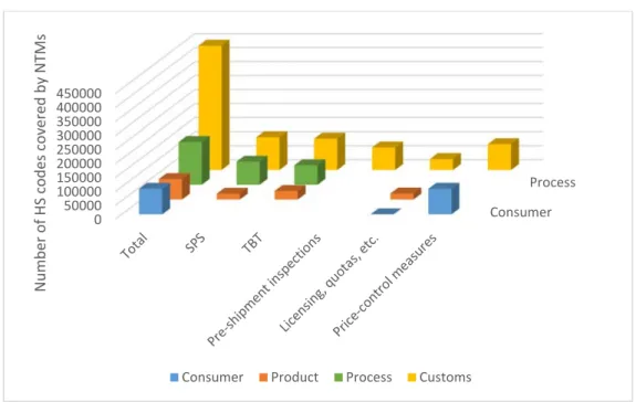
In an attempt to get a better handle on the effects of NTMs on trade, Ederington and Ruta (2016) introduced a functional categorization whose correspondence with the MAST classification at the HS6 line is shown in figure 3. MAST chapters represented in figure 2 are A Sanitary and Phytosanitary (SPS) measures, B Technical barrier to trade, C Pre-shipment inspection, E Non-automatic licensing, quotas, prohibitions and quantity- control measures other than for SPS or TBT reasons, and F Price-control measures, including additional taxes and charges. Chapters E to O were not considered due to data quality. Chapter P was not considered as it collects export measures. To their list, we add
18 The slightly higher average value for bilateral tariffs than for MFN is because some countries (notably China, Taiwan, Vietnam charge tariffs higher than MFN for some non-WTO members.
19 NTM data bases with large country and product coverage have several limitations, among which: (i) omissions and double counting; (ii) lack of precision (binary variables); (iii) time dimension (only new measures are notified); (iv) dimensionality (large number per HS6 line with strong multicollinearity across NTMs). Melo and Nicita (2018b) discuss these, and other, shortcomings in further detail.
20 See the discussion in Ing et al. (2016) who advocate that, because of their complexity, rather than try to negotiate-- yet again-- their removal, a process of regulatory control at the country level, especially in the context of RTAs where harmonization and MRA are easier to implement than at the plurilateral or multilateral levels.
NTMs classified as contingent trade-protection measures and local content measures.21 This gives
the estimated sample of NTMs and NTBs per product in our sample.
Figure 3: From Collecting agencies’ classifications to theory-based classification NTMs
Source: NTMs from MAST list according to authors’ classification (See text)
Figure 3 shows that the densest category is “Customs”, which refers to NTM applied at the border. Those NTM are also most likely to have a protectionist intent and be Non-Tariff Barriers (NTB) that hinder trade. Consumer, Process, and Products NTM categories may have an ambiguous effect on trade and are more likely to have a precautionary intent. Thus, we aggregate them together and consider them separately. This is a rough cut, but arguably, a plausible starting point at parsing out NTBs from the universe of NTMs.22
21 These are classified under categories D and I-01 in the MAST classification. Both types of measures were perceived as barriers to trade in a sample of 136 firms exporting EGs from 10 high-income countries. See Fliess and Kim (2008). 22 Ing et al. discuss how the three main categories of NTM costs (enforcement costs, sourcing costs and process-adaptation costs) affect simultaneously trade flows and market structure.
Consumer Process 0 50000 100000 150000 200000 250000 300000 350000 400000 450000 N u mb er of HS c od es c overed b y N TM s
Figure 4: Average number of NTMs and NTBs per product by list
Figure 4 shows the average number of NTMs and NTBs by income group across goods on each one of the three lists. These NTMs being collected as a binary variable on the presence (or absence) of a specific NTM does not allow one to appreciate their relative importance for restricting trade or for adding to trade costs. For example, differences in the number of NTMs applied across sectors or countries should not be unequivocally interpreted as regulatory stringency as one particular form of NTMs could be much more stringent than several NTMs combined. Moreover, equivalence in regulations does not necessarily imply equivalence in stringency as the implementation and enforcement of identical NTMs are different across countries, and therefore so are the effects. In sum, because of the very limited informational value from a count or NTMs (and a fortiori of NTBs), one should exercise caution in interpreting the estimates from the count of NTBs below.
Returning to figure 4, three patterns stand out. First is the confirmation of a larger average number of NTMs per HS product for the HIC group for the APEC and WTO lists. The NTM and NTB counts are much higher for the HIC group than for the other groups for those two lists, most probably a reflection that environmental objectives gain in importance as per capita income rises . Second, the patterns across groups are similar for the EPP list where the average number of counts on both NTMs and NTBs are quite similar across all income groups. This pattern is also consistent with the decision by negotiators to exclude NTBs from the negotiation agenda. Third, patterns are similar for NTMs and NTBs for the LIC and LMIC groups.
The NTMs and NTBs described in figure 4 are mostly non-discriminatory.23 Furthermore, about 82%
of the relationships exhibit no partner-level variation in the number of NTMs and NTBs applied. This is an issue for the gravity estimates reported in section 4 since the gravity framework is bilateral in nature where these non-discriminatory NTMs and NTBs are captured by the country-product fixed effects.
23 The standard deviation of the count of NTMs and NTBs applied within an importer – product relationship is about 0.03 on average, while the standard deviation in the between importer-product relationship is 12.2.
0 5 10 15 Si mpl e a ve ra ge numb e r of NTM /NT B p er pr oduct
High Upper middle Lower middle Low ApecEPPWTO ApecEPPWTO ApecEPPWTO ApecEPPWTO Average of number of NTM per product by income level
mean of nbr mean of ntb
Evidence shows however that harmonization of NTMs and NTBs matters for trade. It is recognized that a measure of regulatory overlap captures the often-found pattern of greater bilateral trade between countries that have greater regulatory overlap.24 To capture the extent of overlap, we take
the index developed by Knebel and Peters (2018). This index measures how closely two countries regulate their trade. Formally, the regulatory overlap is defined as follows:
∑ ∑
∑ ∑ (1)
In (1), is an index for importers; for exporters; for goods; NTM categories (as defined by the MAST classification). is a dummy equal to 1 when country imposes at least one NTM of type on good . The numerator is therefore the number of similar NTM applied by both countries and the denominator is the total number of NTMs applied by the importer. Hence the regulatory overlap is the share of NTMs applied by an importer which are also applied by the exporter. Note that, unlike with other measures of regulatory convergence or regulatory distance, this measure is not reflexive ( . For two countries and , a higher overlap will occur either if the number of similar NTMs between the two countries increases (i.e. there is regulatory harmonization between the two countries) or if the exporter eliminates the NTMs that he doesn’t share with the importer (i.e. there is deregulation).
The regulatory overlap is calculated for the “Process” and “Products” NTM categories, as defined by Ederington and Ruta (2016). These categories encompass NTMs which deal with how products are manufactured or with the characteristics of the products themselves. Dealing with those NTMs will require from the exporter side an adaptation of the production process or of the characteristics of the goods which will result in a single entry cost. Hence harmonization will favorize exporters as they will face similar requirements in their home and exporting markets, thus eliminating the costs associated with compliance. In contrast, the two other categories “Consumers” and “Customs” regroup NTMs addressing sales of goods and border management policies for which harmonisation is unlikely to affect trade flows. Indeed, costs induced by these NTM will be repeated for each sale or custom clearance. It is nonetheless important to note that while we concentrate on “Process” and “Products” NTM categories in our regulatory overlap measure, “Customs” and “Consumers” NTM are captured by fixed effects in the regressions reported in section 4.
24 Czubala et al. (2009) find that non-harmonization of African standards to those of the ISO strongly reduce African exports of textiles and Apparel and of other manufactures. Xiong and Beghin (2014) show that Maximum Residue Levels in plant products imposed by OECD countries jointly enhance import demand of OECD countries and hinders mostly export supplies of LDCs.
Figure 5: NTM overlap heatmap
The resulting regulatory overlap index theoretically goes from 0 (no NTM applied in common) to 1 (all NTMs are similar). In practice, the lowest observed overlap is 0 (for example between Togo and Kazakhstan) to 0.94 between El Salvador and the USA. Remember that the index is not reflexive: the value of the index between El Salvador and the USA is about 0.06 only, reflecting the fact that El Salvador relies on less process and products NTMs than the USA. The average overlap value in the dataset is about 0.21 with a standard deviation of 0.19.
Figure 5 presents the variation of the index between income groups. A darker shade represents a higher value for the index of regulatory overlap. The vertical axis represents the income group of the importer and the horizontal one those of the exporter. For example, an UMIC importing goods from a HIC exporter will face a high regulatory overlap on average (black shade with value of 0.37). Two patterns stand out from this heatmap. First, regulatory overlap measures increase with the level of the exporter’s income as one would expect since HICs tend to resort more to NTMs and thus are more likely to cover their counterparts’ NTM. Second the regulatory overlap of the LICs and MICs exporter tend to decrease with the income level of the importer. As importers are the reference for the regulatory overlap index this again reflects the fact that higher income countries apply more NTMs. Interestingly, high-income exporters exhibit the opposite pattern and their average regulatory overlap increases with the income level of the importers.
IV. Correlates of bilateral trade in EGs
A reduction in barriers to trade should increase trade volumes. Are there distinctive patterns for EGs vs. non-EGs, and how important are measures of the regulatory environment, as captured by the measure of regulatory overlap? Section 4.1 presents the methodology, section 4.2 reports elasticity estimates of trade to changes in tariffs and in regulatory overlap. Section 4.3 uses import demand elasticities to estimate the import response to a reduction in tariffs on EGs.
4.1 Structural Gravity model
LIC LMIC UMIC HIC Im po rt er 's in com e g rou p
LIC LMIC UMIC HIC
Exporter's income group
.117982 .164841 .211701 .25856 .30542 .352279 R e gu la tory ov er la p
To estimate the impact of reductions of tariffs and of regulatory harmonization on EG trade, we use the structural gravity trade model described in equations (2-4) where , are indices representing exporter and importer respectively and is an HS6 product level index that includes EGs and non-EGs. The model is:
(2)
Π ∑ (3)
P ∑ (4)
In equations (2-4), and are output and expenditures on good in the exporting (i) and importing (j) country respectively, is total endowment of good k across the sample of countries. Since this endowment is fixed for each good, changes in trade policy will be reflected in a reallocation of expenditures across partners for each product and a reduction in trade barriers on EGs will only lead to a reallocation of expenditures from non-EGs to EGs.25
Equation (2) says that bilateral trade flows are given by the product of a size term and a total trade cost term where is the expression for bilateral trade costs that included trade barriers (see (5) below). Equations (3 and 4) measure the repercussions of a change in bilateral trade costs between and to other partners through the terms Π , , defined as the outward (inward) multilateral resistance terms. These multilateral terms are aggregate of all bilateral trade costs. The outward multilateral resistance term in (3) is the weighted average of all bilateral trade costs for the producers of good in each country that measures market access for exporter of good when there is a change in trade policy (or other trade costs) between the two partners. Similarly, the multilateral trade cost term in (4) defines the inward multilateral bilateral trade cost as a weighted average of all bilateral trade costs that fall on consumers following this change in trade policy. Thus, these equations measure spillovers of changes in trade policy between two countries separately for other producers and consumers. In the estimation below, these multilateral resistance terms that are specific to each sector are captured by exporter-sector and importer-sector fixed effects. 26 An
important property of this class of gravity models is that the direct trade cost elasticity is constant 1 , where σ is the elasticity of substitution between products of different origin. This
25 This is why with endowments fixed, simulations of trade policy changes are ‘conditional’ (on output) general equilibrium effects However, output at the HS6 level are required to carry out conditional general equilibrium simulations. Because this data is not available simulations in section 4.3 are carried out for aggregate imports.
26 This presentation taken from Yotov et al. (2016, chp. 2 Appendix B) corresponds to the demand-side version of Anderson and Van Wincoop (2003). In other models from the supply side, another parameter takes the place of σ, here assumed to be the same across goods. What is important is that all these isomorphic formulations leading to the system (1)-(3) assume constant budget shares. This assumption has been questioned by Novy (2013) who shows that with a translog expenditure system instead of the CES system, the trade cost elasticity varies inversely with a country’s import share.
formulation precludes the possibility that trade is more sensitive to trade costs when the exporting country only provides a small share of the destination country’s imports.
The trade cost function is log-linear, expressed in terms of the following:
log log ∗ log _
log _ ∗ (5)
Taking the model to the data set described in section 3, we report estimates from equation 6 below.
exp log log ∗
log _ log _ ∗ ∗
(6)
In (6), is an index for exporters, is for importers, k is for product; log is the log of the applied bilateral tariff; log _ is the log of the measure of the regulatory overlap defined in (1); is a vector of bilateral controls comprising the log of distance between trading partners, dummies indicating if countries and share a common language, and a common border; and are importer-product and exporter-product dummies that control for omitted variables. The interactions should require the inclusion of an being equal to one when goods are on the considered EG list. This is not needed in our case as this dummy is already controlled for by the two country-product-level fixed effects.
With our focus on a disaggregated evaluation, the identifying assumption is that tariffs and NTBs are exogenous and that omitted variable bias is ‘adequately’ controlled by the country-product-level dummies for exporters and importers that capture the multilateral resistance terms and the vector of bilateral controls.
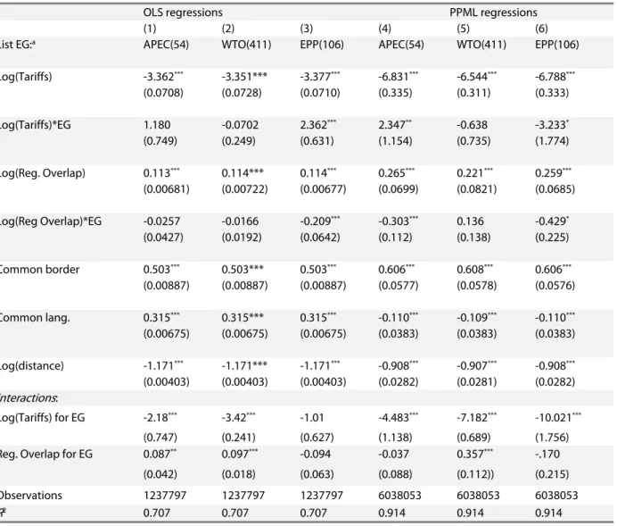
Because of the large number of zero trade flows (see the discussion of table 1 results) and heteroscedasticity, the model is estimated with the Pseudo Poisson Maximum Likelihood (PPML) estimator suggested by Santos Silva and Tenreyro (2006). As shown by a comparison of OLS estimates with PPML estimates in table 1, the large values for the OLS coefficient estimates are unrealistic. Another important advantage of the PPML estimator is that the multilateral resistance terms are directly recoverable from the PPML estimates (Arvis and Shepherd (2013)).
Our main interest is on the sign and coefficient values for the α and β coefficients that estimate the effects of barriers on bilateral trade and whether these barriers are significantly different across EG lists and between EG and non-EG lists. We expect negative and as a higher tax rate should diminish trade flows and a positive and as having a closer regulatory framework should increase trade flow as exporters do not incur extra costs to adapt their products to the destination’s requirements.
4.2 Trade Response to tariff reductions and to regulatory distance
As a preliminary check, table 1 compares results from OLS estimates (cols. 1 to 3) with those from PPML (cols. 4 to 6) for the APEC, WTO and EPP lists respectively. Three patterns stand out. First, about 80% of the possible country pair- product combinations are not traded… This accounts for the differences between coefficient estimates for the OLS in cols. 1 to 3 and the PPML in columns 4 to 6 and justifies reporting only PPML results in the following tables. Second, the bilateral controls have the expected sign and are highly significant. Third, as expected, reductions in barriers to trade and increases in regulatory overlap are positively correlated with bilateral trade flows.
Turn to the PPML results in cols. 4 to 6. Note first that for the WTO list with largest number of products (col. 5), that EGs do not exhibit any different behaviour than their non-EG counterpart (both interactions between EG and tariff and EG and regulatory overlap are not significant). This similarity reflects that, even though the list only represents about 8 percent of the total number of HS6 lines on the 1992 revision on the HS, any EG specificity of EGs is blurred. Consistently for all three lists, an increase in regulatory overlap increases bilateral trade in non EG tough EG on APEC and EPP lists are not affected by regulatory convergence. On average, a 10 percent increase in regulatory overlap increases bilateral trade in non-EG by approximately 2 percent. On average, the import tariff elasticity is -6 for the whole sample but elasticities are significantly different across the three EG lists. The average elasticity for the EG lists ranges from -10 for the EPP list with the highest tariff to -4 for the APEC list which has the lowest average tariff. These patterns are a reflection of the negotiators’ mercantilistic behaviour of excluding from the APEC (and to a lesser extent the WTO) lists EGs with high tariffs for which import demand would be most sensitive to tariff reductions.
Table 2 carries out estimates for the lower-income countries in the sample, those in (LIC+LMIC) group. In columns 1 and 2, estimates are restricted to the sample of developing (LIC +LMIC) importers in their bilateral trade with all countries. In columns 3 and 4, bilateral trade is for all importers, but exporters are restricted to developing (LIC+LMIC) countries. These two subsamples comprise 33% and 27% respectively of the total sample.27
27 Estimates for the APEC list are not reported because of the instability of estimates owing to the small number of goods in that list.
Table 2: Barriers to trade and HS6 level bilateral trade in EG: LIC and LMIC
LIC / LMIC importersa LIC / LMIC exportersb
(1) (2) (3) (4)
List EG: WTO EPP WTO EPP
Log(Tariffs) -4.983*** -6.260*** -7.846*** -7.956*** (0.463) (0.496) (0.743) (0.698) Log(Tariffs)*EG -4.440*** 5.149** -1.195 -0.530 (1.281) (2.562) (2.087) (3.543) Log(Reg. Overlap) 0.0517 0.0291 -0.0527 -0.0932 (0.0582) (0.0546) (0.0728) (0.0653) Log(Reg Overlap)*EG -0.0721 0.362** -0.230 -0.250 (0.137) (0.179) (0.148) (0.543) Common border 0.215*** 0.214*** 0.292** 0.296*** (0.0523) (0.0527) (0.114) (0.114) Common lang. 0.197*** 0.195*** 0.440*** 0.444*** (0.0731) (0.0736) (0.114) (0.114) Log(distance) -1.300*** -1.303*** -1.672*** -1.664*** (0.0421) (0.0431) (0.0736) (0.0735) Interactions: Log(Tariffs) for EG -9.422*** -1.110 -9.041*** -8.485** (1.228) (2.554) (1.983) (3.502)
Reg. Overlap for EG -0.204 0.391** -0.282** -0.343
(0.123) (0.169) (0.130) (0.538)
Observations 2001139 2001139 1674271 1674271
R2 0.959 0.959 0.971 0.971
Robust standard errors in parentheses * p < 0.10, ** p < 0.05, *** p < 0.01 Notes:
a Exporters from all country groupings b Importers from all country groupings
Several patterns appear when estimates are compared with those in table 1, cols. 4-6. First, the distance coefficient estimate is larger than in table 1, capturing the often-reported result of higher trade costs in bilateral trade when one of the partners is a lower income developing country.28
Second, the coefficient estimates on regulatory overlap are not statistically significant, a reflection of low regulatory barriers among these countries. Third, for both lists, import elasticities to tariffs are significantly different from non-EGs when the lower-income countries are importers (cols. 1 and 2) but not when they are exporters (cols 3 and 4). When developing countries are EG importer, the impact of tariff on EPP goods is not significant (Col. 2) while the impact of tariff for WTO’s EG exporter
28 Along the same lines, as a reflection of the low bilateral trade of the (LMIC +LIC) group with partners, the coefficient values for the common border dummy are lower than the corresponding ones in table 1.
(Col. 1)) is higher than its non-EG counterpart. When developing countries are EG exporters (Cols. 3 and 4), tariffs do not have a different impact on EG and non EG. Regulatory overlap yields no different impact for EG, with the exception of importers of EPP EG who face a greater benefit of regulatory overlap.
Estimates reported here are from lists drawn up through negotiations rather than from an attempt at definition of EGs from a set of agreed upon objectives. For example, one could carry out estimates for goods for environmental protection (e.g. equipment for monitoring pollution), for goods that are better that perform better than their substitutes (wind turbines or efficient refrigerators), for goods created in a green way (organic foods). In some instances, these goods feature already in the HS6 code, in others in others this would require creating new product codes.
4.3 Partial equilibrium estimates of changes in EG tariffs
With data on production at the HS6 level, the above estimates could be used to simulate the effects of changes in trade policy and regulatory policies as captured by the index of regulatory overlap. Not having expenditure at the HS6 level also precludes estimating welfare effects from tariff changes (e.g. Arkolakis et al. (2012)). Under these shortcomings, we exploit differences in tariff patterns by income group to give orders of magnitude of import response at the country level and aggregate them up to the income categories used in the descriptions of tariffs and NTBs in section 3.29 Since the pattern of tariffs in figure 1 differ markedly across income groups, with HS6 level import
demand elasticities, one can still simulate the effects of tariff changes at the country level and aggregate them by income category. Omitting country subscripts, the partial equilibrium formula for the change in imports following a unilateral change in tariffs for imports of an EG product is given by
Δ 1 ; Δ ≡ (7)
Where k is an index for EG goods; the exponents 0 and 1 represent the value of the variables before and after the policy change; is the value of imports of good ; Δ the change in imports due to the policy change; the applied bilateral MFN tariff before the policy change; is the magnitude of the policy change (if 1 then there is no change, 0.5 the tariff is halved, etc.); and is the import demand elasticity for good k, sourced from Kee, Nicita and Olarreaga (2008).
Table 3 reports the results for a 50% reduction in tariffs across-the-board for the two lists. Average import elasticities reported in Column 2 display falling values as one moves down from the HIC to the LIC group. This pattern confirms the claim that import demand elasticities are low for LICs, a reflection of the lack domestic substitutes. These patterns confirm the fears of the developing countries who have not participated in the submission of lists since a reduction in tariffs would not
29 The TiVA (trade in value-added data base) data set gives production data at the 3- digit ISIC level. However, low-income countries are largely under-represented in this data base making it unsuitable for a meaningful exercise in a paper that focusses on developing and, especially, low-income countries.
only result in larger government losses, but also probably in lesser welfare gains (at equal tariff rates).
Table 3: Simulated import response to a change in tariff by income group
Income group Initial trade volume1 Average import Elasticity2
Change in import volume1 Percentage change in Import volume
Tariff removed Tariff halved Tariff removed Tariff halved
(1) (2) (3) (4) (5)=(3)/(1) (6)=(4)/(1) APEC HIC 210186 -2.079 1549 741.3 0.737% 0.353% UMIC 124891 -1.910 5030 2276 4.03% 1.82% LMIC 15240 -1.866 1427 593.2 9.37% 3.89% LIC 714.9 -1.680 105.3 41.39 14.7% 5.79% EPP HIC 22354 -1.912 421.4 165.9 1.89% 0.742% UMIC 6637 -1.945 490.1 188.3 7.38% 2.84% LMIC 1799 -2.109 494.7 149.9 27.5% 8.33% LIC 157.3 -0.980 18.12 8.359 11.5% 5.31% Notes: 1 Million USD
2 Elasticity estimates at the country and HS6 levels from Kee, Nicita, and Olarreaga (2008). To reduce the weight of extreme observations, two modifications were made. For elasticities when calculating import responses, for each country in each income group, the estimates outside the 1st. and 9th decile were fixed at the respective decile cutoffs. We also eliminated 34 extreme estimates.
Columns 3 and 4 report estimated changes in import volumes by income group and columns 5 and 6 the corresponding percentage change in imports. Differences across group averages are the result of two effects working in opposing directions: high tariffs in the lower-income groups and lower elasticities for these groups. The patterns are dominated by differences in tariffs with very small changes for the HIC group and much greater ones for the LIC group.
V. Conclusions
Progress at reducing barriers to trade in Environmental Goods (EGs), viewed as essential in the move towards a green development path has, so far, been insignificant. High income countries (HICs) have failed to agree on lists, excluding goods in which they have tariff peaks and mostly selecting goods in which they have a revealed comparative advantage. Countries in other income group categories (UMICs, LMICs, and LICs) have not participated in the negotiations mandated at the start of the Doha Round. As documented in this paper, however, regardless of the selected list of EGs, their average applied bilateral tariffs are low at around 1 percent while average applied bilateral tariffs are higher across the other income groups. Because of concerns, with few exceptions—China and Costa Rica
— developing countries have not participated in the negotiations. Concerns include negotiation on lists that would include mainly industrial products and exclude Environmentally Preferable Products (EPPs) in which developing countries have a comparative advantage but which would meet resistance at the WTO. Fears also include little new access to markets where tariffs are already very low, an import surge in their own markets, and the fear that their domestic markets are too small to develop viable industries in EGs, if only because to develop EGs one needs environmental regulations in the first place.
To assess these fears, this paper assembled the largest possible sample of countries with data on tariffs and NTBs extracted from the most comprehensive list NTMs across countries for 2014, resulting in a sample of 51 countries with approximately the same number of countries across the four income groups. The paper also constructed a measure of regulatory overlap in bilateral trade to capture the often-observed pattern of greater bilateral trade among countries that share similar regulatory regimes.
In a first step, these measures of obstacles to trade were correlated with bilateral trade patterns across groups for two lists of EGs. One, the APEC list is representative of the interests of the HICs. The other, an EPP list, is indicative of the EGs that would have been selected by countries in the other income groups, had they participated in the negotiations. Patterns show that HICs negotiators, displayed mercantilistic behaviour by excluding from lists goods with high tariffs. Patterns also show that LICs have the lowest percentage of goods exported for all lists although their share of goods in which they have a revealed comparative advantage (RCA>1) is largest for the EPP list, and higher than the share for the HICs.
In a second step, estimates of a structural gravity model were reported. The broad conclusions of the exercise show that tariffs are still a significant barrier to bilateral trade, especially so for the EPP list but that generally import elasticities to applied bilateral tariff for EGs were not significantly different from those for non-EGs for the two lists. For all estimations, an increase in regulatory overlap that would result from regulatory harmonization would increase bilateral trade. Regulatory harmonization which would be carried out unilaterally or on a voluntary basis between partners would thus appear to be a promising avenue to move forward on the Doha mandate.
Finally, estimations for sub-samples only involving bilateral trade of LMIC and LIC partners with all other partners reveal higher trade costs (as captured by coefficient estimates of distance) for trade involving the lower-income countries in the sample. Subject to precautionary interpretation, calculations of import responses to tariff reductions across income groups suggest that the largest increases in imports of EGs would be for the lower-income groups. These results give support to some of the fears expressed by developing countries while, at the same time suggesting that, because of the higher tariffs for this group of countries welfare gains are likely to be largest for this group.
VI. Bibliography
Aichele, R., G. Felbermayr (2015) “Kyoto and Carbon Leakage: An Empirical Analysis of the Carbon Content of Trade”, Review of Economics and Statistics, vol. 97, pp.104-11.
Antweiler, W., B. Copeland, M. Taylor (2001) “Is Free Trade Good for the Environment?” The American Economic Review, vol. 91, pp. 877-908.
Arkolakis, C., A. Costinot, A. Rodriguez-Clare (2012) “New Trade Models, Same old Gains”, American Economic Review.
Arvis, J.F., Shepherd, B.A. (2012) "The poisson quasi-maximum likelihood estimator: a solution to the "adding up" problem in gravity models (English)", Applied Economics Letters, vol. 20 (6), pp. 1-11.
Bacchus, J. (2018) “Triggering the Trade Transition: The G20’s Role in Reconciling Rules for Trade and Climate Change”, Geneva: International Centre for Trade and Sustainable Development (ICTSD).
Baier, S.L., Bergstrand, J.H. (2007) "Do free trade agreements actually increase members' international trade?", Journal of International Economics, vol. 71(1), pp. 72-95.
Balineau, G., J. de Melo (2013) “Removing Barriers to Trade on Environmental Goods: An Appraisal”, World Trade Review, vol. 12, pp. 693-718.
Baghdadi L., Martinez-Zarzoso I., Zitouna H. (2013) “Are RTA agreements with environmental provisions reducing emissions?”, Journal of International Economics, vol. 90, pp. 378–390.
Barrett, S., C. Carraro, J. de Melo (2015) “Towards a Workable and Effective Climate Regime”, CEPR, 548 p.
Bucher, H., J. Drake-Brockman, A. Kasterine, M. Sugathan (2014) “Trade in Environmental Goods and Services: Opportunities and Challenges”, ITC, Geneva.
Cherniwchan, j., B. Copeland, M.S. Taylor (2017) “Trade and the environment: new methods, measurement and results”, Annual Review of Economics, vol. 9, pp. 59-85.
Cosbey, A. (2014) “The Green Goods Agreement: Neither Green nor Good?”, IISD.
Czubala, W., B. Shepherd, J. Wilson (2009) “Help or Hindrance: The Impact of Harmonizing Standards on African Exports”, Journal of African Economies, vol. 18 (5), pp. 711-44.
Ederington J., M. Ruta (2016) “Non-tariff measures and the world trading system”, Handbook of Commercial Policy, Elsevier, North-Holland, also World Bank PRWP #7661.
Esty, D.C. (1994) “Greening the GATT: Trade, Environment, and the Future”, Institute for International Economics, Washington D.C, 319 p.
Fliess, B., J. Kim (2008) “Non-Tariff Barriers Facing Trade in Environmental Goods and Associated Services”, Journal of World Trade, vol. 42 (3), pp. 535-62.
Fischer, C. (2010) “Does Trade Help or Hinder the Conservation of Natural Resources”, Review of Environmental Economics and Policy, vol. 4 (1), pp. 103–121.
DOI: https://doi.org/10.1093/reep/rep023
Grether, J.M., N. Mathys, J. de Melo (2012) “Unravelling the World-Wide Pollution Haven Effect”, Journal of International Trade and Development, vol. 21(1), pp. 131-62.
Hanson, G., C. Xiang (2004) “The Home-Market Effect and Bilateral Trade Patterns”, The American Economic Review’, vol. 94(4), pp. 1108-29.
Hummels, D., V. Lugovsky (2009) “International Pricing in a Generalized Model of Ideal Variety”, Journal of Money, Credit and Banking, vol. 41, pp. 3-33.
Ing, L, O. Cadot, S. Urata, R. Anandhika (2016) “Non-Tariff Measures in ASEAN: A Simple Proposal”, FERDI Working Paper No. 183.
Kee, H.L., A. Nicita, M. Olarreaga (2008) “Import Demand Elasticities and Trade Distortions”,