Building the big picture : enhanced resolution from coding

(1)

Building the BIG Picture:

Enhanced Resolution from Coding

by

Roger George Kermode

B.E. (hons) Electrical Engineering, University of Melbourne, 1989

B.Sc. Computer Science, University of Melbourne, 1990

Submitted to the Program in Media Arts and Sciences, School of Architecture and Planning,

in Partial Fulfillment of the requirements of the degree of MASTER OF SCIENCE IN MEDIA ARTS & SCIENCES

at the

Massachusetts Institute of Technology June 1994

Signature of Author

Program in Media Arts and Sciences

A May 6, 1994

Certified by

A few B. Lippman Asocire Director, MIT Media Lboratory Thesis pervisor Accepted By

-V

_{Stephen A. Benton}

Chairperson Departmental Committee on Graduate Students Program in Media Arts and Sciences

Rftch

MASSACHUSFETTS INSTITUTE

(2)

Building the BIG Picture:

Enhanced Resolution from Coding

by

Submitted to the Program in Media Arts and Sciences, School of Architecture and Planning,

on May 6, 1994

in Partial Fulfillment of the requirements of the degree of

MASTER OF SCIENCE IN MEDIA ARTS & SCIENCES

Abstract

Video Coding Algorithms based on Hybrid Transform techniques are rapidly reaching a limit in compression efficiency. A significant improvement requires some sort of new rep-resentation -- a better model of the image based more closely on how we perceive it. This thesis proposes a coder that merges psycho-visual phenomena such as occlusion and long-term memory with the architecture and arithmetic processing used in a high quality hybrid coder (MPEG). The syntactic and processing overhead at the decoder is small when com-pared to a standard MPEG decoder.

The final encoded representation consists of a small number of regions, their motion, and an error signal that corrects errors introduced when these regions are composited together. These regions can be further processed in the receiver to construct a synthetic background image that has the foreground regions removed and replaced, where possible, with revealed information from other frames. Finally, the receiver can also enhance the appar-ent resolution of the background via resolution out of time techniques. It is anticipated that this shift of intelligence from the encoder to the receiver will provide a means to browse, filter, and view footage in a much more efficient and intuitive manner than possible with current technology.

Thesis Supervisor: Andrew B. Lippman

Title: Associate Director, MIT Media Laboratory

This work was supported by contracts from the Movies of the Future and Television of Tomorrow consortia, and ARPA/ISTO # DAAD-05-90-C-0333.

(3)

Building the BIG Picture:

Enhanced Resolution from Coding

by

The following people served as readers for this thesis:

Reader:

Edward H. Adelson Associate Professor of Vision Science Program in Media Arts and Sciences

Reader:

Michaeff3 iggar Principal Engineer, Customer Services and Systems Telecom Australia Research Laboratories, Telstra Corporation Ltd.

(4)

To myfamily; George, Fairlie, Ivy May, and Meredith, whose love, support, and understanding made this thesis possible.

(5)

List Of Figures

Fig. 1.1 Genus of the Enhanced Resolution Codec ... 14

Fig. 2.1 Basis Functions for an 8 by 8 Two Dimensional DCT ... 21

Fig. 2.2 Huffman Coding Example ... 25

Fig. 2.3 Progressive and Interlace Scanning ... 27

Fig. 2.4 Block Based Motion Compensation Example ... 29

Fig. 2.5 MPEG2 Encoder Block Diagram...32

Fig. 2.6 MPEG2 Decoder Block Diagram ... 33

Fig. 3.1 Salient Still Block Diagram [28] ... 34

Fig. 4.1 An arbitrary one dimensional sequence, ... 40

Fig. 4.2 Sub nyquist sampled sequences, from odd and even Samples of Figure 4.1 ... 41

Fig. 4.3 Spectral Analysis of Down Sampling ... 42

Fig. 4.4 Four Camera Rig for Doubling Spatial Resolution...43

Fig. 4.5 Desired Camera response for doubling resolution...43

Fig. 4.6 Camera CCD Array (modified from Fig 2.22 in [5])...44

Fig. 4.7 Low pass frequency response due to finite sensor element size...45

Fig. 4.8 Two dimensional pulse train ... 46

Fig. 4.9 Modulation Transfer Function for a typical ccd array ... 46

Fig. 4.10 Modulation Transfer Function for a typical camera ... 48

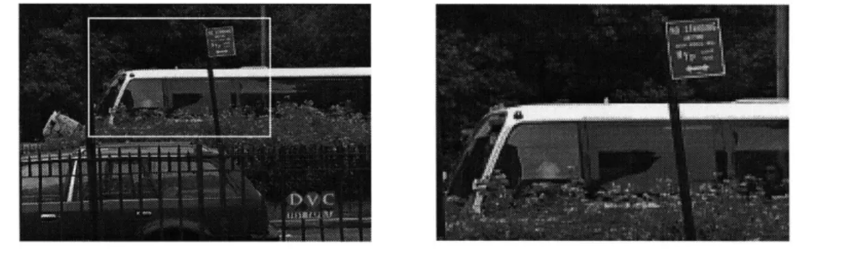
Fig. 4.11 Two Shots of the Same Scene a) Wide angle, b) Close up (2 X) ... 50

Fig. 4.12 Spectral Content of two pictures when combined ... 51

(9)

Fig. 5.1 Flower Garden Scene (from an MPEG test sequence) ... 57

Fig. 5.2 Variance Based Adjustment... 62

Fig. 5.3 Example of region allocation by scan line conversion and merge...63

Fig. 5.4 Example Region pruning ... 64

Fig. 6.1 Example of MPEG frame ordering ... 66

Fig. 6.2 Enhanced Resolution Codec Frame Ordering Example ... 69

Fig. 6.3 Enhanced Resolution Encoder Block Diagram...73

Fig. 6.4 Enhanced Resolution Decoder Block Diagram ... 74

Fig. 7.1 Original image and Segmented Lecturer with hole in head (and also in arm ) ... 76

Fig. 7.2 Poor segmentation due to flat regions causing inaccurate motion estimation...77

Fig. 7.3 Carousel Foreground Segmentation...77

Fig. 7.4 Super Resolution Backgrounds for frames 1, 51, and 89...79

Fig. 7.5 Super Resolution Frame with foreground composited on top ... 80

Fig. 7.6 Motion Information bit rates for the Lecturer Sequence...81

Fig. 7.7 Motion Information bit rates for the Carousel Sequence...82

Fig. 7.8 SNR for the Lecturer Sequence ... 83

Fig. 7.9 SNR for the Carousel Sequence... 84

Fig. A. 1 Pyramid Decomposition ... 88

Fig. A .2 Spiral Search M ethod... 91

(10)

Chapter 1 Introduction

1.1 Motivation

Hybrid transform video compression coders have been the subject of a great deal of

research in the past ten years, and within the last three, they have become practical and

cost effective for applications ranging from videotelephony to entertainment television.

They are the object of optimization rather than basic research. In fact, the sheer size of their expected deployment will effectively freeze their design until general purpose

pro-cessors can perform fully programmable decoding. The current state of the art provides

compression ratios on the order of 50 to 100:1 with acceptable loss of picture quality for

home entertainment.

Drawing a parallel with word processing, one could say that the level of sophistication

of these coders is currently on a par with word processors of 15 years ago. These early

word processors stored text very efficiently using codes of 7 to 8 bits per character, but

unfortunately the final representations included little information about the text itself. No

information concerning typefaces, page layout, or other higher levels of abstraction was

included in the representation. Today the majority of word processors allow one to format

text with a veritable plethora of options ranging from the size and style of font to

auto-matic cross referencing between text in different documents. It is easy to see that

embel-lishing the presentation with information about the text has made today's word processors

(11)

When one examines encoded video representations today one finds that they are at the 'text only' stage. Current algorithms do a very good job at reducing the size of representa-tion, but in doing so lose almost all ability to manipulate the content in a meaningful fash-ion. The much heralded information super highway with multi-gigabit data paths is expected to become a reality soon. When it does, it will be crucial that new representations be found for video that enable one to make quick decisions about what to watch without having to search through every single bit.

These representations should contain information about the content that enable

machine and viewer alike to make quick decisions without having to examine every

sec-ond of video. Without these representations the benefits of having access to an information

super highway, as opposed to access to traditional media sources will be minimal for all

but the expert user. This being the case, it will be difficult to attract people to use the

high-ways and it may become difficult to justify their cost.

Admittedly these are very lofty goals, the amount of effort required to achieve them is

enormous. Given the amount of effort required, and the newness of the super highway as a

medium, it is likely that the realization of these goals will take quite some time.

Conse-quently, if for no other reason than cost, it is also likely that the initial steps towards

(12)

1.2 The problem

Before a new representation can be derived it is useful to examine current state of the art

video coding algorithms in order to determine what their good and bad points are. The

salient features of current hybrid transform algorithms can be summarized as follows;

. Heavy reliance on statistical models of pictures, in particular

spatiotem-poral proximity between frames.

. The model used for predicting subsequent frames consists of only one or

two single frames that have previously been encoded.

. Frames are subdivided into blocks which are then sequentially encoded

using a single motion vector for each block and an error residual.

. Image formation by 3D to 2D projection is ignored; little consideration

is given to phenomena such as occlusion, reflection, or perspective.

. There is no easy means for determining the contents of a frame without

decoding it in its entirety.

Current research into new approaches to coding generally attempt to address different

sets of applications, or use radically different image models. For example, the MPEG'

group, which has issued one standard for multimedia and broadcast television (MPEG-1)

and is putting the final touches on another (MPEG-2 [3]), is beginning a three-year effort

deliberately designed to speed the evolution of radically different coders that break the

hybrid/DCT mold. These are expected to be used primarily in extremely low-bandwidth

applications, but the development spurred by the MPEG effort may extend itself past that.

(13)

As may be surmised from the list of hybrid transform coder features on the previous

page, these new modelling techniques derive from either new work on understanding

human vision (and mapping that into a compression system), or work on new

computa-tional efficiencies that permit complex models to be exploited that previously had been

academic tours de force.

1.3 Approach

This thesis proposes an object-oriented coding model that is an architectural extension to

existing MPEG-style coders. The objective model assumes no knowledge other than data

contained in the frames themselves (no hand-seeded model of the scene is used), and is

basically two or two-and-a-half dimensional (two dimensional plus depth of each two

dimensional layer). The model classifies objects within the frame on the basis of their

appearance, connectivity, and motion relative to their surrounds. While the raster-oriented

decomposition of the frame (as used in MPEG) remains in this coder, the image is no

longer coded as blocks classified on an individual basis. Instead, the image is coded as a

montage of semi-homogenous regions in conjunction with an error signal for where the

model fails.

The structure of the coder borrows many elements from previous coders and image

processing techniques in particular MPEG 2 [3], Teodosio's Salient Still [28] and the work

by Wang, Adelson and Desai [4], [30]. The resulting coding model incorporates the

effi-ciencies of motion compensation using 6 parameter affine models as well as the increased

accuracy of standard block based motion compensation for foreground regions that do not

match the affine model. It is hoped that the coding scheme developed here may eventually

(14)

by Holtzman [13] which promises extremely high compression ratios. The genealogy of the Enhanced Resolution Coder is shown in Figure 1.1.

H.261, MPEG1, H.262 (MPEG2)

Salient Still (Teodosio) 'nhancpd Rp.vnlutinn Cnrlpr Image Encoding &

Representation Schemes

Layered Coder, (Adelson & Wang)

Full 3D Coder (Holtzman)

>Full

3D Coder (automatic)

Genus of the Enhanced Resolution Codec

Another way to classify the algorithm is to consider its position in the table below,

Encoder Type Information Units Example

Waveform Color D1

Transform Blocks JPEG [1]

Hybrid Transform Motion+ Blocks MPEG [3], [12] 2D Region Based Regions + Motion + Blocks Mussman's Work [21]

Layered Coder [4], [30] Enhanced Resolution Coder Scenic 3D Objects "Holtzman Encoder" [13] Semantic Dialogue, Expressions Screenplay

Encoder Classes (after Mussman)

Another motivating advantage of such a structural analysis of the image is that the

structure can be exploited at the receiver, without any additional recognition, to facilitate

browsing, sorting sequences, and selecting items of interest to the viewer. In essence, the

pictures are transmitted as objects that are composited to form a frame on decoding, and

Figure 1.1.

(15)

each picture carries information about the scene background, the remaining foreground

objects, and the relation between them. As compressed video becomes pervasive for

enter-tainment, it is anticipated that "browsability" of the sequence will become at least as

important as the compression efficiency to the viewer, for there is little value in having

huge libraries of content without a means to quickly search through them to find entries of

interest.

With these ideas in mind, the target application of the televised lecture was chosen to

demonstrate the enhanced resolution codec. The reasons behind this decision are

three-fold. First, the scene is best photographed with a long lens that minimizes camera

distor-tion (this is a requirement for optimal performance). Secondly, enhancing the resoludistor-tion of

written or projected materials in the image will allow the viewer to see the material at a

finer resolution, while still seeing a broader view of the lecture theatre. In fact the

algo-rithm will allow the viewer to determine whether the entire scene or just the

written/pro-jected material is displayed. This feature is particularly useful as it allows the user to

choose the picture content according to interest and decoder ability (small vs large screen).

Finally, apart from technical considerations the aforementioned application has the

poten-tial to provide a useful service to students who, for whatever reason, have insufficient

teaching facilities available, thus allowing them to participate in lectures from other

schools and institutions

The remainder of this thesis is organized as follows. Chapter Two briefly reviews the

fundamentals of encoding still and moving images. Chapter Three examines three recent

advances in image representation. An analysis of the theory behind resolution

enhance-1. One such program of televised lectures is already been undertaken by Stanford University which regularly broadcasts lectures via cable to surrounding institutions and companies who have employees enrolled in Stanford' classes. Livenet in London, England and Uninet in Sydney, Australia are also other examples of this type of program.

(16)

ment is presented in Chapter Four. Chapters Five and Six map the results of the previous

chapters into a frame work that defines the new encoder. Simulation results of the new

algorithm, including a comparison with the MPEG1 algorithm, are presented in Chapter

Seven. Finally, Chapter Eight presents an analysis on the performance of the new

algo-rithm and makes suggestions for future work.

Necessary and self contained technical derivations of various mathematical formulae

(17)

Chapter 2 Image Coding Fundamentals

Currently all displayed pictures, whether static or moving, are comprised of still

(station-ary) images. For example, photographs, television images and movies are sequences of

one or more still images. This representation has not come about by accident but instead

by design. As one Media Lab professor is fond of saying "God did not invent scanlines

and pixels... .people did". Therefore, it is not surprising that the current image coding

tech-niques for moving tend to be based on philosophies very similar to those used for

encod-ing still images, mainly that of spatio temporal redundancy and probabilistic statistical

modeling. This chapter examines these philosophies as they have been applied in

develop-ment of the JPEG' and MPEG standards for still and moving image coding respectively.

2.1 Representation

The choice of representation affects two fundamental characteristics of the coded image;

. Picture Quality

. Redundancy present in the representation

These two characteristics are independent up to a point, generally one can remove

redundant information from a representation and not suffer any loss in picture quality, this

is lossless compression. However, once one starts to remove information beyond that

which is redundant the picture quality degrades. This type of compression, where non

redundant information is deliberately removed from the representation, is known as lossy

(18)

compression. The amount and nature of the degradation caused by the use of lossy

com-pression techniques is highly dependent on the representation chosen. Hence, it makes

sense that great care should be exercised in choosing an appropriate representation when

using lossy compression techniques.

2.2 JPEG Standard [1]

The Joint Photographic Experts Group (JPEG) standard for still image compression is

fairly simple in its design. It is comprised of three main functional units; a transformer, a

quantizer, and an entropy coder. The first and last of these functional units represent

loss-less processes1 with the second block, quantization, being responsible for removing

per-ceptually irrelevant information from the final representation. Obviously, if one desires

high compression ratios then more information has to be discarded and the final

represen-tation becomes noticeably degraded when compared with the original.

2.2.1 Transform Coding

A salient feature of most images is that they exhibit a high spatial correlation between the

pixel values. This means that representations in the spatial domain are usually highly

redundant and, therefore, require more bits than necessary when encoded. One method

which attempts to decorrelate the data to facilitate better compression during quantization

is Transform Coding. Transform Coding works by transforming the image from the spatial

domain into an equivalent representation in another domain (e.g. the frequency domain).

The transform used must provide a unique and equivalent representation from which one

can reconstruct all possible original images. Consider the general case where a single one

dimensional vector x = [x ,..., xk] is mapped to another u = [u ,..., Uk] by the trans-form T,

(19)

u = Tx (1.1)

The rows of the transform T, ti are orthonormal, that is they satisfy the constraint

7 0, ifi#j tit. ={ I j I1, ifi

=j

or _{TT = I} i.e. 7 1 ₌ (1.2)

The vectors t1, ..., t, are commonly called the basis functions of the transform T. The fact that they form an orthonormal set is important as it ensures that;

. they span the vector space of x in a unique manner, and

- the total energy in the transform u is equal to that of the original data x.

In other words, this property ensures that there is a unique mapping between a given

trans-form u and the original data x'.

Transforming from the spatial domain into another domain gains nothing in terms of

the number of bits required to represent the information. In fact, the number of bits

required to represent the transformed information can increase. The gain comes in that the

transformed representation can be quantized more efficiently. This is due to the fact that

the transform coefficients have been decorrelated and have also undergone energy

com-paction, thus many of them can be quantized very coarsely to zero.

1. The mathematics above deal with data that is represented by one dimensional vectors, however pictures are two dimensional entities. This is not a problem as one can simply extend the concept of transformation into two dimensions by applying a pair of one dimensional transforms performed horizontally and vertically (or vice versa).

(20)

JPEG uses the Discrete Cosine Transform (DCT) to reduce the amount of redundancy

present in the spatial domain. The image to be coded is subdivided into small blocks(8 by

8 pixel) which are then individually transformed into the frequency domain. Unlike the

Discrete Fourier Transform (DFT) which generates both real and imaginary terms for each

transformed coefficient, the DCT generates real terms when supplied with real terms only.

Thus, the transform of an 8 by 8 pel block yields an 8 by 8 coefficient block, there is no

expansion in the number of terms. However, these terms require more bits, typically 12

bits to prevent round off error as opposed to 8 in the spatial domain, so the representation

is in fact slightly larger.

The formulae for the N by N two dimensional DCT and Inverse DCT (IDCT) are

DCT 2 N-IN-I _{(2x + 1) ui} _{(2y + 1) vn}

F(u,v) =N _{C (u) C (v) 1}

_f(x,y)cos

₍ _N

₎

_{cos (}

N

IDCT 2 N- 1N-I (2x+1)tnC (2y+1)vn

f(x,y) = N 1 , C (u) C (v) F(u,v)cos N ) cos ( N

u=Ov=0

with u,v,x,y = 0, 1,2, ... N-1

where x, y are coordinates in the pixel domain u, v are coordinates in the transform domain

1

C(u), C(v) =

{F

for u, v =0

1 otherwise _(1.3)

The means by which a gain in compression efficiency can be achieved (by subsequent

quantization) lies in the distribution of the transformed coefficients. A corollary of the fact

that real world images exhibit high spatial correlation, is that the spectral content of real

world images is skewed such that most of the energy is contained in the lower frequencies.

Thus, the DCT representation will tend to be sparsely populated and have most of the

(21)

intuitively obvious when one examines the basis functions for the DCT as shown in Figure

2.1.

Increasing Horizontal Frequency

up

dct-basis(x,y) 1 2 3

m u.

mu,

Eu.

4

5

6

7 MEM.

MEE

NEu

Figure 2.1 Basis Functions for an 8 by 8 Two Dimensional DCT

The basis functions depicted towards the upper left corner correspond to lower

frequen-cies while those towards the lower right correspond to higher frequenfrequen-cies. The magnitude

of the transform coefficient corresponding to each of the basis functions describes the

'weight' or presence of each basis function in the original image block.

r) CD CD -t CD CD C

0 ofl

1

2

3 -6

(22)

7-2.2.2 Quantization of Transform Coefficients

Having transformed the image into the frequency domain JPEG next performs

quantiza-tion on the coefficients of each transformed block.

The coefficients corresponding to the lower frequency samples play a larger role in

reconstructing the image than the coefficients corresponding to higher frequencies. This is

true not only by virtue of the fact that they are much more likely to be present as stated in

Eq. 2.2.1, but also because perceptually the human visual system is much more attuned to

noticing the average overall change in image intensity between blocks as opposed to the

localized high frequency content contained in the higher frequency coefficients1. Thus, a

given distortion introduced into a component that represents low frequencies will be much

more noticeable than if the same distortion was introduced into a component that

repre-sents high spatial frequencies.

The DC (zero frequency) coefficient is particularly susceptible to distortion errors, as

an error in this coefficient affects the overall brightness of the block. For this reason the

DC coefficient is quantized with a much finer quantizer than that used for the remaining AC (non zero frequency) coefficients. Likewise, lower frequency AC components are

quantized less aggressively than higher frequency ones.

2.2.3 Entropy Coding

The final stage of the JPEG compression algorithm consists of an entropy coder. Entropy

is generally defined to be a measure of (dis)order or the amount of redundancy present in a

collection of data. A set of data is said to have high entropy if its members are independent

1. (Having said this it must be noted that if an image composed of inverse transformed blocks is displayed where the high frequency coefficients have been removed from all but a few of these blocks then those few blocks will be highly noticeable. For this reason it is desirable to attempt to discard the same number of higher coefficients in each block.)

(23)

or uncorrelated. Conversely, a set that displays high dependency or correlation between its

members is said to have low entropy. Given a set of symbols and their relative

probabili-ties of occurrence within a message, one can make use of this concept in order to remove

redundancy in their encoded representation.

First, consider a set of data which is completely random, in other words one where

every symbol is as likely as another to be present in a coded bitstream. Suppose that a

restriction is imposed which states that each symbols' encoded representation is the same

length. As each symbol is the same length in bits and just as likely to occur as another they

all cost the same to transmit, the representation is efficient. Now consider the case where

the symbol probabilities are not equal. It is easy to see that even though certain symbols

hardly ever occur they will still require just as many bits as the more frequent ones,

there-fore, the representation is said to be inefficient.

Now suppose that the restriction that all symbols be represented by codes of the same

length is relaxed, thereby allowing codes of different lengths to be assigned to different

symbols. If the shorter codes are assigned to more frequently used symbols and the longer

codes to the less frequent, then it should be possible to reduce the number of bits required

to encode a message consisting of these symbols. However several problems arise out of

the fact that the codes are of variable length;

. the position of a code in the encoded bit stream may no longer be known

in advance,

. a long code may by missed if it is mistaken for a short code.

As a result, great care must be taken to ensure that no ambiguities arise when assigning the

(24)

knowing where the previous code finished as this automatically provides the starting

posi-tion for its successor.

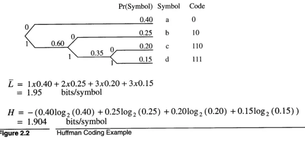
JPEG uses the results from a Huffman coding scheme based on this concept. It is

use-ful to introduce two equations ([15],[19]23]); first the average code word length L for

the discrete random variable x describing a finite set of symbols is defined as

L = XL (x) p, (x) bits/symbol (1.4)

x

and secondly, the entropy of x, H (x) , defined by Eq. (1.5), is the lower bound on L

H (x) = -jpx (x) log 2 (x) bits/symbol (1.5)

x

In short, the aim of entropy coding is try to make L as close as possible to H (x) . If

L = H (x) then all the redundancy present in x will have been removed and hence any attempt to achieve even greater compression will result in loss of information. This is a

theoretical limit and is seldom reached in practice. However it should be noted that higher

compression ratios may be achieved without loss by choosing a different representation

for the same information. The theoretical limit has not been violated in these cases. What

happens is that the pdf of x changes, resulting in a change of H (x) which falls below

H (x) of the original representation. Thus it makes sense to choose the most efficient rep-resentation before quantizing and subsequent entropy coding.

Huffman coding makes several big assumptions; first, that the probability distribution of

the set of symbols to be encoded is known and secondly that the probabilities do not

change. Given that these assumptions hold, the codebook containing the code for each

(25)

decoder or transmitted once by the encoder to the decoder at the beginning of a

transmis-sion.

The algorithm used to design these codebooks is very simple and constructs a binary

tree that has the symbols for leaves and whose forks describe the code. The probability of

each symbol is generated by performing preliminary encoding runs and recording the

fre-quency of each symbol in the final representation. Provided sufficiently representative

data is used to generate these symbols, the actual probability of occurrence of each symbol

may be approximated by its relative probability in the preliminary representation.

For a set of n symbols the algorithm constructs the tree in n - 1 steps where each step involves creating a new fork that combines the two nodes of highest probability. The new

parent node created by the fork is then assigned a probability equal to the sum of the

prob-ability of its two children. A simple example is shown below in Figure 2.2

Pr(Symbol) Symbol Code 0.40 a 0 60 0.25 b 10 1 0.60 0.20 c 110 1 0.35 1 0.15 d 111 L = 1x.40+2x0.25+3x0.20+3x0.15 = 1.95 bits/symbol H = - (0.4010g2 (0.40) + 0.2510g2 (0.25) + 0.2010g2 (0.20) + 0.151og2(0.15)) = 1.904 bits/symbol

Figure 2.2 Huffman Coding Example

Several codebooks generated by a method similar to that described above are used

(26)

2.3 Frame Rate

When one moves from still images to moving images comprised of a series of still images,

one of the main things that must be taken into account is the rate at which pictures are

pre-sented to the viewer. If too few pictures are prepre-sented to the viewer then any motion within

the picture will appear jerky, the viewer will notice that the moving image is not

continu-ous but in fact comprised of many separate still images. However, if the frame rate is

increased to a sufficiently high rate then the still images will "fuse" causing motion within

the picture to appear smooth and continuous.

The frame rate at which fusion occurs is known as the critical flicker frequency (cff)

and is dependent upon the picture size, ambient lighting conditions, and the amount of

motion within the frame [17] & [23]. For example when a T.V. screen is viewed in a

poorly lit room the cfff decreases, conversely the cfff increases when the same T.V. screen

is viewed in well lit conditions. The cfff also increases with picture size, which explains

why motion pictures are shot at 24 frames per second and then projected at 72 frames per

second with each frame being shown three times.

Standard television uses a special method to increase the temporal resolution without

increasing the bandwidth of the transmitted signal or decreasing the spatial resolution by

an inordinate amount. This trick is known as interlace and involves transmitting the

pic-ture as two separate fields; the even lines of the picpic-ture are sent in the first field, followed

by the odd lines in the second field. Transmitting a picture in this manner means that the

perceivable spatial resolution of the displayed image is larger than one field alone but

smaller than if both fields had been transmitted simultaneously (progressive scanning).

The gain comes in that the temporal resolution is increased beyond that of a system where

(27)

made to allow for better temporal resolution without increasing the number of scanlines

per unit time.

Progressive Scanning Interlaced Scanning

frame n - 2 frame n - 1 frame n fO fl fO fl fO fi frame n - 2 frame n - 1 frame n

fO = field 0, even scan lines fI = field 1, odd scan lines Figure 2.3 Progressive and Interlace Scanning

While interlace is appropriate and useful for analog televisions that only display

picto-rial information, it is particularly bad for computer generated text or graphics. When a

normal television displays these sorts of artificial images the human eye fails to merge the

spatial information in successive fields smoothly, and the 30 (NTSC)/ 25(PAL) Hz flicker

becomes painfully obvious. For this reason, there has been a concerted push towards

higher frame rates both for large screen computer monitors and emerging HDTV system

proposals. These HDTV systems will need these higher frame rates to support a larger

pic-tures. In addition, higher frame rate will also be needed to support the anticipated

com-puter driven applications made possible by the digital technology used to deliver and

decompress the images they will display. Some common frame rates used within the

movie, television and computer industries are 24, 25, 29.97, 30, 59.94, 60 and 72 frames

(28)

2.4 MPEG Standards [2], [3]

The Moving Picture Experts Group (MPEG) standard MPEG 1 [2] and draft standard

MPEG2 [3] are based on the same ideas that were used in the creation of the JPEG

algo-rithm for still images. In fact, MPEG coders contain the same transform, quantization and

entropy coding functional blocks as the JPEG coder. The difference between the MPEG

and JPEG coders lies in the fact that the MPEG coders exploit interframe redundancy in

addition to spatial redundancy, through the use of motion compensation. The three

stan-dards can be differentiated as follows;

. JPEG compresses single images independently of one another.

. MPEG 1 is optimized to encode picture at CD-ROM rates of around 1.1

Mbit/s at resolution roughly a quarter of that for broadcast TV by predicting

the current picture from previously received ones.

. MPEG2 inherits the features present in MPEG 1 but also includes

addi-tional features to support interlace and was optimized for bit rates of 4

and 9 Mbit/s

2.4.1 Motion Estimation and Compensation

Many methods for estimating the motion between the contents of two pictures have been

developed over the years. As motion estimation is only performed in the encoder and

hence the method chosen does not impact on interoperability, MPEG does not specify any

particular algorithm for generating the motion estimates. However, in an effort to limit

decoder complexity and increase representation efficiency, the decision was made that

motion vectors should be taken to represent constant (i.e. purely translational) motion for

(29)

grouping of a small number of blocks used by the DCT stage, thus allowing the decoder to

decode each tile in turn with a minimal amount of memory. Consequently, the most

com-mon method used to generate motion information for MPEG implementations is the block

based motion estimator.

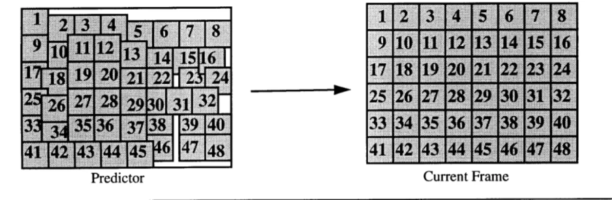
Block based motion estimators are characterized by the fact that they generate a single

motion vector to represent the motion of small (usually square) group of pels. The motion

vector for each block is calculated by minimizing a simple error term describing the

good-ness of fit of the prediction by varying the translation between the block's position in the

current frame and its position in a predictor. The translation corresponding to the

mini-mum error is chosen as the representative motion vector for the block. An example of a

prediction made by a typical block based motion estimator is shown in Figure 2.4 below.

1

2 3

4567

9 10 11 12 13 14 1516 17 18 19 20 21.22.23.24.. 25

2612718293313

33 34 35 36 37 3. 39'.4 41 42 143 4451-46 47 48

Predictor Current Frame

Figure 2.4 Block Based Motion Compensation Example

A common example of an error term used by block based motion estimators is the

Sum of Absolute Differences (SAD) between the estimate and the block being encoded.

Generally, only the luminance component is used, as it contains higher spatial frequencies

than the chrominance components and can, therefore, provide a more accurate prediction

of the motion. The SAD minimization formula for a square block of side length

blocksize is given by xx.: 17 8 :X 14 'P 115 X. 2. 4 ... I 31132r .. ... . X 145 P48

(30)

blocksize - 1 blocksize - 1

SAD (8,,6,) =

X

I

abs (lumeny) - lumpred + 8 ,y + 8 ) (2.1) y =0 x= 0

Where (85 ,S,) is the motion vector which minimizes the Sum of Absolute Differences;

SAD

(8GA,)

Several advantages and disadvantages result from using the SAD error measure for

motion estimation. The main advantage is that the resulting vectors do in fact minimize

the entropy of the transform encoded error signal given the constraint that the motion must

be constant within each block. However, the hill climbing algorithm implicit with the

min-imization process means that the motion vectors generated will not necessarily represent

the true translational motion for the block, despite the fact that the entropy of the error

sig-nal is minimized. This is particularly true for blocks that contain a flat luminance surface

or more than one moving object. Given that one is attempting to find true motion, the

fol-lowing list summarizes the main failings of block based motion estimation;

. The motion estimate will most likely be quite different from the true

motion where the block's contents are fairly constant and undergo slight

variations in illumination from frame to frame. The cause of these errors

lies in the fact that small amounts of noise will predominate in the SAD

equation causing it to correlate on the noise instead of the actual data.

. Blockwise motion estimation assumes purely translational motion in the

plane of the image. It does not model zooms or rotations accurately as

these involve a gradually changing motion field with differing motion

(31)

. The motion estimate is deemed constant for the entire macroblock,

causing an inaccurate representation when there is more than one

motion present in the block or complex illumination changes occur.

Therefore block based motion estimation, while easy to implement, does not

necessar-ily result in either a particularly accurate representation of the true motion, nor a low MSE

(32)

2.4.2 Residual Error Signal

Generally, there is some error associated with the prediction resulting from motion

estima-tion and compensaestima-tion techniques. Therefore, there must be a way to transmit addiestima-tional

information to correct the predicted picture to the original. This error can be coded using

the same transform and entropy encoding methods described previously in 2.2.1 to 2.2.3.

It should also be noted that there will be places in the picture for which the prediction will

be particularly bad, in which case it may be less expensive to transmit that portion without

making the prediction, i.e. intra coding.

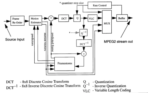
Figure 2.5 below, shows the main functional blocks within an standard MPEG2

encoder; motion estimator, several frame-stores, 8x8 DCT, quantizer (Q), entropy or VLC

encoder, inverse-quantizer (Q~), 8x8 IDCT, rate-control, and output-buffer.

*quantizer step size _{Rate Control}

Framne Motion + DCT Q VLC Buffer

-0'Re-Order Estimator _MUX

Source Input

S1 MPEG2 stream out

DCT

Framestores

DCT - 8x8 Discrete Cosine Transform Q -Quantization

DCT- -8x8 Inverse Discrete Cosine Transform Q-1 -Inverse Quantization

VLC -Variable Length Coding

(33)

The corresponding MPEG2 decoder is quite similar. It consists of a subset of the

encoder, with the addition of a VLC decoder. It should be noted that the motion estimator,

one of the most expensive functional blocks in the encoder, is not required by the decoder.

Therefore, the computational power required to implement an MPEG decoder is

substan-tially less than that required for an MPEG encoder. For this reason MPEG is characterized

as being an asymmetric algorithm where the requirements of the encoder are substantially

different from the decoder. A block diagram of an MPEG decoder is shown in Figure 2.6.

Quantizer step size

2MPEG2 Decoder Block Diagram Figure 2.6

(34)

Chapter 3 Recent Advances in Image Representation

As computing power has increased, the notion of what a digital image representation

should encompass has grown to be something more than just a compressed version of the

original. This chapter describes three recent approaches to image representation

under-taken at the Media Laboratory that have helped to inspire the work in this thesis.

3.1 Salient Stills

The Salient Still developed by Teodosio [28] is a good example of what can be done given

sufficient memory and processing time. The basic premise behind the Salient Still is that

one can construct a single image comprised of information from a sequence of images,

and that this single image contains the salient features of the entire sequence. The Salient

Still then has the ability to present not only contextual information in a broad sense (e.g.

the audience at a concert) but also the ability to provide extra resolution at specific regions

of interest or salient features (e.g. close up information of the performer at the concert). A

block diagram showing how a Salient Still is created is shown below.

(35)

The main algorithmic ideas to be gleaned from the Salient Still algorithm are;

. A single image is created by warping many frames into a common

space.

. The value of a pel at a particular point is the result of a temporally

weighted median of all the pels warped to that position.

- The motion model used to generate the warp is a 6 parameter affine

model derived by a Least Squares fit to the optical flow [6].

dx = ax+ b~x + cXy

(3.1)

d, = a,+ b x + cy

Some of the problems associated with salient generation are;

. Optical flow is particularly noisy near motion boundaries.

. Inaccurate optical flow fields result in an inaccurate affine model.

. The affine model is incapable of accurately representing motion other

than that which is parallel to the image plane.

3.2 Structured Video Coding

The "Lucy Encoder" described in Patrick McLean's Master's thesis "Structured Video

Coding" [18] explores what is possible if one already has an accurate representation of the

background. Footage from the 1950's sitcom "I Love Lucy" provided an easy means to

explore this idea for two reasons; first, the sets remained the same from episode to episode

and secondly, the camera motions used at the time were limited for the most part to pans.

Thus, construction of the background was a fairly easy process. All one had to do was

(36)

present. In addition to removing the actors, it was also possible to generate backgrounds

that were wider than the transmitted image, thus enabling the viewer to see the entire set as

opposed to the portion currently within the camera's field of view.

Having obtained an accurate background representation the next step was to extract

the actors. This proved to be no easy task. However, with some careful pruning and region

growing the actors were successfully extracted (along with a small amount of background

that surrounded them). Replaying the encoded footage then became a simple matter of

transmitting an offset into the background predictor and pasting the actors into the window

defined by this offset. McLean showed that if one transmitted the backgrounds prior to the

remaining foreground then it was possible to encode "I Love Lucy" with reasonable

qual-ity at rates as low as 64kbits/sec using Motion JPEG (M-JPEG1).

Several problems existed in the representation. Zooms could not be modeled as only

the motion due to panning was estimated. In addition, the segmentation sometimes did not

work as well as it should have, as either not all of an actor was extracted, or it was possible

to see where the actors were pasted back in by virtue of mismatch in the background.

However, these shortcoming are somewhat irrelevant as McLean demonstrated the more

important idea that the algorithm should generate a representation that was not based

solely on statistical models but one based on content. The representation now contained

identifiable regions that could be attributed to a distinct physical meaning such as a

"Lucy" region or a "Ricki" region.

1. Motion JPEG is a simple extension of JPEG for motion video in which each frame consists of a single JPEG com-pressed image

(37)

3.3 Layered Coder

More recently, work in the area of layered coding has been done by Wang, Adelson

and Desai [4], [30]. Along the same lines as the Salient Still and the Structured Video

Coder, the Layered Coder addresses the idea of modeling not just the background by

creat-ing a small number of regions whose motion is defined by a 6 parameter affine model.

These regions are transmitted once at the beginning of the sequence with subsequent

frames generated by compositing the regions together after they have been warped using

the 6 parameter models.

The regions are constructed over the entire sequence by fitting planes to the optical

flow field calculated between successive pairs of frames. Similar regions from each

seg-mentation are then merged to form a single region which is representative of its content for

the entire sequence.

As might be surmised this technique works best for scenes where rigid body non 3D

motion takes place. Another problem lies in the fact that the final regions have an error

associated with their boundaries due to the inaccuracies of the segmentation. Thus, when

the sequence is composited back together there tends to be an inaccurate reconstruction

near the boundaries. Finally, as only a single image is transmitted to represent each region

it turns out that closure (i.e. a value for every pel) cannot be guaranteed during the

com-positing stage after each region has been warped.

For all these reasons the layered coder does not generate pixel accurate replicas of the

frames in the original sequence for all but the simplest of scenes. However more

impor-tantly, even though a high Mean Square Error (MSE) may exist, the reconstructed images

look similar to the original. The error is now, not so much an error due to noise or

(38)

3.4 General Observations

The three representations described in this chapter share several things in common;

- Many frames are used to construct a single image representative of a

region in the scene.

. They construct this image using optical flow [6] to estimate interframe

motion.

- One or more 6 parameter affine models are used to represent the

inter-frame motion.

The techniques described above work well if one is attempting to model a simple

scene and can generate reasonable approximations to actual regions in a frame. However

if pixel accurate replication is required then, in general, the resulting images will not be

accurate due to geometric distortions introduced by the affine model's inability to

repre-sent 3D motion. Therefore given that an efficient reprerepre-sentation is paramount, if one

requires a geometrically accurate reconstruction or is modelling a sequence containing

significant amounts of 3D motion, then one should use a more accurate motion model in

addition to also including an error signal with the affine model to correct these distortions.

One final problem these methods face is that they rely on the accuracy of the motion

estimates generated by the optical flow algorithm. Optical flow attempts to determine the

velocity of individual pels in the image based on the assumption that the brightness

con-straint equation below holds.

d lum(x,y) = 0 (3.2)

(39)

This equation can be solved using a number of methods, the two most popular are

cor-respondence methods (which are essentially the same as block matching) and gradient

methods which attempt to solve the first order Taylor Series expansion of (3.2),

v

X

lum (x, y) + v 9alum (x, y) + a-lum (x, y) = 0 (3.3)

xax a~y a

over a localized region R [6]. In order for gradient based optical flow to work the

follow-ing assumptions are made;

. The overall illumination of a scene is constant,

. The luminance surface is smooth, . The amount of motion present is small.

When these assumptions are invalid optical flow fails to give the correct velocity

esti-mates. This is particularly true for;

. Large motions,

. Areas near motion boundaries,

. Changes in lighting conditions.

Thus for particularly complicated scenes involving lots of motion or lighting changes

the output from the optical flow algorithm will be inaccurate. Hence any segmentation

(40)

Chapter 4 Enhancing the Background Resolution

A theme common to the three representations described in the previous chapter was that

they all used more than one frame to construct a single representative image. The ability to

combine frames of video in this way can result in two benefits. First one can remove

fore-ground objects from the final image. Secondly, under certain conditions it may be possible

that the apparent resolution of the final image can be enhanced beyond that of the original

images.

This chapter concentrates on the second benefit, specifically, methods that increase the

sample density and resolution above that of the transmitted picture through the

combina-tion of several pictures sampled at different resolucombina-tions and times. The first benefit, that of

removing foreground objects from the final image, is the subject of the next chapter.

4.1 One Dimensional Sub Nyquist Sampling

Before examining resolution for images, it useful to examine a simpler one dimensional

problem that can later be extended into two dimensions for images. Consider the one

dimensional sequence x [n] shown below,

x [nJ

n

(41)

This sequence x [n] can be broken up into two sub nyquist sampled sequences; the

first consisting of even samples x, [n] and the second x, [n] of the remaining odd

sam-ples.

Figure 4.2

X,[n]

Sub nyquist sampled sequences, from odd and even Samples of Figure 4.1

The operations required to remove the even and odd samples from x [n] to generate

these sequences are described by the following formulae

X, [n] = (x [n] + (-1)x [n])

1

x, [n] = 1(x [n] - (-1)"x [n])

(4.1)

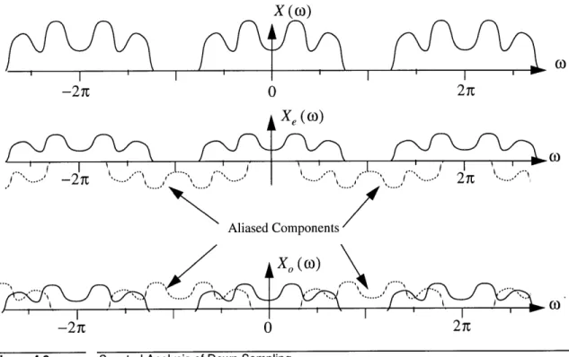
In the frequency domain these formulae correspond to the introduction of aliased versions

of the original sequence's spectrum,

Xe (o)) = I (x (o)) +X (-)

(4.2)

X0(o) = (X X

Furthermore, it easy to see that when these two sequences are added together the

(42)

AX (o) I -2 TE 0 2n Xe (0) Ahased Components X (o) -2 T 0 2 T

Figure 4.3 Spectral Analysis of Down Sampling

4.2 Enhancing Resolution Using Many Cameras

So far it has been shown that one can decompose a one dimensional sequence into two

sequences consisting of odd and even samples respectively. In addition, it was also shown

that the aliasing introduced during the creation of these two sequences is eliminated when

the two are recombined. Therefore, if one starts with two sequences, with the second

off-set half a sample period after the first, then it should be obvious to see how one could

cre-ate a sequence of twice the sampling density by zero padding and then addition.

If this concept is extended into two dimensions then it follows that four aliased input

sequences are required; odd rows/odd columns, odd rows/even columns, even rows/odd

columns, and even rows/even columns. Thus one could construct a four camera rig with

(43)

0

m~ ......... ---------- -... e e a .n... a a a a ... E0 Camera 1 M Camera 2 0 Camera 3 * Camera 4

Four Camera Rig for Doubling Spatial Resolution

Generally, such a system will not result in an exact doubling of the spatial bandwidth

as it relies on the assumption that frequency response of the camera is flat and contains

aliasing of only the first harmonic as shown below,

F (ox )

-27c -7t 7C 27c

f(x, y)

1/2 -1/4

Low pass response for no aliasing

-Ox, y

1/4 1/2

Desired Camera response for doubling resolution

Figure 4.4

21

-IV I

(44)

Real cameras are incapable of generating signals with the response shown in Figure

4.5 for three reasons;

. First, camera optics are not perfect and therefore they introduce a cer-tain amount of distortion into the image.

. Secondly, the sensors that form the camera chip are not infinitely small, they must have a significant finite area in order to reduce noise and also to minimize the magnitude of higher order aliased sidelobes.

. Third and finally, a real sensor is incapable of generating a negative response. Therefore it is impossible to implement f(x, y) as the response must be that of an all-positive filter.

Having deduced that it is impossible to obtain the desired response from practical sen-sors, one should determine how close the response of a practical sensor is to this ideal. Consider the 9 element ccd array shown in Figure 4.6,

b a. A b A B B Dark Im Clock A . Clock B -P+Islands Leslt bN-Type Lenselet Substrate age

Camera CCD Array (modified from Fig 2.22 in [5])

(45)

The sensors in this array have dimension a by b and are distributed on a rectangular grid with cells of size A by B. A common measure used to describe the geometry of the sensor array is the fill factor:

ab

AB (4.3)

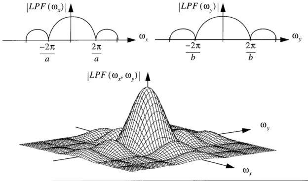
If the effect of the lenselets and other camera optical elements is temporarily ignored,

the frequency response due to the finite sensor area can be defined in terms of a separable function consisting of two sinc functions with nodal frequencies as shown in Figure 4.7. Notice that the response is low pass and that its width is dependent on the sensor size. Smaller sensors result in wider response than larger ones that filter out more of the higher

frequencies.

LPF (wo,) LPF(o)

a a b b

LP F (wx, (o,)|

Nx

Figure 4.7 Low pass frequency response due to finite sensor element size

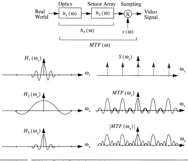
Reading the data from the ccd has the effect of multiplying the double-sinc frequency

(46)

X X X X X X Figure 4.8

X

A [0 X X B XT

4.4-X X X X 2 X X : 10 X X X X X X "OK X X X :X X X X X X X X X X X : 10( X X X X X X X X X X

Two dimensional pulse train

When one combines the effects of all these operations on the projected image one obtains the Modulation Transfer Function (MTF) which describes the behavior of the recording system. Following on from the previous examples the MTF for the ccd array in Figure 4.6 is shown below (NB only the x axis projection is shown for clarity).

LPF (o,) - )0 -2n -27c a A LPF (w,)

-2c

A -L 27c 2n A a n 2n A A

Modulation Transfer Function for a typical ccd array

46

Figure 4.9

Building the big picture : enhanced resolution from coding

Building the BIG Picture:

Enhanced Resolution from Coding

-V

Rftch

Building the BIG Picture:

Enhanced Resolution from Coding

Abstract

Building the BIG Picture:

Enhanced Resolution from Coding

Contents

List Of Figures

Chapter 1

Introduction

1.1 Motivation

1.2 The problem

1.3 Approach

>Full

Chapter 2

Image Coding Fundamentals

2.1 Representation

2.2

JPEG Standard [1]

2.2.1 Transform Coding

=j

f(x,y)cos

)

{F

up

m u.

mu,

Eu.

5

6

7

MEM.

MEE

NEu

0

ofl

1

2

3

-6

7-2.2.2 Quantization of Transform Coefficients

2.2.3 Entropy Coding

2.3 Frame Rate

2.4

MPEG Standards [2], [3]

2.4.1 Motion Estimation and Compensation

1

4567

2612718293313

X

I

SAD

(8GA,)

2.4.2 Residual Error Signal

Chapter 3

Recent Advances in Image Representation

3.1 Salient Stills

3.2 Structured Video Coding

3.3 Layered Coder

3.4 General Observations

X

Chapter 4

Enhancing the Background Resolution

4.1 One Dimensional Sub Nyquist Sampling

4.2 Enhancing Resolution Using Many Cameras

0

Nx

X

X

X

-2c

_f(x,y)cos

₎