Mesh Simplification in Parallel

READ THESE TERMS AND CONDITIONS CAREFULLY BEFORE USING THIS WEBSITE. https://nrc-publications.canada.ca/eng/copyright

Vous avez des questions? Nous pouvons vous aider. Pour communiquer directement avec un auteur, consultez la première page de la revue dans laquelle son article a été publié afin de trouver ses coordonnées. Si vous n’arrivez pas à les repérer, communiquez avec nous à PublicationsArchive-ArchivesPublications@nrc-cnrc.gc.ca.

Questions? Contact the NRC Publications Archive team at

PublicationsArchive-ArchivesPublications@nrc-cnrc.gc.ca. If you wish to email the authors directly, please see the first page of the publication for their contact information.

NRC Publications Archive

Archives des publications du CNRC

This publication could be one of several versions: author’s original, accepted manuscript or the publisher’s version. / La version de cette publication peut être l’une des suivantes : la version prépublication de l’auteur, la version acceptée du manuscrit ou la version de l’éditeur.

Access and use of this website and the material on it are subject to the Terms and Conditions set forth at

Mesh Simplification in Parallel

Langis, C.; Roth, Gerhard; Dehne, F.

https://publications-cnrc.canada.ca/fra/droits

L’accès à ce site Web et l’utilisation de son contenu sont assujettis aux conditions présentées dans le site LISEZ CES CONDITIONS ATTENTIVEMENT AVANT D’UTILISER CE SITE WEB.

NRC Publications Record / Notice d'Archives des publications de CNRC:

National Research Council Canada Institute for Information Technology Conseil national de recherches Canada Institut de Technologie de l’information

Mesh Simplification in Parallel

C. Langis, G. Roth and F. Dehne

December 2000

Copyright 2001 by

National Research Council of Canada

Permission is granted to quote short excerpts and to reproduce figures and tables from this report, provided that the source of such material is fully acknowledged.

*published in Proceedings of the 4th International Conference on Algorithms and Architectures for Parallel Processing (ICA3PP 2000),

MESH SIMPLIFICATION IN PARALLEL

CHRISTIAN LANGIS & GERHARD ROTH

National Research Council, Ottawa, Canada, {Christian.Langis,Gerhard.Roth}@nrc.ca FRANK DEHNE

School of Computer Science, Carleton University, Ottawa, Canada, frank@dehne.net

This paper presents a parallel method for progressive mesh simplification. A progressive mesh (PM) is a continuous mesh representation of a given 3D object which makes it possible to efficiently access all mesh representations between a low and a high level of resolution. The creation of a progressive mesh is a time consuming process and has a need for parallelization. Our parallel approach considers the original mesh as a graph and performs first a greedy graph partitioning. Then, each partition is sent to a processor of a coarse-grained parallel system. The individual mesh partitions are converted in parallel to the PM format using a serial algorithm on each processor. The results are then merged together to produce a single large PM file. This merging process also solves the border problem within the partition in a simple and efficient way. Our approach enables us to achieve close to optimal speedup. We demonstrate the results experimentally on a number of data sets.

1 Introduction

Mesh simplification is the process of approximating a high-resolution mesh by a coarser mesh with a lower triangle count. Traditional mesh simplification methods produce a coarser mesh but only at a single given resolution. By contrast, the Progressive Mesh (PM) representation [6] is a continuous resolution mesh. This category of representation stores in a compact fashion all resolutions between the lowest resolution (which is predefined) and the original high resolution mesh.

In a PM representation, an arbitrary mesh M is stored as a much coarser mesh M0 together with a sequence of vertex splits that indicates how to incrementally convert M0 back into the original mesh M = Mn. The PM representation of M thus defines a continuous sequence of meshes M0, M1, ..., Mn of increasing accuracy. The inverse of the vertex split is the edge collapse. With these two operations it is possible to create a mesh at any given resolution between the original high resolution mesh (M) and the lowest resolution mesh M0 (see Figure 1).

0 1 0 1 1 _... ) ˆ

(M =Mn  →ecoln− ecol → M  →ecol M

)

ˆ

(

...

M

M

M

M



 →





 →





 →



=

e d g e collapse vertex split v_{l v} l v_r v_r v_s v_s v_t

Since the simplification and refinement operations are very efficient, they can be performed in real-time. The PM representation has many applications. The most obvious is to use the representation for real-time level of detail (LOD) control for graphical rendering [10, 3]. Another application is the incremental transmission of a mesh on a network. The coarse M0 can be transmitted first, and the higher resolutions can be displayed incrementally as the vertex split operations are transmitted. Finally, the PM representation can be used to perform viewpoint dependent refinement [9].

While the display of the PM format is efficient, the creation of the PM sequence of edge collapses/vertex splits is more time consuming. At each step in the process it is necessary to choose which edge to collapse. This makes it necessary to compute the geometric error produced by each potential edge collapse and associate a cost with it. Once a cost is assigned to every edge, all potential edge collapses are sorted by cost. For large meshes this is a computationally intensive process.

Therefore, the creation of the PM sequence is a potential application for parallel processing. Our approach is to parallelize at the coarse-grained multiprocessor level by assigning different portions of the input mesh to different processes. We use a greedy graph partitioning algorithm to divide the mesh into disjoint subsets. Each mesh subset is sent to a “slave” processor where it is converted into the PM format using a serial algorithm. An important issue in such partition based parallel algorithms is the partition border problem. In this application, this problem manifests itself in the question of how to rejoin the PM representations at the border of the mesh partitions. We provide a solution to the partition border problem that is both simple and efficient. Our solution enables our parallelization approach to have a close to linear speedup, which is optimal. To our knowledge, no such parallel implementation of a continuous mesh creation algorithm exists in the literature.

The remainder of this paper is organised as follows. In Section 2, we give an overview of the parallel mesh simplification algorithm. In Section 3, we discuss the parallel implementation itself. Section 4 shows the results of our experimental performance analysis and we discuss the quality of our PM obtained in Section 5. Section 6 concludes the paper.

2 Parallel Mesh Simplification

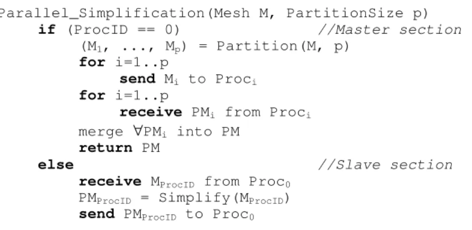
Our parallel implementation of the mesh simplification makes use of a standard serial algorithm for mesh simplification [6]. The approach for our parallelization is to partition the original high resolution mesh on a master processor and then to send each mesh partition to a slave processor. Each slave processor simplifies its associated mesh subset into a PM. Once this task is complete, each slave returns its

PM to the master processor which now merges them together to create a single PM file for the entire mesh. The following is the basic outline of our parallel algorithm: Parallel_Simplification(Mesh M, PartitionSize p)

if _{(ProcID == 0) //Master section}

(M1, ..., Mp) = Partition(M, p)

for i=1..p

send _{Mi to Proci} for i=1..p

receive _{PMi from Proci}

merge ∀PMi into PM

return PM

else //Slave section

receive _{MProcID from Proc0}

PMProcID = Simplify(MProcID)

send PMProcID to Proc0

Figure 2: Parallel Algorithm Pseudocode

2.1 Greedy Partition Method

The first step is to partition the mesh. We use is a simple greedy method where the graph partitioning problem is solved by accumulating vertices (or faces) in subsets when travelling through the graph. A starting vertex vs is chosen and marked. The

accumulation process is performed by selecting the neighbours of vs, then the

neighbours of the neighbours and so on until the subset has reached the required number of vertices. Then, other subsets are created the same way until the p-way partition is complete (e.g. each vertex is part of one subset). In the general case, such a p-way partition is built from p partial Breadth-First-Search traversals of the graph. The algorithm terminates when all vertices have been visited [2].

This simple greedy heuristic will yield acceptable partitions in much less time than more complicated methods. Furthermore, the algorithm can be made probabilistic if necessary [1]. It suffices to initialize it with a random vertex seed to generate different partitions for a same input graph. Figure 3 shows one 8-way partition example of this algorithm on a 3D mesh representing a duck [13].

The subsets being built may get blocked in the process before they reach full size. Then, two versions of the algorithm are possible: allow subset size imbalance or subset multi-connectivity. The former produces uneven subset sizes (workload on processors) and the latter produces bigger edge-cuts (more communication between processors). We chose the latter for better load balancing [4].

Figure 3: An exploded view of a 8-way partition of the 4K faces NRC Duck

2.2 Partition Border Problem

The main algorithmic problem for parallel progressive mesh simplification is the border problem. That is, how do we handle the triangles intersecting the border between different parts of the mesh as each part is processed in parallel on a different processor. Recall that the vertex set V of the mesh is partitioned into p disjoint subsets Vi whose union is V. Therefore, there are edges (and faces) between

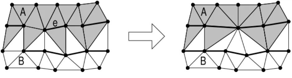
partition subsets (part of the edge-cut). Ideally, those edge-cut edges need to be dealt with just like subset edges. That is, during the parallel execution, at synchronisation points, there is an exchange of information between slave processors (potentially through the master processor) regarding the state of the mesh. Then, either of the neighbouring slave processors processes the shared edges using the edge information from the neighbours. This interdependence management scheme is costly but most applications are border-sensitive and require it. The graphs considered here are meshes representing 3D objects. The human eye accuracy sets the required quality level of processing. Hence, invisible degradation of the optimal result is allowed. In fact, we chose to avoid the border problem as long as possible. By not collapsing the edge-cut, one might expect to see the mesh separator in full resolution when the PM mesh is displayed at a coarse resolution. Fortunately, this is not the case. The edge-cut will be indirectly simplified along with any other edge. This phenomenon is shown in Figure 4.

e

A

B

A

B

Figure 4: Edge-cut Face Deletion

The partition snapshot represents the border between two subsets at some point during simplification. The two bold lines represent the link of each subset (the edge borders of subsets). The darker triangles belong to subset A and those in white belong to B. In this situation, the edge e from subset A will be collapsed. Note that, this edge has part of its neighbourhood in subset B. More precisely, e’s neighborhood has seven edges and six trianglesjoined to B by four vertices of B. However, if we simply force the collapse of e, the collapse affects only the structure (topology) of subset A. The neighbourhood part outside of A (vertices and edges and triangles of B) is left unchanged, topologically. It is only used to compute the best vertex position and the edge collapse cost for e. Following the collapse, two faces from A are deleted, including one from the edge-cut (between subsets). Therefore the parallel algorithm can simplify meshes as much as the sequential algorithm does, without the need for synchronisation steps or communications between processors.

3 Parallel Implementation

The code was written in C, using an MPI package for communication (more precisely, the free LAM-MPI [11]). The master processor partitions the mesh into p subsets. The partitioner will return a size |V| integer array. Each array cell corresponds to a mesh vertex and contains a subset ID ∈ [1..p] indicating the processor to which the vertex is assigned. The next step is to send that partition array to the slave processors. Then, all processors read the same mesh file into a

Mesh object exactly as in the sequential version. With the partition array at hand, the

slave processors build a working mesh structure of edges and faces which are either part of their partition subset or adjacent to it (surrounding edge-cut). Those edge-cut elements are included to address the border problem. Next, the slave processors build their edge collapse priority queues. In the parallel version, they do so with one extra condition: each edge must have both end-points in the slave processor’s vertex subset to allow a collapse. From that point on, the slave processor’s task remains the same as in the sequential program: it has a priority queue of edges to collapse.

After simplification, the slave processors must transmit their sub-results to the master processor for merging. This caused a technical difficulty. The data is now in the form of vectors, stacks and hashbags of vertices, edges and faces. Previously, the master sent an array of integers to the slaves. Now, the slave processors respond with arrays of more general objects. Our version of MPI does not support data communication other than standard data types. Therefore, we had to manually convert our arrays of objects to streams of standard data types and then back to objects. Once the data has been correctly communicated to the master processor and reconverted, the master contains p sets of four items sent by the p slaves: p hashbags of not deleted faces, p stacks of deleted faces, p vectors of collapsed edges and p vectors of new vertices. Those edge collapses were created independently. The master processor’s task is to synchronise them. For each collapse, an edge, a vertex and two faces are extracted from the data of one slave processor. The slaves collapse sets are visited in round-robin and their collapses are extracted one after another, from the best collapse performed to the most destructive one (See [4]). Another problem to be dealt with are duplicate faces. As mentioned, the subsets are sent to slave processors along with their surrounding edge-cut. Therefore, slave processors work independently on duplicate data. Consequently, all faces from the edge-cut will be replicated in the data returned by the slaves. For this reason, as the PM mesh is built, it must constantly be filtered for duplicate faces.

4 Performance Analysis

To evaluate the quality and performance of our implementation, we performed a series of tests on a network of Linux/Pentium 120Mhz/32Mb workstations (some were Pentium MMX 166Mhz). P0 was the master processor. We tested our program

with 2, 4, 8, and 16 processors connected to a 10Mbps Ethernet network. We ran these tests when most of the machines were idle. Unfortunately, there was no guarantee that the timings were not influenced by other users. This is clearly a very low cost and not state-of-the-art parallel processing platform. However, since we are mainly interested in measuring speedup, this platform was sufficient. Furthermore, if our method performs well on such a low cost platform, it will clearly be even better on more expensive and newer parallel machines.

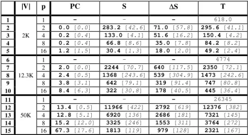
Our tests were conducted on two basic input meshes: the NRC Duck [13] and the Stanford Dragon [14]. We used various size meshes as input and processed each using various numbers of processors. The performace results are shown in Tables 1 and 2 below. Besides the total running time (T), we also measured the time to transfer the partition array to slave processors and read the input mesh on each processor (PC) as well as the PM computation time on each slave processor (S). Of particular importance is the load balance between slave processors. Recall that the mesh partitioning was obtained by a greedy partitioning algorithm as outlined in Section 2.1. We measured the difference between the slowest and fastest slave

processor with respect to S in order to see how thecomputational load is balanced between processors. For each input size |V| (the number of vertices in the input mesh) and number of processors p, we performed five test runs. All time values are in seconds. The bold numbers are averaged values and the italicised numbers in square brackets are their standard deviations. The blank lines no. 16 and 17 in Table 2 are caused by memory overflow. For meshes of such size, we needed to partition them among at least four processors so that each partition can fit into a processor’s memory. |V| p PC S ∆S T 1 1 - - - 618.0 2 2 0.0 [0.0] 283.2 [42.6] 71.0 [57.8] 295.6 [41.1] 3 2K 4 0.2 [0.4] 133.0 [4.1] 51.6 [16.2] 150.4 [4.2] 4 8 0.2 _[0.4] 66.8 _[8.6] 35.0 _[7.8] 84.2 _[8.2] 5 16 1.2 _[1.5] 30.4 _[1.3] 18.0 _[2.0] 49.2 _[2.4] 6 1 - - - 4774 7 2 2.0 _[0.0] 2244 _[70.7] 640 _[117.5] 2350 _[72.1] 8 12.3K 4 2.4 [0.5] 1368 [243.6] 539 [304.9] 1473 [242.6] 9 8 3.8 _[3.1] 642 _[79.1] 319 _[91.4] 747 _[80.8] 10 16 8.4 _[6.3] 322 _[30.8] 178 _[40.5] 445 _[36.4] 11 1 - - - 26345 12 2 13.4 _[0.5] 11966 _[422] 2792 _[619] 12376 _[382] 13 50K 4 12.8 [5.1] 6920 [136] 2686 [181] 7321 [145] 14 8 15.2 [12.0] 3325 [246] 1553 [311] 3764 [272] 15 16 67.3 _[17.6] 1813 _[119] 979 _[128] 2321 _[167]

Table 1: Parallel Simplification Statistics: NRC Duck

We now discuss our performance results in Tables 1 and 2. The main observation is that, despite the low cost communication network, the total time (T) observed for our method shows close to linear speedup. As expected, speedups are slightly lower for smaller data sets (|V|) and improve for larger data sets. The time for partitioning the data set (PC) increases with growing number of processors, as expected. What is very interesting to observe is that S often shows a more than linear speedup. How is this possible? The parallel algorithm does not explicitly collapse the edges that span the boundaries of the partition. The number of such edges increases with growing p. This effect does actually decrease the total work performed and, therefore, we can observe more than linear speedup. The load balancing of our method is measured in the ∆S column. Here, we observe that the load imbalance can be as high as 50%. Note, however, that finding an optimal partitioning of a mesh while minimizing the number of edges crossing boundaries is an NP complete problem. In our solution, we are using a greedy heuristic and for such a simple heuristic to be within a factor two of optimal is actually quite good.

We need to balance the time it takes to compute the partitioning (PC) versus the imbalance created (∆S) and the close to linear speedup for the total time T seems to indicate that the greedy heuristic used is a good compromise solution. With respect to the variances measured, we observe that they are fairly large. Clearly, the heuristic itself creates fluctuations but another important factor here is that we were performing our experiments in a multi-user environment. Furthermore, we observe that the variances for the total time (T) observed are considerably smaller than those for the other times measured.

|V| p PC S ∆S T 1 1 - - - 572 2 2 0.8 _[0.4] 265.4 _[2.3] 79.2 _[2.9] 307.2 _[3.1] 3 5.2K 4 1.0 [0.0] 132.2 [7.8] 42.2 [15.0] 171.6 [7.4] 4 8 1.4 _[0.8] 66.0 _[7.6] 31.0 _[11.1] 107.6 _[6.2] 5 16 2.6 _[2.7] 39.0 _[2.6] 25.4 _[2.5] 80.8 _[5.2] 6 1 - - - 3813 7 2 5.4 _[1.2] 1878 _[310] 560 _[362] 2079 _[308] 8 23K 4 6.0 [2.4] 949 [38] 328 [71] 1141 [39] 9 8 6.8 [3.6] 462 [22] 178 [36] 657 [28] 10 16 11.2 _[12.4] 233 _[13] 108 _[17] 425 _[12] 11 1 - - - 34811 12 2 52.8 _[28.4] 15617 _[452] 4057 _[161] 16577 _[429] 13 100.3K 4 68.5 _[56.5] 7158 _[70] 2086 _[126] 8211 _[174] 14 8 82.8 [1.8] 3449 [68] 1260 [127] 4427 [96] 15 16 162.8 _[3.1] 1776 _[75] 709 _[99] 2874 _[130] 16 1 - - - -17 2 - - - -18 198.3K 4 103 _[12] 29640 _[1367] 9483 _[2768] 32103 _[1638] 19 8 184 [20] 11338 [58] 3749 [307] 13714 [59] 20 16 369 [73] 5620 [13] 1873 [131] 8315 [353]

Table 2: Parallel Simplification Statistics: Stanford Dragon.

In summary, we conclude that the total time (T) observed for our method shows close to optimal linear speedup, even on a very low-cost, low-tech, communication network. We plan to test the method on other more advance machines, like a Cray T3E or IBM SP2, where we expect to obtain even better timing results.

5 Quality Analysis

Besides analyzing the runtime of our method, we also need to study the quality of the progressive mesh simplication obtained in comparison with the results of a purely sequential algorithm. Here, the main concern is about the edges that span the

boundaries of the partition. Everything else is processed with a sequential algorithm and is therefore of the same quality. With respect to the edges that span the boundaries of the partition, anomalies could appear in the obtained progressive meshes, along those boundaries. For example, the boundaries could become visible because there are “breaks” or different triangle densities along those boundaries. In Figure 4, process A collapses edge e whose neighbourhood contains four vertices from B. Furthermore, B collapses edges connected to those four vertices, indeed widening the extent of e’s neighbourhood (vertices) on B’s side. An edge collapse can be considered as the merge of a pair of vertices. Merging those four vertices with other vertices of B extends the neighbourhood of e on B’s side. Therefore, any vertex in B merged to one of those four neighbourhood vertices becomes part of e’s neighbourhood. However, as edge collapses are not communicated between slave processors, A will never be aware of it. Thus, the border edge neighbourhoods may include too few vertices from the adjacent vertex subsets. On the other hand, border edges remain as duplicates, and this may alleviate the problem. We examined progressive meshes obtained from using our algorithm on the NRC duck and other data and observed that, there are no visible breaks or inconsistency along the borders of our partitioning.

6 Conclusion

This paper presented a parallel algorithm for progressive mesh simplification. Our experiments show that the proposed method yields close to optimal speedup, even on a low-cost parallel platform. We presented a very simple solution for the problem of how to manage the border between different parts of the mesh partitioning. As mesh simplifications are becoming more important in 3D graphics, and parallel processing platforms are becoming more affordable (e.g. multi processor Pentium boards), parallel progressive mesh simplification methods will have an important role to play in such applications as parallel VR systems or the transmission of 3D models over networks.

7 Bibliography

1. Gilles Brassard, Paul Bratley. Fundamentals of Algorithms. Prentice-Hall, Chapter 10, 1996.

2. P. Ciarlet, F. Lamour. An Efficient Low Cost Greedy Graph Partitioning

Heuristic. CAM Report 94-1, UCLA, Department of Mathematics, 1994.

3. Andrea Ciampalini, Paolo Cignoni, Claudio Montani, Roberto Scopigno.

Multiresolution Decimation Based on Global Error. The Visual Computer 13

4. Christian Langis, Mesh Simplification in Parallel, MCS Thesis, Carleton University, Ottawa, Canada, 1999.

5. Brian Cort. An Implementation of a Progressive Mesh Simplification

Algorithm. Visual Information Technology Group, Institute for Information

Technology Group, NRC Canada, 1997.

6. Hugues Hoppe, Tony DeRose, Tom Duchamp, John McDonald, Werner Stuetzle. Mesh Optimization. Technical Report 93-01-01, Dept. Of Computer Science & Engineering, University of Washinton and SIGGRAPH 93 Proceedings, pp. 19-26. 1993.

7. M. Eck, TD. Rose, T. Duchamp, H. Hoppe, M. Lounsbery, W. Stuetzle.

Multiresolution analysis of arbitrary meshes. Computer Graphics Proceedings

Annual Conference Series, SIGGRAPH 95, ACM Press, pp.173-181, 1995. 8. Hugues Hoppe. Progressive Meshes, Microsoft Corporation and SIGGRAPH

96, 1996. http://www.research.microsoft.com/~hoppe/

9. Hugues Hoppe. View-Dependent Refinement of Progressive Meshes. Computer Graphics, SIGGRAPH 97 Proceedings, pp. 189-198, 1997.

10. Hugues Hoppe. Efficient Implementation of Progressive Meshes. Microsoft Corporation Report MSR-TR-98-02 and Computer & Graphics, 1998.

11. http://www.mpi.nd.edu/lam/

12. Patrick R. Morin. Two Topics in Applied Algorithmics. MCS thesis, Carleton University, 1998.

13. http://www.vit.iit.nrc.ca/~roth