Application of multivariate control system design methodologies to robust beam control of a space-based laser

Application of Multivariable Control System

Methodologies to Robust Beam Control of

a Space-Based Laser

Kelly Douglas Hammett B.S., Aerospace Engineering

University of Oklahoma (1988)

SUBMITTED TO THE DEPARTMENT OF AERONAUTICS AND ASTRONAUTICS IN PARTIAL FULFILLMENT OF THE

REQUIREMENTS FOR THE DEGREE OF MASTER OF SCIENCE

at the

MASSACHUSETITS INSTITUTE OF TECHNOLOGY June 1991

) Kelly Douglas Hammett, 1991. All rights reserved.

The author hereby grants to MIT and the C.S. Draper Laboratory, Inc. permission to reproduce and to distribute copies of this thesis document in whole or in part.

Signature of Author

/ Department of Aeronautics and Astronautics May 10, 1991 Certified by

U

IF ,., //

Dr. John R. Dowdle Section, C.S. Draper Lab Technical Supervisor Certified by

Accepted by

Michael Athans SProfessor of Electrical Engineering Thesis Supervisor No

Professor IWld Y. Wachman ChahirimFn taFraCr duate Committee MASSACHiUSETfS i NSTITUTE OF TEC•.""' nY"

JUN

'

1991

Design

Application of Multivariable Control System Design

Methodologies to Robust Beam Control of

a Space-Based Laser

by

Kelly Douglas Hammett

Submitted to the Department of Aeronautics and Astronautics

on May 10, 1991, in partial fulfillment of the requirements

for the degree of Master of Science in Aeronautics and Astronautics

Abstract

The complexity of large-scale dynamic systems provides a challenging proving

ground for modern control system analysis and design techniques. High plant

dimensionality inherent in large-scale systems can lead to breakdowns in numerics of

state-space algorithms or intolerably long computational times, necessitating use of model

reduction techniques. Reducing plant order consequently introduces unmodeled dynamics

into the system, which must then be accounted for via stability and performance robustness

considerations. A design framework is adopted herein which allows stability robustness to

be guaranteed via unstructured uncertainty representation and the Small Gain Theorem, and

performance robustness to be independently verified. The applicability of modem

multivariable controller design techniques to large-scale systems is demonstrated by

synthesis of robustly stable H

compensators for a space-based laser forebody using reduced order models. Performance

goals are expressed in terms of both allowable 2-norms and root-mean-square values of

line-of-sight and segment phasing errors, and an evolutionary process leads to a final

controller design. First, ideally performing but non-robust unconstrained bandwidth H

and H. designs are presented which illustrate the danger of ignoring unmodeled

high-frequency dynamics. Then robustly stable but poorly performing reduced bandwidth H

and H., designs are derived, achieved via constant penalizing of the system control at all

frequencies. Next, frequency-dependent penalty of the errors/controls leads to H

loop-shaping designs, which yield superior closed-loop performance and stability

robustness. Issues relating to digital implementation of continuous-time controllers are

addressed, a study of reduced-order compensators is performed, and the final design is validated via time domain simulation and steady-state covariance analysis. Finally, performance robustness issues and effects of parametric uncertainty on open-loop system model natural frequencies are addressed.

Thesis Supervisor: Professor Michael Athans Title: Professor of Electrical Engineering, M.I.T. Technical Supervisor: Dr. John R. Dowdle Title: Chief, Flight Systems Section

Acknowledgements

I would like to express my appreciation to the Charles Stark Draper Laboratory and the United States Air Force for providing me the opportunity to pursue graduate level education at the Massachusetts Institute of Technology. Over the course of my two years at MIT, both the financial and personal support from these two organizations have proven to be tremendous. Several individuals played key roles in helping me to even get here, most notably Dr. Dave Burke from CSDL and Major David Alkove, USAF.

I would also like to acknowledge a strong sense of gratitude and respect for Dr. John R. Dowdle for both the depth and breadth of his technical expertise, and for the extreme and patient willingness with which he shared that expertise. His personal concern and sense of humor made my stint as a graduate student at MIT and CSDL enjoyable as well as intellectually rewarding. I simply could not have asked for a better supervisor.

My MIT thesis advisor, Professor Michael Athans, constantly pushed me toward a better physical understanding of the issues involved in this thesis and in multivariable control in general, and for this furthering of my education I owe a debt of appreciation.

My thanks also to Dr. Brent Appleby, Dr. Karl Flueckiger, Mr. Tim Henderson, Mr. Robert Regan, and Mr. Duncan McCallum all of CSDL for assisting me through a number of problematic technical challenges encountered along the way.

I would like to thank my parents for providing a fundamental base upon which my education could be built, and for their assistance in helping me complete my undergraduate education which enabled me to reach the point where I am now.

Finally, and most importantly, I would like to thank my wife, Kellie, for leaving behind all that she knew to join me on this voyage of higher learning and cultural adjustment. Her patience while I devoted the bulk of my time to my studies has been

greatly appreciated, and her sacrifices have provided constant incentive to make the most out of my educational opportunities at MIT. I therefore dedicate this thesis to her.

This thesis was prepared at The Charles Stark Draper Laboratory, Inc., under Independent Research and Development funding. Publication of this report does not constitute approval by the Draper Laboratory or the Massachusetts Institute of Technology of the findings or conclusions contained herein. It is published solely for the exchange and stimulation of ideas. I hereby assign my copyright of this thesis to The Charles Stark Draper Laboratory, Inc., Cambridge, Massachusetts.

Contents

List of Figures...8

List of Tables...

13

Notation and Abbreviations ... ...

14

1 Introduction ...

17

1.1 Background ... 17

1.2 SBL System Concept ... 18

1.3 Problem Description...19

1.4 Discussion ... 21

1.5 Thesis Contributions and Outline... 22

2 Problem Statement ...

25

2.1 Problem Summary...25

2.2 The SBL Model... 25

2.2.1 Physical System Description ... 25

2.2.2 Mathematical Model ... 30

2.3 Performance Specifications...35

3 Open-Loop System Analysis

...

39

3.1 Introduction ... 39

3.2 Nominal Stability ... ... ... 39

3.3 Multivariable Transmission Zeros ... 43

3.4 Singular Value Frequency Response ... 48

3.4.1 Definitions... 48

3.4.2 Importance of Singular Values to LTI Systems...49

3.4.3 Open-Loop Singular Value Frequency Responses...54

4 Model Reduction ...

59

4.1 Introduction ... 59

4.2 Controllability/Observability Issues ... 59

4.4 Application of Model Reduction Techniques ... 62

5 A Methodology for Robust Control System Synthesis...69

5.1 Introduction ... 69

5.2 Stability Robustness via the Small Gain Theorem ... 69

5.3 Compensator Design Techniques... 73

5.3.1 Introduction ... 73

5.3.2 H2 Optimal Control ... ... 74

5.3.3 H.I Optimal Control ... 76

5.3.4 Loop-Shaping Techniques ... ... 78

6

The Design Plant Model...

... 81

6.1 Introduction ... ... 81

6.2 Error Vector Formulation and 2-Norm Bounding ... 82

6.3 Disturbance Vector Formulation and 2-Norm Bounding ... 85

6.4 Requirements Analysis via H. Design ... 87

6.4.1 Procedure ... 87

6.4.2 Segment Phasing Sensor Configuration Study ... 87

6.4.3 Disturbance Environment Scenario... 90

6.5 Augmentation of the Multiplicative Error Block ... 93

7 Compensator Designs ...

...

...

99

7.1 Introduction ... ... 99

7.2 Nominal Performance (Unconstrained Bandwidth) Designs ... 100

7.3 Robust Designs ... ... 108

7.4 Loop-Shaping Designs... ... 116

7.4.1 Introduction ... ... 116

7.4.2 Weighted-Error H2 Design...116

7.4.3 Weighted-Control H.I Design ... 127

8 Implementation/Validation Issues ...

137

8.1 Introduction ... ... 137

8.2 Digital Implementation Issues ... ₁₃₇

8.3 Reduction of Compensator Order... 141

8.4 Design Simulation ... 145

8.4.2 Stochastic Time-Domain Simulation ... 146

8.4.2 Deterministic Sinusoidal Simulation ... 158

8.5 Performance Robustness and Effects of Open-Loop Natural Frequency Parametric Uncertainty ... 163

9 Conclusions...

170

9.1 Summary ... ... 170

9.2 Conclusions...172

9.3 Recommendations for Further Research ... 173

List of Figures

1.1 SBL Forebody ... ... 18

1.2 Primary Mirror Misalignment and Segment Phasing Error... ... 20

2.1 SBL Beam Expander Assembly ... 26

2.2 Outer Segment Position Actuator Configuration ... 27

2.3 BEA RTZ Coordinate Axis System. ... 28

2.4 BEA XYZ Coordinate Axis System...29

2.5 Segment Phasing Sensor Locations... ... ... 30

2.6 Block Diagram Representation of Open-Loop Plant (3-Block Form) ... 31

2.7 Block Diagram Representation of Open-Loop Plant (1-Block Form) ... 32

2.8 Equal Peak Intensity Attenuation Contours... ... 37

3.1 Open-Loop Pole Plot (Note Scale Differences) ... 43

3.2 Closed-Loop Transfer from u to y (with sensor noise present) ... 46

3.3 Open-Loop Multivariable Transmission Zeros...47

3.4 Open-Loop Multivariable Transmission Zeros (Close-up About the Origin) ... 47

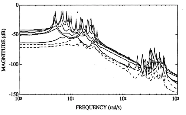
3.5 Open-Loop Singular Value Frequency Response from Controls to Outputs... ... 55

3.6 Open-Loop Max. Singular Value Frequency Response from Combined Controls and Disturbance Torques to All Errors ... ... 55

3.7 Open-Loop Max. Singular Value Frequency Response from Disturbance Torques to All Errors... 56

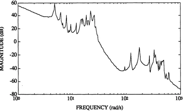
3.8 Open-Loop Transfer from Disturbance Torques to Segment Phasing Errors.... ... 57

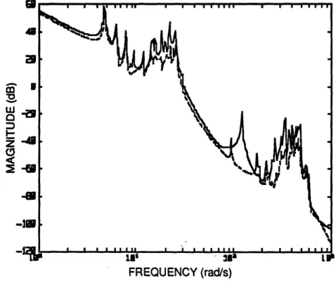
3.9 Open-Loop Transfer from Disturbance Torques to Line-of-Sight Errors...58

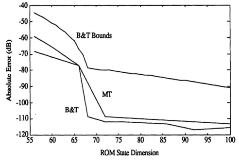
4.1 B&T ROM Additive Error.Upper Bounds. ... ... 63

4.2 Infinity Norms of Computed Additive Errors vs ROM Order...64

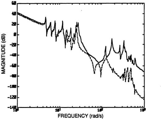
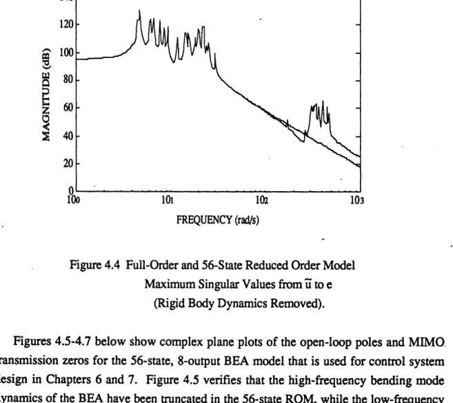
4.4 Full-Order and 56-State Reduced Order Model

Maximum Singular Values from ii to e (Rigid Body Dynamics Removed)...66

4.5 Open-Loop Pole Plot (56-State Model) ... 67

4.6 Open-Loop Multivariable Transmission Zeros (56-State Model) ... 68

4.7 Open-Loop Multivariable Transmission Zeros (56-State Model, Close-up About the Origin) ... 68

5.1 Topology for the Small Gain Theorem ... 70

5.2 ROM with Multiplicative Modeling Error...71

5.3 Augmented Plant (3-Block Form) ... ... 71

5.4 Closed-Loop Transfer Function ... 72

5.5 Weighted Open-Loop 2-Block Model... 79

6.1 Nominal Open-Loop 2-Block System... .... 81

6.2 Closed-Loop System with Scaled Error Vector ... 83

6.3 Closed-Loop System with Scaled Disturbance and Error Vectors... .... 86

6.4 Requirements Analysis Sensor Configurations ... ... 88

6.5 y= 1 Versus ( 11 dT 112 , II 112 ). ... ... ... 89

6.6 Achievable Performance Versus ( II dT 112 , II 0 112 (Sensor Configuration 1) ... ...90

6.7 ROM with Multiplicative Modeling Error...93

6.8 Actual Open-Loop Plant ... 93

6.9 Multiplicative Modeling Error at the Plant Output. ... ... 94

6.10 ROM with Scaled Error Block...95

6.11 Augmented Plant with Scaled Error Block ... 96

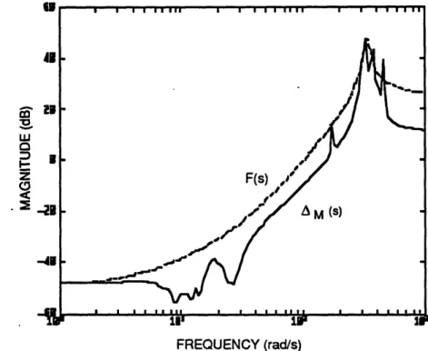
6.12 Plant Output Multiplicative Modeling Error and Bounding Transfer Function, F(s). ... _{.... 96}

7.1 Open and Closed-Loop Transfer From All Disturbances to All Errors (T22) (Unconstrained Bandwidth Designs) ... 101

7.2 Max. Singular Value Closed-Loop Transfer from Torque Disturbances to Segment Phasing Errors (T22 11) (Unconstrained Bandwidth Designs)...102

7.3 Max. Singular Value Closed-Loop Transfer from Sensor Noise to Segment Phasing Errors (T22 12) (Unconstrained Bandwidth Designs)...103

7.4 Max. Singular Value Closed-Loop Transfer from Torque Disturbances to Line-of-Sight Errors (T2221) (Unconstrained Bandwidth Designs)...103

7.5 Max. Singular Value Closed-Loop Transfer from Sensor Noise to

Line-of-Sight Errors (T2222) (Unconstrained Bandwidth Designs) ... 104

7.6 Closed-Loop Transfer About AM (T11)

(Unconstrained Bandwidth Designs)... ... 105 7.7 Unconstrained Bandwidth Compensator Maximum

Singular Value Frequency Responses... ... 106

7.8 Complementary Sensitivity at Plant Output

(Unconstrained Bandwidth Designs)...108

7.9 Open and Closed-Loop Transfer From All Disturbances

to All Errors (T

2) (Robust Designs)...10

7.10 Closed-Loop Transfer About AM (T11) (Robust Designs) ... 110

7.11 Max. Singular Value Closed-Loop Transfer from Torque Disturbances

to Segment Phasing Errors (T

2

1) (Robust Designs) ... 111

7.12 Max. Singular Value Closed-Loop Transfer from Sensor Noise

to Line-of-Sight Errors (T22

) (Robust Designs)...12

7.13 Max. Singular Value Closed-Loop Transfer from Torque Disturbances

to Line-of-Sight Errors (T22

7.14 Max. Singular Value Closed-Loop Transfer from Sensor Noise

to Line-of-Sight Errors (T2222

) (Robust Designs)...

113

7.15 Robust Compensator Maximum Singular Value Frequency Responses ... 114

7.16 Complementary Sensitivity at Plant Output (Robust Designs) ....

... 115

7.17 Closed-Loop Transfer from All Disturbances to All Errors (T22)

(Weighted-Error H2 Design, wb

=

0.1 rad/s) ... 119

7.18 Closed-Loop Transfer from All Disturbances to All Errors (T2

)

(Weighted-Error H

Design, cb

=

10 rad/s) ... 120

7.19 Error Shaping Filter Frequency Response

(Weighted-Error H

Design, cb = 2 rad/s)...121

7.20 Closed-Loop Transfer from All Disturbances to All Errors (T22)

(Weighted-Error H

Design, cob

=

2 rad/s) ... 121

7.21 Closed-Loop Transfer about AM (T

)

(Weighted-Error H

=

2 rad/s) ...

... 122

7.22 Max. Singular Value Closed-Loop Transfer from Torque Disturbances

to Segment Phasing Errors (T2211)

7.23 Max. Singular Value Closed-Loop Transfer from Sensor Noise to Segment Phasing Errors (T22 12)

(Weighted-Error H2 Design, aob = 2 rad/s)... 123

7.24 Max. Singular Value Closed-Loop Transfer from Torque Disturbances

to Line-of-Sight Errors (T2221)

(Weighted-Error H2 Design, ob = 2 rad/s) ... 124

7.25 Max. Singular Value Closed-Loop Transfer from Sensor Noise to Line-of-Sight Errors (T₂₂₂₂)

(Weighted-Error H2 Design, ob = 2 rad/s)... 124

7.26 H2 Loop-Shaped Error Compensator Maximum Singular Values ...125

7.27 Complementary Sensitivity at Plant Output

(Weighted-Error H2 Design, cob

=

2 rad/s) ... 126

7.28 Control Shaping Filter Frequency Response...

... 130

7.29 Closed-Loop Transfer from All Disturbances to All Errors (T22)

(Weighted-Control H. Design). ... 130

7.30 Closed-Loop Transfer about AM (T

)

(Weighted-Control H. Design). ... 131

7.31 Max. Singular Value Closed-Loop Transfer from Torque Disturbances to Segment Phasing Errors (T2211)

(Weighted-Control H. Design). ... 132 7.32 Max. Singular Value Closed-Loop Transfer from Sensor Noise

to Segment Phasing Errors (T2212)

(Weighted-Control H.•Design). ... ... 132 7.33 Max. Singular Value Closed-Loop Transfer from Torque Disturbances

to Line-of-Sight Errors (T_{222 1})

(Weighted-Control H. Design). ... ... 133 7.34 Max. Singular Value Closed-Loop Transfer from Sensor Noise

to Line-of-Sight Errors (T₂₂₂₂)

(Weighted-Control H. Design). ... 133 7.35 H. Loop-Shaped Control Compensator Maximum Singular Values ... 134 7.36 Complementary Sensitivity at Plant Output

(Weighted-Control H.* Design) ... 135 8.1 Open-Loop System with C-T Compensator...139 8.2 Open-Loop System with D-T Equivalent Compensator...139

8.3 Hoo Loop-Shaped Control Compensator Hankel Singular Values

versus State Dimension ... 142

8.4 Closed-Loop Transfer from-AN Disturbances to All Errors (T22) (72-State Com pensator)... .... 143

8.5 Closed-Loop Transfer from All Disturbances to All Errors (T22) (73 and 80-State Compensators) ... 143

8.6 73 and 80-State Ho, Loop-Shaped Control Compensator Max Singular Value Frequency Responses...144

8.7 Closed-Loop Transfer about AM (T₁₁) (73-State Ho Loop-Shaped Control Compensator) ... 145

8.8 Stochastic Torque Disturbance 1 Time Response... 152

8.9 Stochastic Torque Disturbance 2 Time Response...152

8.10 Open-Loop Position 14 Segment Phasing Error Time Response ... 154

8.11 Closed-Loop Position 14 Segment Phasing Error Time Response...54

8.12 Open-Loop LOS X Error Time Response ... ...155

8.13 Closed-Loop LOS X Error Time Response ... 156

8.14 Petal 1 Radial Actuator Time Response... 157

8.15 Petal 1 Longitudinal Actuator Time Response ... 157

8.16 Open-Loop Max. Segment Phasing Error Time Response ... 159

8.17 Open-Loop LOS Y Error Time Response ... 160

8.18 Closed-Loop Segment Phasing Error Time Responses ... 161

8.19 Closed-Loop LOS Error Time Responses ... ... 161

8.20 Closed-Loop Pole-Plot... 162

8.21 Perturbed System Plant Output Multiplicative Errors and Bounding Transfer Function Frequency Responses ... 165

8.22 Closed-Loop Transfer about AM (T11) (Perturbed Open-Loop Natural Frequency Systems)...166

8.23 Closed-Loop Transfer from All Disturbances to All Errors (T22) (5% More Stiff Open-Loop System) ... ... 167

8.24 Closed-Loop Transfer from All Disturbances to All Errors (T22) (5% Less Stiff Open-Loop System) ... 168

8.25 Closed-Loop Transfer from All Disturbances to All Errors (T22) (108-State Truth Open-Loop System)...169

List of Tables

6.1 Aftbody Slew Manuever Requirements ...

91

8.1 Steady-State Covariance Analysis Results

Notation and Abbreviations

r complex-valued vector

Cn _{vector space of complex-valued vectors with n elements}

r(t) real-valued vector signal R complex-valued matrix

rT, RT transpose of the vector r, matrix R

rH, RH _{Hermitian (complex-conjugate transpose) of the vector r, matrix R} tr (R) trace of the matrix R

R-1 inverse of the matrix R

R> 0 the matrix R is positive definite R > 0 the matrix R is positive semi-definite

ki(R) ith eigenvalue of the matrix R

Won undamped natural frequency associated with the ith eigenvalue

C damping ratio of the ith eigenvalue oi(R) ith singular value of the matrix R

ol(R) _{maximum singular value of the matrix R} G(s) open-loop transfer function

T(s) closed-loop transfer function K(s) compensator transfer function A(s) uncertainty block transfer function

So(s) output sensitivity transfer function

Co(s) output complementary sensitivity transfer function

x vector of system state variables

z input vector to the uncertainty block w output vector to the uncertainty block

d input vector containing all exogenous disturbances signals (disturbances, sensor noises, and reference inputs)

e performance or error vector (to be kept small)

u control input vector y measured output.vector

dT disturbance torque vector

uvector of combined disturbance torques and control inputs 0 additive sensor (measurement) noise vector

ar, ar2 root-mean-square value, variance of stochastic vector signal r Ilrllp pth-norm of the vector r

IIG(s)Ilp pth-norm of the transfer function G(s)

H2 the subspace of complex-valued functions analytic and with bounded 2-norms in the complex right-half plane

Hoc the subspace of complex-valued functions analytic and with bounded infinity-norms in the complex right-half plane

Y upper bound on gamma-iteration infinity-norm achievable performance p scalar control weight

rsteady-state covariance matrix of stochastic vector signal r ODr power spectral density of stochastic vector signal r

SBL space-based laser HEL high-energy laser

BEA beam expander assembly LQG Linear Quadratic Gaussian DPM Design Plant Model LOS line-of-sight

R'IZ radial-tangential-longitudinal RMS root-mean-square

GEP generalized eigenvalue problem LTI linear time-invariant

SISO single-input, single-output MIMO multi-input, multi-output

BIBO bounded-input, bounded-output SVD singular value decomposition FOM full-order model

ROM reduced-order model

B&T balance and truncate (model reduction algorithm) MT modal truncation (model reduction algorithm) HSV Hankel singular value

SGT Small Gain Theorem

dB decibel

C-T continuous-time D-T discrete-time

CHAPTER 1

Introduction

1.1 Background

Following President Ronald Reagan's launching of the Strategic Defense Initiative (SDI) in 1983, great interest was generated in the United States' research and development community toward viable system concepts for protecting this country from the threat of weapons delivered through outer space. The prime motivation for developing. such a defense system lay in the large stockpile of nuclear warheads amassed by the Soviet Union in the 1970s, and the arsenal of intercontinental ballistic missiles (ICBMs) maintained to deliver them. The purpose of SDI was to research and develop systems that could somehow render ICBMs harmless before they struck their ground targets, preferably while the warheads were still outside the earth's atmosphere. During the course of the mid and late 1980s, several widely different concepts to meet this purpose were considered, and one that generated great interest and enthusiasm was that of the space-based laser (SBL). At the time of SDI's inception however, a number of critical technologies required for implementation of the space-based laser concept were lacking. These undeveloped technologies included mirror manufacturing techniques, power generation methods, and signal processing/control system algorithms and hardware, to name but a few. The widespread and intense research effort of the mid and late 1980s led to progress in many of these areas, but realizable and effective control system design for space-based lasers remains a topic of current research. It is this topic that is pursued in this thesis.

1.2 SBL System Concept

Before proceeding further, a brief and somewhat general description of an SBL physical system concept and relevant terminology is presented to facilitate discussion. For purposes of this study, the space-based laser can be visualized as consisting of two parts, the forebody and the aftbody. The aftbody consists of the satellite platform, and contains all necessary equipment for orbital station-keeping and satellite attitude control. In addition, the SBL aftbody contains the mechanisms required for generation of the high-energy laser (HEL) beam, and adequate optical components for transfer of the beam to the SBL forebody. The forebody of the SBL houses the beam expander assembly (BEA), which consists of a large, deformable primary mirror attached to a rigid bulkhead support, a much smaller and stiffer secondary mirror, a metering truss to maintain relative positions of the two mirrors, and all necessary sensors and actuators for accomplishing required control functions. The BEA points, magnifies, and focuses the HEL beam generated in the aftbody as necessary to meet various mission requirements. Figure 1.1 below shows the SBL forebody. Further details concerning the SBL are provided along with the description of the system model in Chapter 2.

1.3 Problem Description

Simply stated, the objective of the space-based laser is to place sufficient energy on a distant, rapidly moving target for a long enough duration to accomplish one of several envisioned tasks, all having to do with negation of the threat posed by the target. The control aspects of the SBL problem are numerous and formidable. They encompass several tasks, including high-energy laser beam generation and propagation, satellite platform orbital and attitude control, and acquisition, tracking, and pointing (ATP) functions.

One of the most challenging areas of the SBL control problem is that of beam control. Beam control consists of two main functions: beam pointing and wavefront control, both of which involve steerable and/or deformable optical components. Beam pointing involves placing and maintaining the HEL beam on a desired aimpoint, while wavefront control deals with maintaining a spatially coherent and in phase sequence of light waves.

Wavefront control is the most difficult of the two functions, for it involves extremely precise shape control of the entire SBL primary mirror, which is envisioned as having a diameter of ten meters or more. Due to the large size of this primary mirror, current manufacturing and deployment scenarios call for the primary mirror to be composed of several mirror segments or petals. Longitudinal misalignments of the mirror segment edges result in differences in optical path length for various parts of the laser beam, thereby inducing wavefront phasing errors and potentially destructive interference (see Figure 1.2). Preventing degradation of laser beam quality due to these separations is referred to as the segment phasing aspect of the wavefront control problem [1].

PRIMARY MIRROI SEGMENT EDGE MISALIGNMENT R WAVEFRONT PHASING

Figure 1.2 Primary Mirror Misalignment and Segment Phasing Error.

Beam pointing is also a complex control task, involving boresight measurements, autoalignment, and beam jitter control functions [2]. Roughly speaking, boresighting involves placing the laser beam on a selected aimpoint, and jitter control involves keeping it there in the presence of disturbances, such as vibrations transmitted through the SBL bulkhead. Autoalignment refers to the static coordination of the various laser beam steering components on the fore and aftbodies of the SBL in order to assure smooth transfer of the

HEL beam.

This thesis addresses the problem of simultaneously maintaining tight beam jitter control and minimizing the effects of destructive interference induced via segment phasing. The control algorithms considered are all of a centralized nature, meaning that all sensory data is processed and control authority will be generated from one central computer. Shape control of the primary mirror for the purpose of wavefront control is not addressed, nor are station-keeping and attitude control issues considered. These three control functions will fall under the jurisdiction of actuators different from those used for the beam jitter and segment phasing problems.

1.4 Discussion

Control system synthesis for "large-scale" uncertain systems such as the SBL forebody described above poses many challenges to the control engineer. Typical large-scale systems, such as flexible space structures, often possess very little damping, placing the open-loop poles of such systems close to the s-plane imaginary axis, and thus close to open-loop instability. The presence of a large number of open-loop poles near the instability boundary can lead to difficulties in obtaining closed-loop stability and/or stability robustness. Also, structural models of large-scale systems typically possess dynamics encompassing a large range of open-loop natural frequencies. Large magnitude differences between open-loop poles leads to ill-conditioned system model matrices, making certain numerical computations difficult. Truncation of high frequency dynamics and/or construction of slow/fast control loops may therefore be required.

The size and complexity of large scale systems pose additional problems for the designer. State-space models of large-scale systems are typified by matrices of very large dimensions, hence the categorization as "large-scale". The sheer bulk of such models can cause difficulties with the numerics of solution algorithms, in addition to requiring excessive amounts of valuable computational time and resources. .Also, model-based control system design methodologies prescribe high-order compensators for high-order plants. Compensators of such large order are cumbersome to implement due to excessive data processing time requirements, and model reduction methods must therefore be used to obtain simpler realizations.

Approximating the plant with reduced-order models introduces errors into the system, which must then be considered in the design process. Of course, as is necessary for all realistic design problems, the control system design engineer must deal with unpredictable disturbances acting on the system and with unintentional modelling errors or uncertainties, such as parametric uncertainty (uncertainty in knowledge of plant parameters). These considerations lead to robustness of stability and performance issues which the designer must address.

Finally, implementation issues must be examined to assess the practicality of the design being considered. Centralized versus decentralized control authority, determination of allowable order of the compensator and methods of implementation, and software or hardware limitations are just some of the issues to be examined.

Fortunately for the control system engineer, a variety of procedures (pole-placement, LQG/LTR, H2, H., j±-synthesis, L1, etc.) [3] are currently available to help the designer

meet specified performance goals. However, not all of these methods are applicable to any given problem. The control system designer must select the method which yields the best results for the given problem and design objectives. This, then, suggests the need to apply the applicable algorithms to the given problem and compare results to identify the "best"

controller for the stated performance goals. For typical large-scale system examples, once

an appropriately sized reduced-order model is obtained, the synthesis procedures can be applied to design the various controllers, and closed-loop performance and robustness can

be evaluated.

1.5 Thesis Contributions and Outline

Past efforts related to the mirror control problem have employed both single input,

single output (SISO)

[4,5]

and modern multivariable design techniques [1,6]. SISO

approaches attempt to model the system dynamics as a series of independent SISO

systems, and ignore the potentially significant effects of dynamic coupling between various

input-output pairs. Multivariable approaches, on the other hand, allow coupling between

inputs and outputs to be fully represented in system models, and therefore yield more

accurate results. Since typical large-scale systems are represented by high-order models

with multiple sensors and actuators that inevitably possess some degree of dynamic

coupling, multivariable design methods are clearly more appropriate for this type of

problem. In [1] the LQG/LTR approach was applied to the segment phasing problem,

demonstrating the applicability of this multivariable design method to the problem, but

failing to achieve desired performance results. In [6] a preliminary analysis addressing the

applicability of the pt-synthesis design procedure to the beam jitter disturbance rejection

problem was considered.

This thesis carries out a comprehensive multivariable feedback controller synthesis

procedure for the combined SBL BEA segment phasing and beam jitter control problems.

Details and results of application of H

optimal, H. optimal, and H

design methodologies [7] are presented, and the trade-offs resulting from use of the various

design techniques are thoroughly illustrated. The use of model reduction techniques to

obtain an appropriately sized design model, in conjunction with use of the Small Gain Theorem to guarantee stability robustness to the truncated dynamics, is also shown. Additionally, a technique for requirements analysis via H. optimization is introduced. Following compensator design, numerous practical implementation issues are addressed, including digital implementation of continuous-time compensators, reduction of compensator order, design validation via simulation and covariance analysis, and effects of open-loop natural frequency parametric uncertainty. Finally, performance robustness of the final design selected to unmodeled dynamics is verified.

Following this introductory chapter, this thesis is organized as follows:

Chapter 2 provides a concise statement of the problem considered in this thesis. The SBL physical system concept is discussed in detail, coordinate systems are introduced, the SBL mathematical model is derived, and system performance goals are identified.

Chapter 3 discusses results of various analysis methods for the open-loop system, to include nominal system stability, multivariable poles and transmission zeros, and the singular value frequency response and its importance to multivariable control system design.

In Chapter 4 system controllability/observability issues are discussed, and these topics lead directly to an examination of model reduction techniques, which are surveyed and then applied to the SBL BEA model.

Chapter 5 presents a methodology for modem multivariable robust control system design. Various analysis and design techniques are addressed, and all necessary conditions and equations for compensator synthesis and stability robustness analysis are presented.

The topic of Chapter 6 is the Design Plant Model (DPM). Disturbance levels are determined, and application of design techniques to reduced-order system models for the purpose of measurements requirements analysis is performed. The chapter concludes with modeling and augmentation of plant uncertainty so as to complete formulation of the plant model in order that compensator design may proceed.

stable, and loop-shaped compensator designs. Evaluation of closed-loop performance and stability robustness is performed, compensator singular values are examined, and bandwidth issues are addressed. The various designs are compared, and a single "best" design is selected based on specified performance objectives.

Implementation/validation issues for the selected design are discussed in Chapter 8, including digital implementation issues and sampling requirements, reduced-order compensator studies, transient responses and steady-state covariance analysis, and effects of parametric uncertainty on open-loop natural frequencies. Verification of performance robustness is also addressed.

Chapter 9 concludes the thesis with a summary of results and conclusions, and some recommendations for further research.

CHAPTER 2

Problem Statement

2.1 Problem Summary

This thesis describes the methods used and procedural steps taken in carrying out a robust controller design procedure for beam control of a space-based laser (SBL) example using three modem methodologies: H2, HI, and H2/H* loop-shaping techniques. All of

these methodologies are applicable to the output feedback problem considered, although the performance objectives of each can be interpreted as being somewhat different. As mentioned previously, the main design objectives are to robustly control the laser beam line-of-sight (LOS) through primary mirror actuation (jitter control), while simultaneously minimizing degradation of beam quality due to misalignments of the mirror segment edges (segment phasing).

2.2 The SBL Model

2.2.1 Physical System Description

Due to its importance with regard to beam jitter and segment phasing control issues, the system model used for this study is limited to the beam expander assembly of the SBL, a

schematic of which appears in Figure 2.11. The aftbody of the SBL is modeled as being dynamically decoupled from the BEA, although an imperfect gimbal isolation subsystem connection allows the aftbody to impart two broadband vibrational torque disturbances to the primary mirror bulkhead support of the forebody. Indeed, these torque disturbances

are the primary reason why an active feedback control system is required.

1.4A m LER LE0)

i

Figure 2.1 SBL Beam Expander Assembly.

In simplified form, the BEA consists of the primary and secondary mirrors, structural supports, 120 surface figure actuators, 24 rigid body push-pull mirror segment reaction structure force actuators (6 per segment), a line-of-sight/jitter error sensing subsystem, and

27 mirror segment edge translation sensors. The optical design of the beam expander

consists of a 10-m diameter paraboloidal primary mirror with a 12-m focal length, and a confocal secondary mirror with a 0.8-m focal length and a 0.67-m diameter. Due to deployment and manufacturing limitations imposed by its large size, the primary mirror is made up of four flexible mirror segments (1 center and 3 outer segments), the shapes of which are controlled by surface figure actuators connecting the mirror segments to rigid reaction plate structures. The four primary mirror segment reaction structures are in turn

1 The SBL model, developed under Independent Research and Development funding at the C.S. Draper Laboratory, possesses generic characteristics typical of SBL conceptual designs.

kinematically mounted to a rigid bulkhead support, placed so that the mirror segments nominally form a parabola when aligned. The center segment is shaped like a parabolic annulus, and the outer segments simply extend the parabola. The one meter diameter circular hole through the middle of the center segment allows the high-energy laser beam to pass forward from the aftbody to the secondary mirror, which is held in place by a graphite-epoxy tripod metering truss. The secondary mirror reflects the HEL beam back to the primary mirror, which then focuses the magnified beam downrange on a target.

Fine pointing of the beam is accomplished via the six segment piston actuators connecting each segment reaction structure to the bulkhead support. These six actuators are arranged in three pairs, with each pair located at the vertex of an imaginary equilateral triangle (see Figure 2.2). Each actuator pair has one in-plane and one out-of-plane piston. The direction of motion of each in-plane piston is tangent to the circle connecting the vertices of the imaginary equilateral triangle, while the out-of-plane pistons move through the vertices in a plane perpendicular to the triangle (in and out of the plane of Figure 2.2). Thus arranged, each actuator pair triad represents a redundant 3-dimensional orthogonal basis, allowing for six independent actuation of-freedom per petal. These degrees-of-freedom can be used to completely control the three dimensional translation and rotation of each petal, within the range of motion allowed by the piston actuators.

For purposes of discussion of the sensors, it is convenient to define a local orthogonal coordinate system, RTZ, for each nodal point on the BEA finite element grid (see Figure

2.3). The coordinate frame is determined by the nodal point, the point located at the middle

of the center segment, and the point corresponding to the centroid of the secondary mirror. The point located at the middle of the center segment is defined as the origin for all these axis systems, with lines connecting the origin and the other two points mentioned above determining axis directions. The line from the origin through the centroid of the secondary mirror determines the Z direction (the nominal beam pointing direction), while the line from the origin to any point on the BEA determines the radial or R direction. Finally, the tangential or T direction is determined from the tangent to the circle about the origin that passes through the given nodil point. It is also convenient to define an orthogonal axis system, XYZ (see Figure 2.4), with origin and Z direction the same as for the RTZ axis systems, Y direction pointing toward the "top" of the BEA, and X direction defined to yield a right-handed coordinate system .

R

Figure 2.4 BEA XYZ Coordinate Axis System.

An outgoing wavefront sensor, colocated with the secondary mirror, is equipped with sensors for detecting line-of-sight/jitter errors in a plane perpendicular to the line-bf-sight. These measurements come in the form of angular deviations of the HEL beam wavefront normal from the LOS about both the X and Y coordinate axes. At 21 points along the primary mirror segment edges, edge gap sensors provide information on the size of separations between the plate edges resolved in RTZ coordinates, as depicted in Figure 2.5. At points 1, 5, and 9, three measurements are available to provide relative misalignment data between the three petals that meet at those points, while the 18 other individually located sensors yield one measure each, totaling 27 segment phasing measurements available. Combined with the wavefront sensor, these edge gap sensors provide the necessary measurements for beam jitter and segment phasing control designs.

4

Figure 2.5 Segment Phasing Sensor Locations.

In addition to the wavefront and segment phasing sensors, a wide-field-of view infrared tracker attached to the primary mirror bulkhead support provides information for determining the LOS to the target.

2.2.2 Mathematical Model

In Chapter 5, a framework for robust control system synthesis is discussed which assumes that the system to be controlled, as modeled by the transfer function G(s), can be depicted as in the block diagram of Figure 2.6. In the figure, K(s) represents a dynamic output-feedback compensator, A(s) represents any uncertainties present in the open-loop plant, z and w are the respective input and output to the uncertainty block, d includes all exogenous signals acting on the plant (disturbances, sensor noises, and reference inputs), e is the performance or error variable (to be kept small), u is the control input, and y is the measured output.

de

Figure 2.6 Block Diagram Representation of Open-Loop Plant

(3-Block Form).

It is further assumed that the dynamics of the open-loop plant can be represented

mathematically by a set of first-order, linear differential and matrix algebraic equations of

the form

i(t) = A x(t) + B1 w(t) + B2 d(t) + B3 u(t)

z(t) = C1 x(t) + Dll w(t) + D12 d(t) + D13 u(t)

e(t) = C₂ x(t) + D₂₁ w(t) + D22 d(t) + D23 u(t)

y(t) = C3 x(t) + D31 w(t) + D32 d(t) + D33 u(t) (2.1)

where x(t) represents a vector consisting of the "state variables" of the system. In contrast to the 3-block representation used for control system design, however, the linear systems analysis and model reduction of Chapters 3 and 4 require that the open-loop plant be represented by a single block transfer function, as shown in Figure 2.7. A one-block system model of the BEA segment phasing/jitter control system for use in Chapters 3 and 4

is now derived. In the course of this derivation, intermediate equations consistent with the 3-block system representation used in Chapter 5 are presented. These intermediate equations are revisited in Section 5.3, when formulation of the complete 3-block system model is addressed.

y

Figure 2.7 Block Diagram Representation of Open-Loop Plant (1-Block Form).

In order to obtain a mathematical model of the SBL forebody for analysis and control system design purposes, a NASTRAN finite element program was employed. Although the BEA is theoretically a distributed parameter system with an infinite number of modes, the primary mirror can be represented to sufficient accuracy by modeling the system as consisting of a finite number of masses lumped at convenient node points. The motion of these lumped masses is then assumed to fully represent the structure's dynamics. Since the secondary mirror is much smaller and stiffer than the primary mirror, it is modeled as a rigid body kinematically mounted to the metering truss. The primary mirror bulkhead support and the metering truss are modeled using beam bending elements, and additional lumped masses are included to account for nonstructural masses, such as the mirror cooling system and electronics, and the-target tracker. Since the segment position actuators are high-speed force actuators, they are modeled as linear springs with time constants much faster than the system dynamics.

Finite element theory and Newton's 2nd Law of Motion is used to derive the second order matrix differential equation that represents the system dynamics

M 2(t) + K z(t) = BD dT(t) + BA u(t) _(2.2) where M and K respectively represent mass and stiffness matrices, z represents the nodal displacement vector, dT represents the two element torque disturbance vector in Newton-meters (N-m), BD is the disturbance influence matrix, u represents the 24 element actuator control vector in Newtons (N), and BA is the control influence matrix.

A matrix 0 whose columns are the normalized mode shapes is found such that

DT McD = I

and

QT K D = f2

where I is the appropriately dimensioned identity matrix, and 0 represents a diagonal matrix of natural frequencies associated with each mode of the system.

A transformation to modal coordinates is performed by letting

z(t)

=

l1(t)

and premultiplying (2.2) by OT to yield

~T Mc D(t) + QT K

)T(t)

=

)T

BD dT(t) +

_{BA u(t)}

(2.3)

T(t) + f2 l(t) =

4

_(I)

(2.4) Finally, a small, uniform damping term is augmented to (2.4) to represent the lightly damped nature of the large-scale flexible structure

i(t)

where the damping factor r is taken to be 0.005 for all structural modes.

Of the more than 1000 modes generated by the finite element model, only the first 195 mode-pairs were retained, corresponding to natural frequencies between 10-5 and 103 radians per second. Modes at frequencies higher than 103 radians per second were considered both unreliable from a modeling standpoint and well beyond the bandwidth of interest for controller design.

By letting the modal variables, rl(t), be the first 195 elements of the state vector x(t),

and taking the second 195 elements to correspond to their derivatives

x(t) = [ (t)1 (2.5) can be converted to the linear state-space form

(2.5) can be converted to the linear state-space form

it =[

0

I

1

x(t) +

dr(t) +

Su(t)

Finally, combining both input terms into a single vector, ui(t)

dr(t)

(2.7)

yields

i(t) = A x(t) + [

_B

_{] U(t)}

i(t) = A x(t) + B u'(t) _(2.9)

The observation or measurement equation for the BEA feedback problem is

y(t) = C x(t) + 0(t) _(2.10)

where y(t) consists of both LOS and segment phasing measurements in radians and meters respectively, corrupted by an assumed broadband noise term 0(t). Equations (2.9) and

(2.10) provide an open-loop system model in a form suitable for the linear multivariable systems analysis and model reduction of Chapters 3 and 4.

2.3

Performance Specifications

Performance objectives for the SBL beam control problem considered consist of maintaining an overall level of "beam quality", as determined by contributions from beam

LOS jitter and segment phasing effects. In [8] methods are developed for computing the

far-field beam complex amplitude and intensity distributions for a laser beam propagating from a circular aperture using Fresnel and Fraunhofer diffraction theory. Beam jitter and segment phasing effects are then accounted for in terms of the degradations they induce in the far-field intensity distribution.

In [2] it is shown that the far-field intensity distribution for a beam propagating from a circular aperture closely resembles a Gaussian distribution. If the far-field intensity distribution is assumed Gaussian, and the effects of beam jitter are also modeled as a bivariate Gaussian probability density function with independent, identically distributed components, a closed-form solution for the far-field intensity distribution under the influence of jitter effects is obtainable. The equations resulting from these assumptions indicate that beam jitter tends to spread the far-field energy distribution out over a greater area, while simultaneously reducing the peak intensity of the distribution. Thus, beam jitter tends to lessen the ability of the laser to concentrate maximum energy on a small target area, which it must do in order to damage or destroy its target. The key figure-of-merit chosen for beam jitter effects in this study is the peak intensity attenuation or loss factor, which in

[2] is shown to be

L = ( 1 + 402)-1 (2.11)

where ao is the root-mean-square (RMS) angular LOS jitter error in microradians.

The attenuation of peak far-field intensity due to phase aberrations is given by a quantity called the Strehl ratio, S, [8] which can be approximated by the relatively simple algebraic formula

S = ( 1 - 0.5 0a2)2

by defining ca as the RMS phase error in the sense of a spatial average over the assumed

circular aperture of the primary mirror [2]. The phase error can in turn be related to changes in optical path length via

%

where OA1 represents the RMS longitudinal or Z direction separations (segment phasing errors) between primary mirror segment edges.

The total attenuation of peak intensity can then be approximated as the product of the two loss factors L and S:

1 -2

LT = 2

(1 + 40,)

(2.14) Figure 2.8 depicts level curves of total peak intensity attenuation due to both beam jitter effects and segment phasing wavefront aberration, as determined from (2.14).

0.2 0.15

0.1

RMS Segment Phasing Error (micrometers) Figure 2.8 Equal Peak Intensity Attenuation Contours.

The total loss factor defined by (2.14) is the primary system performance measure. Arbitrarily, a performance specification total loss factor of no less than 0.85 was chosen for the BEA control system From Figure 2.8 it can be seen that this performance specification will be met as long as RMS beam jitter error (ao) does not exceed 0.1 microradians, and the RMS segment phasing error (cal) does not exceed 0.15 micrombeters. These figures represent upper bounds on allowable system errors, which the feedback controller must

maintain.

By identifying linear combinations of the state variables that yield LOS and segment phasing measures and incorporating scaling that reflects the performance specifications derived above, an error (performance) vector for use in (2.1) can be defined

E(t) = C2 x(t) (2.15)

such that if ae < 1, then performance goals are met. Equations (2.8) and (2.15) also provide a one-block system representation that is used for analysis in Chapters 3 and 4.

To this point, all error variables have been assumed to be random with Gaussian probability density functions. This corresponds to an assumption that the torque and measurement noise disturbances are also stochastic, and can be represented as random Gaussian variables. However, since space-based lasers have not yet been constructed and tested, the precise nature and/or spectral properties of the disturbances acting on the system are not well known. Therefore, we will alternatively assume that system performance specifications can be interpreted in a deterministic manner, by replacing the RMS value of a vector quantity or signal with its 2-norm, where the 2-norm of the vector signal e(t) is defined by

II

e(t) 1122

e(t)Te(t) dt - 1

e(jo)He(jm ) dc

o _{2 (2.15)}

Under deterministic assumptions, the disturbances can be thought of as broadband noise with unspecified spectral content, but bounded energy (2-norm). The equivalence of the stochastic and deterministic optimal control problems implied by assumptions concerning the nature of the disturbances is demonstrated in Section 3.4.2.

CHAPTER 3

Open-Loop System Analysis

3.1 Introduction

In this chapter, the properties of the open-loop BEA system model derived in Chapter 2 are investigated. In Section 3.2, nominal system stability is motivated in terms of bounded-input, bounded-output arguments, and stability of the BEA model is examined. Section 3.3 provides a definition of multivariable transmission zeros, and discusses results of application of a generalized eigenvalue problem (GEP) computation algorithm to the BEA model. The singular value frequency response and its "principal gain" interpretation are the main topics of Section 3.4, which concludes the chapter.

3.2 Nominal Stability

As shown in Chapter 2, the input-output time behavior of the open-loop BEA model can be characterized by a set of first order, constant-coefficient linear differential and matrix algebraic equations of the form

x(t) = A x(t) + B u(t)

y(t) = C x(t) (3.1)

y(t)

=

C eA

_x(O)

₊

_C

_eA(t-

_{B u(t) d}

(3.2)

Nominal stability for a linear time-invariant (LTI) system described by (3.1) is commonly defined in terms of bounded input-bounded output (BIBO) stability. That is, given a bounded input function u(t), the system of (3.1) is said to be nominally stable if the output y(t) remains bounded for all time after to. Here, a function f is said to be bounded as long as there exists a finite number p such that the norm of the function evaluated at t, ft, is less than or equal to p for all t after to

[10]

II ft 11* p for all t > to _(3.3)

for a given norm defined over the linear space of which ft is a member). As is discussed in Section 3.4.2, a commonly employed norm used to bound vector inputs and outputs of multivariable, continuous time systems is the Euclidean or vector 2-norm defined for the vector ft as

II

ft

where the superscript H indicates the Hermitian (complex-conjugate transpose) of a vector. As can be seen from (3.2), if ut remains bounded for all t after to, then the time behavior of y(t) is governed by the matrix exponential term eAt. If we assume that all of the eigenvalues, Xi, and right eigenvectors, vi, of the n x n matrix A are distinct, i.e.

A vi = Xi vi

can be solved for all i = 1 to n, then the matrix exponential can be rewritten

by letting

SI

and

et = diag (exit, xt, e2 uL)

If .i is expressed as a complex number,

ki = +

j

=

(

+ j

O41-

7

where

a = the real part of .i

ad = the imaginary part of Xi

= the damped natural frequency associated with the ith state

j=

_fT

on = the undamped natural frequency associated with the ith eigenvalue

ý = the damping ratio of the ith _eigenvalue

then (3.2)-(3.6) mandate that the eigenvalues of the A matrix have negative real parts in order for the matrix exponential to decay with time and yield a bounded system output.

Since the eigenvalues of the system A matrix are also the poles of the open-loop transfer function

(3.5)

G(s) = C (sI- A' B (3.7) the system of (3.1) is said to possess BIBO stability, if and only if all the system poles have negative real parts.

One useful way of presenting system stability characteristics graphically, called an open-loop pole plot, results from plotting the system eigenvalues in the complex plane. Any unstable poles immediately show up in the right half plane of such a figure. The further left of the imaginary (or ja-) axis stable system poles are, the faster the exponential of (3.4) decays, and the "more stable" such poles are said to be. System poles lying directly on the jco-axis are said to be marginally stable, producing a response that neither grows nor decays with time. Also, since the distance from any pole to the origin is

=Vn2 + =

and since the sine of the angle, 13, made between a straight line connecting the origin and any pole and the jo-axis is

sin(3) = h =

the undamped natural frequency and the damping ratio of any pole is easily determined from the pole plot.

An open-loop pole plot for the BEA system model derived in Chapter 2 appears in Figure 3.1. As can be seen from the figure, the open-loop BEA model is nominally stable since all its poles lie to the left of the imaginary axis. Also evident from Figure 3.1 is the uniform damping assigned to all structural modes, which produces the straight-line pattern of poles extending away from the origin at a constant angle of 0.005 radians (0.286 degrees) from the jc-axis. Note the unequal scaling on the real and imaginary axes, which makes the open-loop poles appear farther left of the jco-axis than they actually are.

800 600

400

Figure'3.1 Open-Loop Pole Plot (Note Scale Differences).

3.3 Multivariable Transmission Zeros

In a single-input, single-output (SISO) setting, transfer function zeros are defined as frequencies at which a non-zero input produces an identically zero system output. This concept of an "input-absorbing frequency" [3] is generally maintained when defining a system zero in a multi-input, multi-output (MIMO) setting. The system of (3.1) is said to possess a multivariable transmission zero at the frequency, zk, if there exists an initial condition, xo, and a control vector, uk, not both zero, such that if

u(t) = uk ezkt then

y(t) = 0 for all t > 0

A consequence of this definition is that the open-loop transfer function G(s) loses rank

X)ft K)'<:_{4 J} X1 WCx X X XX

XXX XX

>)OOK~

when evaluated at zk, and, therefore, so does the Rosenbrock system matrix [7] given by

R(s) = [s-A -B

(3.8)

-C 0

(3.8)

Thus, as long as the state-space realization of the system (3.1) is minimal2 and square (has the same number of inputs and outputs), then the multivariable transmission zeros of the system can be located by solving the generalized eigenvalue problem (GEP)

M v = zk Nv (3.9) where

M= AB]

Note that if the open-loop transfer function has a non-zero feedthrough term, D, then this matrix would replace the zero 2-2 elements of R(s) and M above. If the system being considered is not minimal, it must be made so before this approach may be applied. Also, this algorithm may be applied to non-square systems by augmenting the system matrices with sufficient rows or columns containing random entries to "square-up" the system, iterating the GEP, and identifying the invariant zeros [11].

The presence of multivariable transmission zeros in the open-loop system is important to detect, for three main reasons. The first reason is that zeros at the same locations as open-loop poles may result in pole-zero cancellations, creating an uncontrollable or

2 The term minimal is used to describe a state-space realization that is both completely controllable and completely observable (See Section 4.2 for definitions of these terms). The Rosenbrock system matrix of a non-minimal realization loses rank when evaluated at frequencies corresponding to uncontrollable/unobservable poles, as well as when evaluated at zero frequencies. Uncontrollable/unobservable poles must therefore first be removed before the generalized eigenvalue problem test can be said to yield system zeros.

unobservable system model3. To motivate the second reason, consider Figure 3.2, which shows the closed-loop transfer from u to y, with output disturbances (measurement noise) present. The closed-loop transfer function from 0 to y (broken at the plant output) is called the output sensitivity function, So(jo), and is given by the relation

So(jc) = (I - G(jc) K(jo))-l (3.10)

The presence of an open-loop right-half plane (non-minimum phase) zero imposes certain limitations on achievable performance of a system under feedback, expressed as a weighted integral constraint on the logarithm of the maximum singular value of So(jco) [12],

f

log

ao

[So(jco)] W(z,co) d) 2 0

o (3.11)

where W is the weighting function

W(z,o)

=

x

+

x

x2 + (y- o)2 _x2 _{+(y +} 2

for a complex zero at z = x + jy. In combination with the multivariable generalization of the well-known Bode integral constraint on system output sensitivity for open-loop stable systems [13],

I

log

oi

[So(jo)]

do

= 0

i=1

_(3.12)

(3.11) and (3.12) indicate that designing to make So(jo) "small" in certain frequency

ranges forces So(jo) to be "large" in other frequency bands. For open-loop stable systems

with no right-half-plane zeros, the area under the log

So(jo)

singular value curves

indicating output disturbance attenuation equals the area under the log So(jo) singular value

curves indicating output disturbance amplification. For non-minimum phase systems, the

area of output disturbance amplification may be greater than the area of output disturbance

attenuation. These integral constraints on system output sensitivity provide useful insight

into what kind of limitations on achievable performance to expect prior to attempts at compensator synthesis. The third and final reason why it may be important to identify MIMO zeros is that the presence of non-minimum phase zeros may adversely affect the system transient response.

0

Y

Figure 3.2 Closed-Loop Transfer from u to y

(with sensor noise present).

Although the open-loop system of (3.1) has 24 inputs and 29 outputs (27 segment

phasing and 2 LOS), in Section 5.3.3 a requirements analysis process is carried out to

reduce the number of measurements to 8 (6 segment phasing and 2 LOS). Since the 8

measurement model is the one actually used for design, this is the system in whose zeros

we are interested; and, since this system's transfer function is non-square (8 x 24), the

algorithm of augmenting 16 rows of random entries twice and iterating the GEP described

above was attempted. This method failed to identify any MIMO transmission zeros.

Therefore, the 16 rows of random entries were changed to rows of zero entries, yielding an

open-loop system of the form

[y

F

1

Yf

0 (sI

-

A)' B _

(3.13)

where yf is a fictitious output identically equal to zero. The system of (3.13) is now square

and loses rank only where the open-loop design model loses rank. The MIMO

transmission zeros of (3.13) are therefore equal to the zeros of (3.1), and can now be