Applications of Correlated Photon Pairs:
Sub-Shot Noise Interferometry and Entanglement
by
Huanqian Loh
Submitted to the Department of Physics
in partial fulfillment of the requirements for the degree of Bachelor of Science
at the
MASSACHUSETTS INSTITUTE OF TECHNOLOGY
June 2006( Huanqian Loh, MMVI. All rights reserved.
The author hereby grants to MIT permission to reproduce and
2: :-1Lk , C 1:1. I1 L_ 1 Iz A-- : - --- A- s _ AL -- 2A -ulsurluute puuillcy paper anu elecuronmc copies oI urns lnesisin whole or in part. MASCHTEOF TE
JUL LIBF
Author
... ...
...
SETTS INSTU CHNOLOGY 0 7 2006 ~,F.., , Certified by ... ...Department of Physics
May 12, 2006... ...
Professor Vladan Vuletic
Lester Wolfe Associate Professor of Physics
Thesis Supervisor
Accepted
by...
*- . - v ,-_ y. -- ~- ...Professor David E. Pritchard
Senior Thesis Coordinator, Department of Physics
Applications of Correlated Photon Pairs: Sub-Shot Noise
Interferometry and Entanglement
by Huanqian Loh
Submitted to the Department of Physics on May 12, 2006, in partial fulfillment of the
requirements for the degree of Bachelor of Science
Abstract
Using cesium atoms weakly coupled to a low-finesse cavity, we have generated photon pairs that are highly correlated in a non-classical way, as demonstrated by a large violation of the Cauchy-Schwartz inequality G = 760+2100 for a bin width T = 60 ns.
Biphoton interferometry of the correlated pairs via the Holland-Burnett scheme [1] holds promise to demonstrate precision beyond the shot noise limit, although the
current interference fringe visibility of = 0.84 ± 0.04 only translates to a shot noise
limited phase uncertainty. Polarization-time entangled pairs can also be directly generated, by optically pumping the atoms to both IF = 3, mF = ±3) ground states.
The degree of entanglement, expressed by the calculated fidelity f = 0.81 ± 0.09
and calculated Bell state parameter S = 2.3 ± 0.2, is estimated to be finite but not
maximal.
Thesis Supervisor: Professor Vladan Vuleti6 Title: Lester Wolfe Associate Professor of Physics
Acknowledgments
This thesis is not a solo effort. Many people have contributed in one way or another towards the completion of this thesis, and it is my pleasure to acknowledge them here.
Adam Black built up much of the apparatus used in the cesium experiment.
Al-though he had graduated by the time I joined that experiment, he showed me the ropes
in my earlier projects, from soldering wires to aligning laser beams. Igor Teper and Yu-Ju Lin have been most helpful with their advice on assembling grating lasers and frequency noise measurements. Marko Cetina, Andrew Grier and Jonathan Campbell
are always around to offer useful tips, and together with Haruka Tanji, Ian Leroux, Monika Schleier-Smith, Brendan Shields, Jacob Bernstein and Thaned Pruttivarasin,
provide great companionship around the laboratory.
Of all the Vuleti6 group members, I am particularly indebted to three individuals who have been both fine mentors and fantastic labmates: Professor Vladan Vuleti6,
James Thompson and Jonathan Simon. Vladan has been truly inspiring as a research
advisor. Besides providing invaluable guidance for my projects, he also exemplifies what it means to be a good physicist. James is one of the most nurturing figures I have met, while "cookie monster" Jon is simply an infectious bundle of energy around the laboratory. James' gift for explaining difficult concepts using the simplest pictures, combined with Jon's penchant for expressing physics in concrete equations, means that I have the best of both worlds when it comes to understanding physics. I would also like to thank Vladan, James and Jon for critically reading this manuscript.
Beyond the Vuleti6 group, I am grateful to members of the Ketterle group, who have been very generous on many occasions, such as the loan of their variable re-tarder. Special thanks go to Bonna Newman and my friends from New House 3, who have constantly reminded me to keep a balance between work and play. No amount of words can express my gratitude towards my family and Zilong Chen for their unwaver-ing support and encouragement. Finally, I would like to acknowledge the Agency for Science, Technology and Research (A*STAR, Singapore) and Josephine de KArman
Fellowship for their support.
Contents
1 Introduction 17
2 Linewidths of Grating-Tuned Diode Lasers 21
2.1 Motivation and Background ... 21
2.2 Frequency Noise Measurements ... 23
2.3 Effects of Grating Parameters and AR Coating on the Laser Linewidth 26 2.4 Mechanical Stability of Laser Mounts ... 30
2.5 Summary of Linewidth Studies ... .. 32
3 Cesium Atoms in a Cavity: a Three-Level System 33 3.1 Atomic Transitions Used in Cesium ... 33
3.2 Cooperativity Parameter ... 34
3.3 Superradiance on the Read Process ... 36
3.4 Four-Wave Mixing ... 38
3.5 Three-Level System Dynamics on the Read Process ... 39
3.6 Write Process ... 42
3.7 Summary of Write and Read Processes ... 45
4 Generation of Correlated Photon Pairs 47 4.1 Experimental Setup ... ... 47
4.2 Photon Statistics ... 49
4.3 Photon Correlation Results ... .... 50
5 Towards Sub-Shot Noise Interferometry
5.1 Motivation and Background ...
5.2 Holland-Burnett Scheme with Correlated Photon Pairs
5.3 Conditions for Sub-Shot Noise Interferometry ... 5.4 Observation of Biphoton Interference Fringes ...
55
55 58 60 64
6 Polarization-Time Entanglement of Photons 67
6.1 Definition of an Entangled State ... 67
6.2 Generation of Entangled Photons . ... 69
6.3 Interference of Entangled Photons . ... 72
6.4 Violation of Bell's Inequality ... 75
6.4.1 Background of EPR Paradox and Bell's resolution ... 75
6.4.2 Proposed Implementation of EPR Experiment ... 77
7 Conclusion and Outlook
A Quantitative Estimation of Degree of Polarization-Time
Entangle-ment
81
83
List of Figures
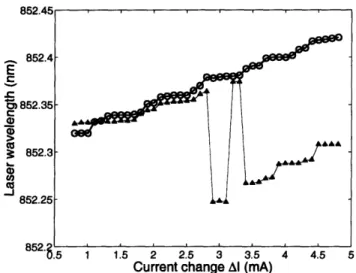
1-1 Atomic levels used in the conditional generation of single photons [2]. 18 2-1 Tuning behavior of laser wavelength with current, for with (open
cir-cles) and without optimal (filled triangles) feedback, measured for an 852 nm laser diode with AR coating. ... 24 2-2 Schematic diagram of the setup used to measure laser frequency noise.
Components like attenuators are not drawn. The polarization of the laser light is out of the plane. ... 24 2-3 Total (open circles) and amplitude (filled triangles) spectral noise
den-sities of an 852 nm AR coated laser assembled with a 1200 mm-l1
grating of reflectivity R1 = 0.21. For frequency noise, 1 V/(Hz)1/2
corresponds to 156 MHz/(Hz)1/2. For amplitude noise, 1 V/(Hz) 1/2 corresponds to a fractional noise of 0.94/(Hz) 1/2 ... 26 2-4 Calculated profiles of 1200 mm- 1and 1800 mm-l1 gratings, overlapped
with diode chip and external cavity modes spaced by frequency inter-vals determined from Fig. 2-1. The width of the passive external cavity mode is calculated for a grating of reflectivity R1 = 0.61 and diode chip
back facet reflectivity[3] : 0.3. The width of the passive diode chip
mode is calculated for an AR coated diode chip with the above back
facet reflectivity and front facet reflectivity[3] 0.003. ... 28 2-5 Plot of linewidth versus current injected into the diode laser. The laser
jumps to a different longitudinal cavity mode near 52 mA. ... 29 9
2-6 Schematic diagram of mount B. The four nylon pull screws that attach
the two aluminum blocks to each other are not drawn. ... 31
2-7 Frequency noise power spectral densities for mount B (open circles) and mount A (filled triangles) lasers. Mount B only has a mechanical resonance at 500 Hz, whereas mount A has mechanical resonances at
2 kHz ... 31
2-8 RMS jitters of lasers assembled both with mount B (open circles for unlocked and solid line for locked) and mount A (filled triangles for unlocked and dashed line for locked). The RMS jitter is given by
Avjitter(f)
-[fol((f))2df']12
p
p.
T we
32
3-1 Atomic levels used in the generation of photon pairs. The write pumpbeam is red-detuned from atomic resonance by 6 = 150 MHz ... 34 3-2 Two-level system of an atom coupled to a cavity. The first label (e,
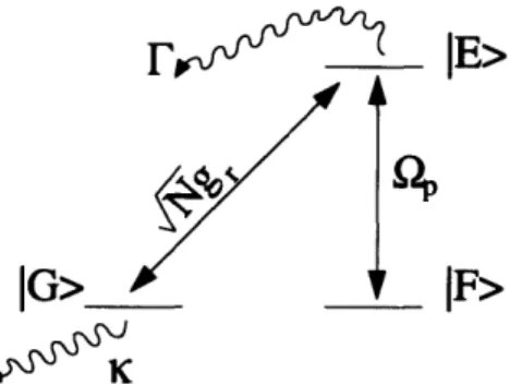
g) denotes whether the atom is in the excited or ground state. The second label denotes the number of photons in the cavity. is the cavity linewidth and r is the natural linewidth of the le) -, g) transition. 35 3-3 Atom-cavity states, couplings and rates of decay involved in the read
process ... 37 3-4 Momenta of write and read laser pumps, which generate the write and
read photons respectively. The write and read laser pumps are aligned to be counter-propagating, whereas the write and read photons are emitted into the cavity mode. The dashed lines depict the spin grating
obtained from interfering the write pump and emitted write photons. 39 3-5 Time-dependent probability for the read photon to be emitted into the
cavity, where t = 0 is the time when a write photon is emitted into the cavity ... 41 3-6 Cavity filtering of the write photon results in good overlap with the
almost-dark state III) for the read process. ... 42
3-7 Time-dependent probability for the read photon to be emitted into the cavity, where t = 0 is the time when a write photon has left the cavity. 43
3-8 (a) Atom-cavity states, couplings, and rates of decay involved in the write process. (b) The two-level system that effectively describes the write process, in the limit of large laser detuning 6. ... 44
4-1 Experimental setup for generating correlated photon pairs. The cavity
lock light is a grating laser beam sent through the cavity in between
sequences of data taking, so as to probe and lock the cavity frequency to atomic resonance. The MOT beams and an additional laser used in optical pumping are not drawn. In the detection setup, "w" and "r"
denote write and read photons, while "v" and "h" denote vertical and
horizontal polarizations respectively. ... 48
4-2 Setup for obtaining the write photon autocorrelation, which is equiv-alent to measuring the cross correlation of the two SPCMs. The read photon output port of the polarizing beam splitter needs to be blocked to prevent reflections back through the cavity and into the write pho-ton output port, which would lead to an artificial increase of the write
photon autocorrelation. . . . ... 50
4-3 Cross and autocorrelations for write and read photons, plotted as a
function of bin width T. gr (green) is combined with g,,,, (red) and
grr (blue) to yield highly non-classical values for the normalized cross correlation G (black) [4] ... 51
4-4 (a) Cross correlation between v-polarized write and h-polarized read photons. A finite cross correlation at negative r simply corresponds
to the detection of read photons before the write photons leave the
cavity. (b) Cross correlation between s-polarized write and f-polarized read photons, also known as the Hong-Ou-Mandel configuration. The dashed green curve and solid red curves are fits to the data, for write and read photon frequency differences of AwI/27r = 0 and Aw/2r =
2.5 MHz respectively [4] ... 52
4-5 Setup for measuring write and read photon cross correlations in the Hong-Ou-Mandel configuration. ... .. 53 5-1 Mach-Zehnder interferometer with two 50/50 non-polarizing beam
split-ters and two mirrors ... 56
5-2 Classical input and output electric fields of a 50/50 non-polarizing beam splitter [1]. ... 57 5-3 Two possible implementations of the Holland-Burnett scheme for nhb =
1: (a) Sending the polarization-separated write and read photon pairs through a spatial Mach-Zehnder interferometer, formed by two 50/50 non-polarizing beam splitters and two mirrors; (b) Sending the write
and read photons through a variable retarder before polarization-separating them ... 58
5-4 Ratio of phase uncertainties, plotted as a function of phase for various fringe visibilities 0. The ratio diverges at 0 = r/2 for all 3 < 1. .... 63 5-5 (a) Voltage output of avalanche photodiode during a scan of the
vari-able retarder voltage. (b) Calibration of phase imparted by the varivari-able retarder versus applied voltage. ... 64 5-6 Hong-Ou-Mandel interference fringes, measured using the variable
re-tarder setup. The red curve is a fit of the data to g,,, = a(l+3 cos('yO+ e))/2, yielding a periodicity of y = 1.93 ± 0.04 and fringe visibility
,3 = 0.84 ± 0.04 ... 65
6-1 "Extraordinary" and "ordinary" photons (i.e. h- and v-polarized
pho-tons) are emitted into two separate cones ke and ko during type-II parametric down conversion. Photons traversing along the points of
intersection between the two cones are entangled [5]. ... 68 6-2 Atomic levels used in generating entangled photon pairs. ... 70 6-3 Cross correlations between write and read photons generated using
the new optical pumping scheme. The photon polarizations have been converted to (a) h and v, or (b) s and f, by the quarter-waveplate. The
flatness of 9hom,,(r) in (b) indicates that the photon pairs are entangled. 71
6-4 Hong-Ou-Mandel interference fringes, obtained by analyzing g,,r(r = 0) in 100 ns bins for different retarder phase shifts. The red curve, which is a fit to the data, has periodicity ?yd = 1.94 ± 0.01 and fringe
visibility 0/ = 0.77 ± 0.03 ... ... 73
6-5 Hong-Ou-Mandel interference fringes, obtained by analyzing (a) gr,,iq(r = -30 ns) and (b) gr,,i(7r = 20 ns) in 20 ns bins. Since neither fringe is symmetric about 0b t 90°, the photons are not maximally entangled. . 74 6-6 Pion decay in an EPR gedankenexperiment. & and b are unit vectors
along which the two detectors may be aligned ... 76 6-7 Setup for proposed implementation of the EPR experiment. ... 77 7-1 Setup for holographic storage of atomic excitations. ... 82
List of Tables
2.1 Linewidths of 852 nm lasers built with different gratings. ... 27
2.2 Linewidths of both AR and non-AR coated 780 nm lasers. ... 29
2.3 Best achieved linewidths of 852 nm and 780 nm lasers. ... 30 A.1 Hong-Ou-Mandel interference fringe fit coefficients, estimated
proba-bility amplitudes, and estimated backgrounds ... 88
Chapter 1
Introduction
The single photon is the most basic ingredient in quantum optics. Single photon states can build up to form number states, or Fock states, which are conceptually simple for physicists to work with: a system described by the number state IN) contains only N photons. How can one obtain a single photon in the first place? One possible way is to excite a single atom, which in turn emits a single photon as it transitions
to the ground state. However, it is not a trivial task to efficiently execute the single
photon emission process in a controlled manner; typically, such a process is subject to Poisson statistics. What is instead desired is a "single photon gun" that can be
"loaded" and "shot" at one's will.
It turns out that a cloud of cesium atoms, weakly coupled to a low-finesse cavity, can act as a conditional single photon source, as realized by the VuletiC group a few months before I joined the experiment [2, 6]. The procedure of "loading the gun" involves sending a highly attenuated "write" laser pulse through the atomic cloud, such that on average one atom is pumped into a different state I1) by the laser (and emits a "write photon" in the process; see Fig. 1-1). It is important that the atoms be
collectively coupled to the cavity, so that the experimentalist is unable to tell which
of the atoms had been excited. As long as any "which-atom" information remains unavailable, the "shooting" of the "single photon bullet" (i.e. the "read photon") can be accomplished with reasonable efficiency at some later time T,,, when a "read"
laser pulse pumps all the atoms back to the original state 10).
(b) 4,ee
I1
Figure 1-1: Atomic levels used in the conditional generation of single photons [2]. One can imagine modifying this idea of a conditional single photon source to obtain a photon pair source, by shortening the delay time T,,r between the application of the write and read laser pulses. In the limit where both the write and read laser beams are applied continuously, one might be able to generate continuous pairs of write and read photons! This is essentially the idea behind our present photon pair source, with some additional modifications to the single photon setup (e.g. using different atomic levels) that we shall not address for now.
Equipped with a source of photon pairs, one can perform a variety of experiments, such as sub-shot noise interferometry [7], tests of the Einstein-Podolsky-Rosen (EPR) paradox [8], and quantum cryptography [9]. One question, however, begs to be asked:
given that correlated photon pairs have been produced since the advent of the
para-metric down converter (a non-linear crystal that outputs a pair of photons with frequencies that add up to the frequency of its input laser beam) in 1970 [10], what advantages do the Vuleti6 source of photon pairs provide over the parametric down converter?
The answer to the above question lies in the bandwidth of the photon pairs pro-duced by the two sources. Pairs propro-duced by parametric down converters tend to have broad frequencies, with widths on the order of 100 GHz [10]. Novel quantum communication schemes, however, require photon bandwidths on the order of 1 MHz
18
[11], which - surprise, surprise - the Vuletic source is able to provide!
Some of the most dramatic capabilities of our photon pair source are summarized
in a paper submitted for publication [4]. One aim of this thesis is to provide
in-tuitive pictures explaining the physics behind the generation of narrowband photon pairs in our setup. Chapter 3 gets to the heart of the physics by modeling the cloud
of cesium atoms in a cavity as a three-level system. The experimental
implementa-tion and evidence for the correlated photon pairs are then described in Chapter 4.
Two applications of the new photon pair source, which form the actual focus of my thesis work, are presented in Chapters 5 and 6. Chapter 5 describes a two-photon
interference experiment that offers the potential to achieve sub-shot noise precision,
while Chapter 6 shows how the collectively coupled atoms can serve as a resource for polarization-time entangled photons. Finally, Chapter 7 concludes with a summary
and outlook of the atom-cavity system.
What about Chapter 2? In Chapter 2, we take a step back from all the excitement
about photon pairs, and examine instead an important tool employed in almost every
atomic physics experiment, including this one: the grating-tuned diode laser. Specifi-cally, Chapter 2 describes the work I carried out to determine the influence of grating parameters on the linewidths of external-cavity diode lasers. For completeness, I have also included some linewidth measurements by Yu-Ju Lin and Marko Cetina, and Igor Teper's design of a diode laser mount with improved mechanical stability [12].
Chapter 2
Linewidths of Grating-Tuned
Diode Lasers
2.1 Motivation and Background
Diode lasers have vast applications in atomic physics, because of their reliability, easy tunability, and low cost [13, 14]. Diode lasers alone, however, have linewidths of around 20 MHz [15], which are often too broad for manipulating atoms, and are typically not tunable to every wavelength of interest. Optical feedback, achieved by adding an external cavity element such as a diffraction grating, not only enhances the wavelength tunability, but also reduces the intrinsic linewidth to below 1 MHz
[13]-[15].
Intrinsic linewidths of several hundred kHz are usually sufficiently narrow for most atomic physics experiments, since strong atomic transitions have typical linewidths of several MHz. However, certain experiments, such as cavity QED experiments [16], or those using narrow atomic transitions [17], require smaller laser linewidth. While it is possible to reduce the linewidth by actively stabilizing the laser to a high-finesse cavity with a fast servo loop [18], it is advantageous to prestabilize the laser by mechanical and optical design. From this practical viewpoint, we are interested in how various
optical components in the grating laser setup - namely the grating, collimator and
diode chip -- affect the intrinsic laser linewidth. We have experimentally investigated
the linewidths of grating lasers in both the near IR (780 nm for Rb, 852 nm for Cs) and near UV (399 nm for Yb) regimes.
The linewidths of lasers have been extensively studied both theoretically [19]-[25] and experimentally [26]-[31]. Theoretical analysis of external cavity diode lasers shows that linewidths narrow with higher optical feedback. Most theoretical papers, however, model the external cavity element as a mirror without any frequency se-lectivity, instead of as a diffraction grating. Considering competition between diode chip modes as a mechanism for linewidth broadening [32, 33], we hypothesize that the linewidth should also depend on how well neighboring chip modes can be suppressed
by the grating spectral profile, as characterized by the grating resolution. The latter is given by A/AA = mNg = m(2D)/[(2/ng) 2- (Am)2]1 /2, where m is the
diffrac-tion order, Ng is the number of illuminated grating lines, D is the beam diameter,
A is the wavelength, and ng is the grating groove density. To our best knowledge, no study has so far been conducted to determine the effect of grating resolution on the linewidth. Furthermore, the influence of an antireflection (AR) coating on the front facet of the laser diode on the linewidth has not been as well studied as its effect on wavelength tunability. Wyatt has reported a significant effect of the AR coating on the linewidth of a 1.5 ptm laser [28], while another experiment showed no effect for a 1.3 m InGaAsP laser [29]. In the present work, we investigate how the linewidths of 780 nm and 852 nm grating-tuned diode lasers are influenced by the grating reflectivity, grating resolution and diode AR coating.
The conventional method for determining the linewidth is to superimpose two laser beams on a sufficiently fast photodiode, which yields the convolution of the spectral profiles of the two lasers. This method relies on the availability of a very narrow reference laser, so that the beat note frequency width mainly reflects the test laser linewidth. In addition, the intrinsic linewidth may sometimes be shrouded by low frequency mechanical vibrations, which may result in a broadened beat note. In
this study, we have instead obtained the linewidth by measuring the power spectral density of the test laser's frequency noise fluctuations, S(f). S(f) is expected to
display higher noise at low Fourier frequencies due to mechanical vibrations. The
noise then falls until it reaches a white noise level, So, at high Fourier frequencies [34]. So is related to the intrinsic Lorentzian linewidth Av by [35]
Av = 7rSO2. (2.1)
To convert frequency noise into intensity noise that can be measured with a photo-diode, either the transmission signal from a Fabry-Perot cavity [36, 37] or the atomic resonance line [34] can be used. The atomic line offers the advantage of being in-sensitive to mechanical vibrations. Using the atomic line to measure noise at low Fourier frequencies, we characterized an improved laser mount, a schematic of which is presented in the final section of this paper.
2.2 Frequency Noise Measurements
A typical grating laser used in this study is assembled in a Littrow configuration [14]. For each assembled laser, we carefully optimize its collimation and grating alignment to achieve the best possible optical feedback using the following procedure: monitoring the laser optical power, we set the laser diode current to just below its threshold value. The current is then dithered with a triangle wave of 100 Hz, and the onset of lasing manifests as a sudden increase in optical power with current. The goal is to minimize the laser threshold by adjusting the collimator position and the grating angle, assuming that the feedback is optimized when the threshold is minimized. The feedback is much more sensitive to the collimator position than to
grating angle [3, 34].
Fig. 2-1 shows how the wavelength of an AR coated laser tunes with current for both optimized and unoptimized feedback. When the feedback is optimized, the wavelength tunes smoothly, with small jumps of 4.5 GHz between external cavity modes. On the other hand, when the vertical grating angle or the collimator lens is slightly misaligned, large frequency jumps of about 50 GHz appear, corresponding to lasing on different residual diode chip modes that have not been completely suppressed
due to imperfect AR coating. 852.4 E m5 852.35 () 3 852.3 )852.25 852.25 I 4 r 3 Q Q0 A A I
Figure 2-1: Tuning behavior of laser wavelength with current, and without optimal (filled triangles) feedback, measured for with AR coating.
for with (open circles) an 852 nm laser diode
Figure 2-2: Schematic diagram of the setup used to measure laser frequency Components like attenuators are not drawn. The polarization of the laser light of the plane.
noise. is out
Once the feedback is optimized, the laser light is sent through an atomic cell and onto an avalanche photodiode with a bandwidth of 300 kHz. The photodiode band-width is sufficient to measure the intrinsic lineband-width, because the white frequency noise typically appears from Fourier frequencies of 20 kHz onwards. Fig. 2-2 shows a schematic of the setup used to measure the laser frequency noise. The laser wave-length is tuned to a value that matches the slope of a Doppler absorption profile (e.g. 852.334 nm for Cs), which allows us to use the atomic absorption line to con-vert the laser frequency noise into amplitude noise for detection by the avalanche
CI.iu r .i a. - .il m)
Current change AI (mA) -fW I I & I I I I I ULr~
our-lo)
photodiode. For the 399 nm laser, the Dichroic Atomic Vapor Laser Lock (DAVLL) dispersive signal [38] from a hollow cathode lamp (Hamamatsu L2783-70HE-Yb) is used instead.
The slope of the absorption line is calibrated by beating the grating laser against a reference laser locked to another atomic cell. The slopes on the two sides of the absorption line are observed to be asymmetric, because of the linear increase in laser output power with wavelength. To remove this linear dependence, we average over measurements on both slopes of the atomic line.
The noise as measured by the avalanche photodiode in Fig. 2-2 contains both frequency noise and amplitude noise, which may or may not be correlated to each other. To measure the amplitude noise alone, we remove the atomic cell and insert gray filters to attenuate the beam power to its previous value on the photodiode. We find that the amplitude noise scales approximately as the square root of the power incident on the photodiode, an indication that the amplitude noise at the frequencies of interest is dominated by photon shot noise, and is thus uncorrelated with the frequency noise. Fig. 2-3 shows both the total noise and the amplitude noise contributions for a typical measurement. The frequency noise is obtained by subtracting the amplitude noise from the total noise in quadrature. The noise below 5 kHz generally reflects the mechanical vibrations of the laser mount, whereas the noise above 5 kHz becomes approximately independent of frequency, indicating a
Lorentzian lineshape [35].
Applying Eq. (2.1) to the white noise portion, we measure typical linewidths of the 780 nm and 852 nm grating lasers to be in the 250-600 kHz range (see Tables 2.1 and 2.2). In fact, we also determine a similar linewidth of 250 kHz for a 399 nm Nichia NDHV310APC laser diode (non-AR coated) assembled with a 2400 mm- 1 grating of reflectivity R1 = 0.60.
For comparison, the method of converting frequency into amplitude noise via the atomic absorption line has allowed us to measure a linewidth as narrow as 30 kHz for a distributed Bragg reflector (DBR) laser diode, whose intrinsic linewidth was narrowed by optical feedback from a low-finesse optical cavity using a setup similar
N
I
v 0 0 Be C 0 0 Frequency (kHz)Figure 2-3: Total (open circles) and amplitude (filled triangles) spectral noise densities of an 852 nm AR coated laser assembled with a 1200 mm-l grating of reflectivity
R1 = 0.21. For frequency noise, 1 V/(Hz)1/2 corresponds to 156 MHz/(Hz)'/2. For
amplitude noise, 1 V/(Hz)l/2 corresponds to a fractional noise of 0.94/(Hz)/ 2. to Dahmani[18] et. al.'s.
2.3 Effects of Grating Parameters and AR Coating
on the Laser Linewidth
Table 2.1 shows the linewidths for various gratings (Edmund Optics 43222, 43753 and 43773) assembled with the same AR coated laser diode chip (Sacher Lasertech-nik SAL-850-50-SDL) and collimator (Thorlabs C390TM-B, effective focal length =
2.75 mm).
As expected from theory, the higher the grating reflectivity R1, the narrower the
linewidth. We also note, from comparing the first and third rows of Table 2.1, that the linewidth narrows with higher grating resolution despite a lower grating reflectivity. Fig. 2-4 gives a physical picture accounting for both effects of grating reflectivity and resolution. The external cavity, formed between the back facet of the laser diode chip and the reflective grating surface, is modeled as a passive Fabry-Perot cavity, whose finesse is first maximized during the feedback optimization procedure described above. Its highest achievable finesse, however, is limited by the reflectivity of the grating
Table 2.1: Linewidths of 852 nm lasers built with different gratings.
Grating part number R1 Ro ng (mm-l) A/AA Av (kHz)
43773 0.21 0.67 1200 4200 560 ± 140 43753 0.61 0.19 1200 4200 440 110 43222 0.16 0.78 1800 8400 320 + 60
Linewidths of AR coated 852 nm lasers built with gratings (from Edmund Optics) of different reflectivities into the first and zeroth diffraction orders R1 and Ro respectively, and different groove densities ng. For a Littrow grating laser, the first diffraction order is reflected back into the laser for optical feedback, while the zeroth order is used as the laser output. R1 and
Ro are measured values, while the grating resolution A/AA is computed for a beam diameter of D _ 3 mm.
chosen. The grating resolution, on the other hand, sets the width of the grating profile in Fig. 2-4. A higher grating resolution, achieved with a grating of higher groove density or a collimator that produces larger beam size, better suppresses neighboring diode chip modes, leading to less mode competition and hence less frequency noise. In fact, the greater influence of the grating resolution on the linewidth reduction indicates that the suppression of other laser diode chip modes is more important than the finesse of the external cavity.
The results in Table 2.1 imply that one may be able to obtain a narrower linewidth by simply using a grating of higher groove density, while keeping the zeroth order reflectivity Ro and laser output power high. In addition, we attempted to increase the grating resolution by using a collimator that produced a larger beam size (Thorlabs C240TM-B, effective focal length = 8.0 mm). We found that even when the optical feedback was only near-optimized, we could already achieve a linewidth of 425 kHz using the 1800 mm-l1 grating. On the other hand, the combination of the larger beam size and 1800 mm-l1 grating also means that the optical feedback is much more sensitive to the grating angle. At such high sensitivity, slight thermal drifts of the aluminum laser mount made it extremely difficult for the grating to remain at its optimal angle. As a result, we were unable to maintain reliable operation in the mechanical setup of Fig. 2-2 for this collimator-grating combination.
9
.E >1 C C 2 Frequency (GHz)Figure 2-4: Calculated profiles of 1200 mm- 1 and 1800 mm- 1 gratings, overlapped with diode chip and external cavity modes spaced by frequency intervals determined from Fig. 2-1. The width of the passive external cavity mode is calculated for a grating of reflectivity R1 = 0.61 and diode chip back facet reflectivity[3] - 0.3. The
width of the passive diode chip mode is calculated for an AR coated diode chip with the above back facet reflectivity and front facet reflectivity[3] . 0.003.
We also study the effect of an AR coating on the linewidth. Table 2.2 shows the linewidths of AR coated and uncoated laser diodes assembled with the same grating
(R1 = 0.27, n = 1200 mm-1). Although the AR coated laser has a slightly narrower
linewidth, the estimated error bar associated with each measurement is approximately 100 kHz. We hence conclude that although the AR coating eases the procedure for optimizing grating alignment as well as enhances wavelength tunability (Fig. 2-1), its effect on the linewidth is insignificant.
Table 2.2: Linewidths of both AR and non-AR coated 780 nm lasers.
Diode Model AR Coating Av (kHz)
Sanyo DL7140-201 No 500 + 100 SAL-780-40 Yes 450 ± 100
Linewidths of 780 nm lasers with and without an AR coating on the front facet. A grating (Edmund Optics 43773; see Table 2.1) is used.
of current injected into the diode laser influences the extent to which the laser op-erates in a single mode, which in turn affects the linewidth (Fig. 2-5). When the laser is about to jump to a different mode, it becomes slightly multi-mode and the linewidth increases by an order of magnitude due to mode competition. Although we have verified that the laser operated in a single mode during our frequency noise measurements, Fig. 2-5 shows that there is still a linewidth variation of about 80 kHz in the single-mode regime.
I
-c_
.. J
Current (mA)
Figure 2-5: Plot of linewidth versus current injected into the diode laser. The laser jumps to a different longitudinal cavity mode near 52 mA.
Table 2.3 summarizes the smallest linewidths obtained for the near IR diode lasers (780 nm, 852 nm). For comparison, the linewidth of the near UV laser (399 nm) is included.
Table 2.3: Best achieved linewidths of 852 nm and 780 nm lasers.
Atoms A (nm) AR Coating R1 ng (mm-') A/AA Av (kHz)
Cs 852 Yes 0.16 1800 8400 320 ± 60 Rb 780 Yes 0.27 1200 4100 450 i 100 Yb 399 No 0.60 2400 8200 250 - 70
Smallest achieved linewidths of 852 nm and 780 nm lasers and their cor-responding diode and grating parameters. For comparison, the linewidth of the 399 nm laser is listed.
2.4 Mechanical Stability of Laser Mounts
Fig. 2-6 shows a new laser mount ("mount B") that is designed to reduce mechanical oscillations at higher acoustic frequencies. For the regular mount[14] ("mount A"; see Fig. 2-2), the grating and laser diode are separately attached to a third aluminum piece that serves as the base of the mount. The vertical and horizontal grating angles are adjusted by turning the screws of the mirror mount. Conversely, for mount B, the aluminum block containing the grating is attached directly to the block containing the laser diode via four nylon pull screws. Three stainless steel screws, which push on a rubber ring and a piezo stack sandwiched between the two blocks, respectively, allow the vertical and horizontal grating angles to be adjusted with better resolution. In fact, the vertical angle only needs to be adjusted slightly, because the optical feedback is already near-optimal when the grating sits flush in the machined pocket. Mount B also includes a mirror, which couples the beam out of the mount in a fixed direction regardless of the grating's horizontal angle [39].
Plexiglass cover .. _._._._._._._._.. ... Piezo stack -Rubber ring i ! beam -path t Rubber ! ring i i Mirror I
Screw for horizontal Laser Diode Screws for vertical
grating alignment grating alignment
Figure 2-6: Schematic diagram of mount B. The four nylon pull screws that attach the two aluminum blocks to each other are not drawn.
The mechanical properties of mount B are characterized in terms of its frequency noise power spectral density and root-mean-square (RMS) jitter at low Fourier fre-quencies (up to 5 kHz), and are plotted in Fig. 2-7 and 2-8 respectively. For compar-ison, Fig. 2-7 and 2-8 also display the data for a laser assembled with mount A. At first glance, mount A appears to be more stable than mount B, because its overall noise is lower. However, the low frequency noise can often be easily reduced with a
i
feedback circuit. In fact, the lower the frequencies at which resonances occur, the easier it is for the feedback circuit to compensate for noise. In this respect, mount
B is better than mount A, because its mechanical resonance only occurs at 500 Hz,
whereas mount A has resonances at around 2 kHz. As shown in Fig. 2-8, the RMS jitter of the laser built with mount B is much lower than that for mount A, when both lasers are locked. Integrating from 0 Hz up to a bandwidth of f = 10 kHz, we achieve RMS jitters of AVjitter(f) = [of(S(f'))2df']1/2 = 40 kHz and 100 kHz for the actively stabilized lasers built with mounts B and A, respectively.
4 5 N I a) .) z .0 Z a) 0 a) U-10' 10o 10 10' Frequency (Hz)
Figure 2-7: Frequency noise power spectral densities for mount B (open circles) and mount A (filled triangles) lasers. Mount B only has a mechanical resonance at 500 Hz, whereas mount A has mechanical resonances at 2 kHz.
2.5 Summary of Linewidth Studies
We have measured frequency noise power spectral densities to determine laser linewidths for various grating laser setups. We find typical linewidths of 250-600 kHz for lasers operating near 399 nm, 780 nm and 852 nm. The linewidth depends on the type of grating and collimator. The presence of an AR coating has an insignificant effect on the linewidth reduction, but enhances tuning stability. On the other hand, the higher the grating reflectivity and grating resolution, the narrower the linewidth. In particular, the grating resolution has a larger effect on the linewidth than the grating
DUU 450 400 N I 350 300 .5 250 C) 2 200 150 100 50 n =- …= 01 102 103 104 Integration Bandwidth f (Hz)
Figure 2-8: RMS jitters of lasers assembled both with mount B (open circles for unlocked and solid line for locked) and mount A (filled triangles for unlocked and dashed line for locked). The RMS jitter is given by Avjitter(f) = [ofS(f))2dfl]]1/2
reflectivity.
Using a new laser mount with improved mechanical properties, we were able to achieve an RMS jitter of 40 kHz for an actively stabilized system with a loop band-width of only 1.5 kHz.
550. 1, - . ,-·-- ·- ·, - ·-
Chapter 3
Cesium Atoms in a Cavity: a
Three-Level System
3.1 Atomic Transitions Used in Cesium
Chapter 1 has already provided a brief introduction to the idea behind generating pairs of write and read photons. Fig. 3-1 shows the relevant cesium energy levels that the r-polarized write and read laser pumps interrogate to produce the cor-responding write (+-polarized) and read (a--polarized) photon pairs. For conve-nience, we denote the atomic states as the following: a) - IF = 3, mF = -3),
lb)-IF' = 3, m' =-3),
If)
-IF = 3, mF =-2), e)
IF'
= 2, m' =-2), where F, F'
are quantum numbers that label the ground state 62S1/
2 and excited state 62P3/2
re-spectively. Because all the atoms are optically pumped to a) initially, the read process
(If)
-- le) -+ la)) can only take place after the write process transfers an atom from la) toIf).
The write process, however, can "reverse" itself as the interrogated atom Rabi-flops from If) back to la) via b). To reduce competition between the read and reverse-write processes, we use a far-detuned write laser pump and an on-resonance read laser pump. Since the spontaneous emission rate goes as the inverse-square of the laser detuning 6 for large [40], the read process occurs much more quickly than the reverse-write process.mF: -3 -2 6p 2 F'=3 lb)
63/2 F' =2e)
6
2S,,
F =3
I w: write photon r: read photon Ia) If)Figure 3-1: Atomic levels used in the generation of photon pairs. The write pump beam is red-detuned from atomic resonance by 6 = 150 MHz.
of how the read photon can be generated conditionally on the write photon. However, the ability to generate photon pairs does not necessarily translate into the ability of detecting photon pairs! The issue is that an excited atom emits a photon into 47r steradians when it makes a transition back to the ground state. Unless we had a special device that could collect the photons emitted into all possible solid angles, we would have a very low detection efficiency, limited by Afet/ 4 7, where AQde,t is the solid angle subtended by the detector.
The low-finesse, single-mode cavity that the cloud of cesium atoms are weakly coupled to provides an alternative solution to the special detecting device. Instead of collecting photons emitted into 4r steradians, the cavity enhances the emission of photons into its single cavity mode [41]. The photons then leak out of the cavity at a rate given by the cavity linewidth n into a detector outside of the cavity. To develop a common language describing the coupling of the cesium atoms to the cavity, the concept of a single atom's cooperativity r7 to the cavity mode will now be introduced.
3.2 Cooperativity Parameter
The cooperativity parameter describes how well a single atom can emit a photon into one direction of a single cavity mode compared to that into free space. From geometrical considerations, goes as the ratio of the solid angle subtended by the
cavity mirror A\Qc to 47r, and is enhanced by the cavity finesse F. AQc/47r in turn
goes as (A/Wc)2, which can be thought of as the number of photons of wavelength A that can "fit" into an area characterized by the cavity mode waist wC. Putting in all the numerical factors, we get [41, 42]:
2r
3 ()
(3.1)
Fig. 3-2 offers a different perspective on the cooperativity parameter. The levels depicted in Fig. 3-2 correspond to an atom in the excited state (in our case, 62P3/2)
with no photons in the cavity le, 0), and an atom in the ground state (62S
1/2) with one
photon in the cavity g, 1). The two levels are coupled by a Rabi frequency g, which is the single-atom vacuum Rabi frequency as extracted from the Jaynes-Cummings model [43]. For an atom initialized in le, 0), q is given by the probability of emitting
a -photon into the cavity mode compared to that of emitting a F-photon into free
space:
g2// g2
7/= K (3.2)
Ig,l> le,O>
K
F'r
Figure 3-2: Two-level system of an atom coupled to a cavity. The first label (e, g) denotes whether the atom is in the excited or ground state. The second label denotes
the number of photons in the cavity. K is the cavity linewidth and r is the natural
linewidth of the le) -, g) transition.
Both expressions for turn out to be equivalent, although Eq. (3.2) is more convenient for explaining the physics in the following sections. Ideally, we would like
7 to be as large as possible, so as to achieve a high directionality in the emission of
the write or read photon. On the other hand, it is technically challenging to strongly
couple a single atom to a high-finesse cavity with a small mode waist. The way we
circumvent this problem is to collectively couple N, atoms to a cavity. As long as
Natl > 1, a photon will be emitted into the cavity mode with a high likelihood, even
for the case of a low-finesse cavity.
3.3 Superradiance on the Read Process
For the write process, achieving Narl > 1 is trivial: the factor Na comes from the fact that there are initially Na atoms in the ground state, all of which can be possibly excited. Meeting the same condition Nat7 > 1, however, is not as intuitive for the read process. Afterall, when the read process is initialized, only one atom will be in
If) (see Fig. 3-1)! How then does the read photon get preferentially emitted into the cavity mode?
The trick is that the write process must drive an atom from la) to If) in a way that
the experimentalist is unable to tell which atom had made the transition. Eq. (3.3)
show the states used in the read process, including now an additional label for the number of read photons in the cavity Inr) (see also Fig. 3-3). Because the atom that is driven to If) cannot be identified, one must symmetrize the states of the read process
[44, 45]:
1 Na 1 Na
IF) - Ifi aj) r)-- i) r) (3.3a)
i--1
ji
7/a
i--Na 1N
IE) -- lei aj) 1 E lei) 1, (3.3b)
i=l ji a i=l
Na
IG) -- | la i) r )--l a ) (3.3c)
i=l
Since the j Z i atoms are always sitting in la), the labels laj) are dropped for convenience.
The on-resonance Rabi frequencies that couple the symmetrized read states are
ran~1_
IE>
IG> IF>
Figure 3-3: Atom-cavity states, couplings and rates of decay involved in the read process.
then given by the following expressions:
Q2FE = Qp, (3.4a)
QEG = V/-gr, (3.4b)
where QP is the Rabi frequency of the read pump beam interacting with one atom. The expression for Q2FE comes as no surprise, for only one atom is making the atomic
transition If) - le). The scaling of QEG with the square root of the number of atoms,
however, is unexpected. The following equation provides a more careful computation
of QEG:
QEG -(G
E
E)
= (G
gr(&+a
+
&at_)IE)
Na
g {(al (lrI} (+a + at&-) {Ie,) 1or)}
r N(3.5)
-/agr. (3.5)
The first and second lines in the above equation rewrite the usual Hamiltonian for a
two-level atom interacting with an electric field -d. E in terms of the read photon creation at and annihilation operators, and operators describing the la) +-, le) atomic transitions i.e. + = le)(al and &_ = la)(el [43]. Simply put, the term &+a
takes an atom from la) and puts it in e) while absorbing a read photon from the
cavity mode, and vice versa for &ta_. The last few lines of the calculation tell us that
the VN factor comes from coupling a symmetrized state to a product state upon
the emission of a read photon. Returning to Fig. 3-2 with QEG = /JNgr instead of
merely gr, we find the cooperativity for the emission of the read photon to be
(V r)2 K = Na r = Narl. (3.6)
IK
Eq. (3.6) shows that the read photon is Na times more likely to be emitted into the cavity mode than expected for a single atom in the excited state. Such collective enhancement of spontaneous emission is also known as Dicke superradiance [44].
3.4
Four-Wave Mixing
Up to this point, we have ignored in our discussion of superradiance the finite spatial extent of the atomic cloud. Since the cloud of atoms is larger than the wavelength
of the emitted photons, a spatial phase-matching condition must also be fulfilled to
achieve superradiance [44]:
Pr,photon = P,pump - Pw,photon + Pr pump (3.7)
Fig. 3-4 illustrates the phase-matching condition, where P is the momentum of the
photon indicated in the subscript. In our case, the phase-matching condition is
sat-isfied by retro-reflecting the write pump beam to produce the read pump beam. Since the momenta sum to zero, and the initial and final states of the system
remain the same (i.e. all atoms in a)), the generation of the write and read photon pair can be viewed as a four-wave mixing process. In the language of four-wave mixing, we now have another picture for the superradiant emission of the read photon: the incoming write pump beam and the outgoing write photons interfere to form a spin grating in the atomic cloud (depicted by the dashed lines in Fig. 3-4). The incoming
read pump beam then scatters off the atomic grating to give outgoing read photons.
P
r,pump
#-
-Ip t w,pump
Pw,photon
Figure 3-4: Momenta of write and read laser pumps, which generate the write and
read photons respectively. The write and read laser pumps are aligned to be
counter-propagating, whereas the write and read photons are emitted into the cavity mode. The dashed lines depict the spin grating obtained from interfering the write pump and emitted write photons.
Because it is Na times as likely for a write photon to be scattered into the cavity mode, the emission of the read photon into the cavity is also enhanced by Na. (The emission
of the write and read photons into opposite directions does not matter, because both photons will circulate within the cavity anyway.)
3.5 Three-Level System Dynamics on the Read
Process
Superradiance, while a rich phenomenon itself, does not give the full physics associ-ated with the read process. Instead of focusing on the coupling between states E) and G), we return to the full three-level system depicted in Fig. 3-3.
The reader is reminded that the couplings QFE and f2EG occur on atomic reso-nance. For the moment, we shall ignore the fact that photons can decay out of the
system via r, and F. Using the interaction picture in the {IF), E), IG)} basis, the
three-level system can then be described by the Hamiltonian
H = [2P (IF)(El + E)(FI) + g (G)(EI + E)(G)] , (3.8)
with eigenvalues and eigenstates
E = hQ' : II) = (P F) + -galr IE)+ / IG)),
Eli = -hQ': III) = (P IF) - ' IE) + Ng,. G)), (3.9)
EIII= 0 : IIII)= (V-,(gr F)
-PG)),where Q' = [(2Qp/2)2 + Nag2]/ 2. Note that the third eigenstate is special: it has
no excited state component. In conventional three-level physics terminology, 1111) is also known as the dark state, because it cannot spontaneously emit any photons by making a transition from IE) to any of the two ground states [43].
We now allow the read photon to leave via nc and r decay, as the system transitions back to a fourth level IA)
HIJ
ljai) 10,). The master equation approach gives the most general description of the system [43, 46]:1
1= [H, p] + rA)(EI p IE)(AI + K IA)(GI p IG)(AI
ih
-2 (IE)(E p + p E)(EI) - (IG)(GI p + p IG)(GI) , (3.10)
where H is the Hamiltonian from Eq. (3.8) and p is the density matrix of the
four-level system. It turns out that, because the ic and r photons decay out of the
three-level system, the four-three-level master equation approach is equivalent to the Schr6dinger wavefunction approach for a modified three-level interaction Hamiltonian:
ihn = H',O, H' = H- i( IE)(EI + 2 IG)(GI), (3.11)
where 0b is the wavefunction of the system.
Under the modified Hamiltonian, the states IE) and IG) have some imaginary width corresponding to their decay rates. In the basis of eigenstates, has no effect
on the dark state, although it pulls the other two eigenenergies EJ and EII closer to
each other [47]. On the other hand, K "spoils" the dark state by coupling some excited
state component into 111I). Returning to our original goal of photon pair generation, we see that we would like as many photons to leave from IG) as possible, instead of
losing them via r-decay from E). Therefore, to achieve a high recovery efficiency of
the read photon, we need to be well-overlapped with the "almost-dark" state
EIII),
which is also the state with the least (albeit finite) excited state component.
We expect the read photons to be emitted with an exponential decay in time (where initial time is defined to be that when a write photon is emitted into the
cavity) if the overlap with the almost-dark state is perfect. Otherwise, the admixture
of other eigenstates shows up as Rabi-flops in the time-dependent emission of the read photons, as simulated in Fig. 3-5.
4 t (s)
Figure 3-5: Time-dependent probability for the read photon to be emitted into the cavity, where t = 0 is the time when a write photon is emitted into the cavity.
When a write photon is emitted into the cavity, the system is initialized in a superposition of all three read eigenstates. How then can the system have a strong overlap with the almost-dark state? In our experiment, the frequency of the single
cavity mode has been tuned to coincide with atomic resonance. Because EIm 0,
the write cavity mode is nearly resonant with the almost-dark state, while the other eigenenergies E and EJ, are filtered out by the frequency width of the write cavity
(see Fig. 3-6). Hence, as the write photon leaks out of the cavity and into the detector, the phases of the two "bright" eigenstates II), II) cancel out, and what remains is a
coherent overlap with the almost-dark state 111).
In the time domain, the cavity filtering of the write photons is equivalent to con-volving the amplitude of read photon emission (Gl,0(t)) with the amplitude of write
Write Eigenenergies of
cavity Read Process Hamiltonian
mode E
El,,
Figure 3-6: Cavity filtering of the write photon results in good overlap with the
almost-dark state IIII) for the read process.
photons decaying out of the cavity e-( /2)t. It is important that the convolved
quanti-ties be amplitudes instead of probabiliquanti-ties, for the following reason: both (G[I(t)) and
e- ( /2)t have t = 0 defined as the time when a write photon is emitted into the cavity.
However, there is no way of finding out when a write photon is actually emitted into the cavity without making a measurement that disturbs the system dynamics. Our
knowledge of when the read photon is emitted is smeared out by the time over which the write photon leaves the cavity for the detector, therefore one can only add ampli-tudes instead of probabilities. In other words, the above convolution of ampliampli-tudes is analogous to the Feynman path integral [48], where the "paths" in this case are
indistinguishable time paths for the write photon to be emitted. Fig. 3-7 shows the
result of convolving Fig. 3-5 with e-( /2)t, which is the time dependent probability of
emitting a read photon into the cavity, where initial time is now defined to be that
when a write photon has left the cavity.
3.6 Write Process
We examine the mechanism responsible for initializing the read process: the write process. Like in the read process, there are three states involved in the write process
0 0-o. e c Cu 0 Uo E
a
5 (s)Figure 3-7: Time-dependent probability for the read photon to be emitted into the
cavity, where t = 0 is the time when a write photon has left the cavity.
(see Fig. 3-8a):
Na
IA)
Hai) 10),
II
(3.12a)
i=l Na 1
IB)
=n
Ibi
a)
10) ,
(3.12b)
i=1 ji Na IC) a (3.12c) i=1 jiThe Rabi frequencies coupling the states are QAB = /N-awp and QBC = g,, where wp is the Rabi frequency of the write pump beam interacting with one atom.
One key difference between the two processes is the fact that all Na atoms start
in the la) state, which is to be contrasted with only one atom starting in the If) state for the read process. Another major distinction is that the write laser is red-detuned
by 6 = 150 MHz from atomic resonance. The large detuning (6 > AB, Q2BC) allows us to simplify the three-level system into a two-level one, where the two levels IA) and IC) are coupled by an effective two-photon Rabi frequency (see Fig. 3-8b):
e.ff = V aJWpg. (3.13)
43
r
Fed IRS.
(h)
e
4-.' nQeff
I- I
It> -IA>
Figure 3-8: (a) Atom-cavity states, couplings, and rates of decay involved in the write process. (b) The two-level system that effectively describes the write process, in the limit of large laser detuning .
The write photon then leaks out from C) via n decay. Note that r does not enter the
description of the effective two-level system, because the system is merely reinitialized in A) when the excited atom decays back to its ground state a).
Since (Qeff << I at large detuning, the write process operates in the rate equation
limit. In other words, there is no Rabi flopping between IA) and C), and write
photons simply get injected into the cavity at the constant rate [42]
RAC = eff 1((3.14)
In fact, there is an even simpler picture describing the rate at which write photons are emitted into the cavity. For small Qeff, the problem of spontaneous emission
reduces to an off-resonant scattering problem. The rate at which write photons are
scattered off the write pump beam into free space, in the limit of large 6, is given by
[40]:
Rf (2-) ' (3.15)
where I and I are the applied and saturation intensities respectively. The rate at
which write photons are scattered into the cavity is then enhanced by the collective
cooperativity Nar:
Ra = NrRf =_ (
Rcav~~an rs-2r2agI
432) \2 I8)(3.16)
44
X-I . I "%
-Using the relation
2(wp/r)
2 = I/I8, we reconcile the two pictures describing the emission of the write photon: R,, = RAC.3.7 Summary of Write and Read Processes
Many important ideas have been presented in this chapter - cooperativity,
superra-diance, four-wave mixing, and the three-level system in both the strong coupling and
rate equation limits. We reiterate how these concepts fit together in the mechanism
for generating correlated photon pairs: initially, all the atoms are optically pumped
to a). One of the collectively coupled atoms off-resonantly scatters a write photon from the write laser beam as it makes a transition from la) to If) at a constant rate
RAC. Given this constant rate, the emission of the write photon into the cavity
ini-tializes two processes: the exponential decay of the write photon out of the cavity, and the read process. For the read process, the emission of the read photon into the cavity mode is enhanced by superradiance (or four-wave mixing, which is equivalent to superradiance in an extended sample), because we are unable to tell which of the
atoms had made the la) - If) transition. The time-dependent probability amplitude
for the read photon to be emitted is governed by three-level dynamics, which must be convolved with the exponentially decaying time dependence describing when the emitted write photon leaves the cavity. Such a convolution encodes a strong overlap
between the state of the system and the almost-dark state (i.e. very little excited
state e) component) for the read process. Good overlap with the almost-dark state
ensures that most of the read photons decay into the cavity mode instead of into free
space, which translates into high recovery efficiency of the read photons.
Chapter 4
Generation of Correlated Photon
Pairs
4.1 Experimental Setup
Modeling the cavity and collectively coupled cesium atoms as a three-level system has provided us with an understanding of how correlated write and read photon pairs can be generated. We now turn to the practical details of the experiment. This section gives a sketch of the key components of the experimental setup used to generate correlated photon pairs. Technical details of the laser system, optical pumping procedure and magneto-optical trap (MOT) holding the cesium atoms can be found in Adam Black's thesis [6].
Fig. 4-1 shows a schematic diagram of the experimental setup. The cesium atoms are held by a MOT in a low-finesse ( = 250), single-mode cavity, of which N 104
atoms are positioned at the waist (w, = 110 im) of the TEMoo cavity mode. The Rabi splitting due to a single atom coupled to the cavity is given by 2g/27r = 0.36 MHz, and the single atom cooperativity is r7 = 7.3 x 10- 4, which translates to a collective cooperativity of Nar7 5. 7r-polarized, counter-propagating write and read laser pump beams are applied continuously from the side of the cavity. The read pump beam is derived by retro-reflecting the write pump beam off a mirror, hence
![Figure 1-1: Atomic levels used in the conditional generation of single photons [2].](https://thumb-eu.123doks.com/thumbv2/123doknet/14050256.460088/18.918.285.575.111.370/figure-atomic-levels-used-conditional-generation-single-photons.webp)