HAL Id: tel-00859843
https://tel.archives-ouvertes.fr/tel-00859843
Submitted on 9 Sep 2013HAL is a multi-disciplinary open access archive for the deposit and dissemination of sci-entific research documents, whether they are pub-lished or not. The documents may come from teaching and research institutions in France or abroad, or from public or private research centers.
L’archive ouverte pluridisciplinaire HAL, est destinée au dépôt et à la diffusion de documents scientifiques de niveau recherche, publiés ou non, émanant des établissements d’enseignement et de recherche français ou étrangers, des laboratoires publics ou privés.
data
Chakkrit Preuksakarn
To cite this version:
Chakkrit Preuksakarn. Reconstructing plant architecture from 3D laser scanner data. Modeling and Simulation. Université Montpellier II - Sciences et Techniques du Languedoc, 2012. English. �NNT : 2012MON20116�. �tel-00859843�
SCIENCES ET TECHNOLOGIES DE L’INFORMATION
P H D T H E S I S
to obtain the title of
PhD of Science
of the University Montpellier
Speciality : Computer Science
Defended by
Chakkrit Preuksakarn
Reconstructing Plant Architecture
from 3D Laser Scanner Data
prepared at Virtual Plants Team, UMR AGAP,
CIRAD/INRIA/INRA
defense scheduled on December 19, 2012
Jury :
Reviewers/President : Bernard Mourrain - INRIA Reviewers : Frédéric Barret - INRA Advisor : Christophe Godin - INRIA Co-Advisor : Frédéric Boudon - CIRAD Examinators : Gerard Subsol - CNRS
Geraldine Morin - INPT Invited : Pierre-Eric Lauri - INRA
Virtual plant models can be visually realistic for computer graphics applications. However, in the context of biology and agronomy, acquisition of accurate models of real plants is still a tedious and time consuming task and is a major bottleneck for the construction of quantitative models of plant development.
Recently, 3D laser scanners have made it possible to acquire 3D images on which each pixel has an associate depth corresponding to the distance between the scanner and the pinpointed surface of the object. However, a plant is usually a set of discon-tinuous surfaces fuzzily distributed in a volume of vegetation. Classical geometrical reconstruction fails for this particular type of geometry.
In this thesis, we present a method for reconstructing virtual models of plants from laser scanning of real-world vegetation. Measuring plants with laser scanners produces data with different levels of precision. Points set are usually dense on the surface of the trunk and of the main branches, but only sparsely cover thin branches. The core of our method is to iteratively create the skeletal structure of the plant according to local density of point set. This is achieved thanks to a method locally adaptive to the levels of precision of the data that combine a contraction phase and a local point tracking algorithm.
In addition, we developed a quantitative evaluation procedure to compare our reconstructions against expertised structures of real plants. For this, we first explore the use of an edit distance between tree graphs. Alternatively, we formalize the comparison as an assignment problem to find the best matching between the two structures and quantify their differences.
En infographie, les modèles virtuels de plantes sont de plus en plus réalistes visuelle-ment. Cependant, dans le contexte de la biologie et l’agronomie, l’acquisition de modèles précis de plantes réelles reste un problème majeur pour la construction de modèles quantitatifs du développement des plantes.
Récemment, des scanners laser 3D permettent d’acquérir des images 3D avec pour chaque pixel une profondeur correspondant à la distance entre le scanner et la surface de l’objet visé. Cependant, une plante est généralement un ensemble important de petites surfaces sur lesquelles les méthodes classiques de reconstruction échouent.
Dans cette thèse, nous présentons une méthode pour reconstruire des modèles virtuels de plantes à partir de scans laser. Mesurer des plantes avec un scanner laser produit des données avec différents niveaux de précision. Les scans sont générale-ment denses sur la surface des branches principales mais recouvrent avec peu de points les branches fines. Le cur de notre méthode est de créer itérativement un squelette de la structure de la plante en fonction de la densité locale de points. Pour cela, une méthode localement adaptative a été développée qui combine une phase de contraction et un algorithme de suivi de points.
Nous présentons également une procédure d’évaluation quantitative pour com-parer nos reconstructions avec des structures reconstruites par des experts de plantes réelles. Pour cela, nous explorons d’abord l’utilisation d’une distance d’édition entre arborescence. Finalement, nous formalisons la comparaison sous forme d’un prob-lème d’assignation pour trouver le meilleur appariement entre deux structures et quantifier leurs différences.
First up, I would like to express my gratitude to my initial PhD supervisor, Christophe Godin. His guidance and support during this process have been in-valuable. Next I would like to thank Frédéric Boudon, who took over the task of supervision and, more importantly, help this work possible. His enthusiasm and scientific knowledge have always been a great motivation and a driving force behind this thesis. This work has greatly benefited from his ideas and advice.
I extend sincere thanks to the members of my thesis committee. Thank you to Bernard Mourrain and Frédéric Barret for many insightful comments on the draft of this thesis and for his availability. Thank you to Gerard Subsol, Geraldine Morin, and Pierre-Eric Lauri for their constructive comments and discussions that we had on the defense.
I would also like to thank Pascal Ferraro and Jean-Beptiste Durand for helping with the design and the implementation of several algorithms developed in this thesis. In addition, my thanks go to Eero Nikinmaa and Eric Casella who help greatly with the equipment and data for testing.
Many thanks go to all my colleagues at the Virtual Plant Team. They have always created a very sociable and friendly atmosphere. Special thanks go to Yassin Refahi for all your help.
I would also like to acknowledge the generous financial support I received from the Kasetsart University, Thailand and the National Institute for Research in Com-puter Science and Control (INRIA).
Last, I would like also to thank the most important people in my life, my wife and my son for always being there for me and supporting me unconditionally.
Abstract i
Résumé iii
Acknowledgements v
Introduction 1
1 Measuring and representing shape as points 3
1.1 Measurement techniques . . . 3
1.1.1 Tactile contact methods . . . 4
1.1.2 Non-contact methods. . . 4
1.2 3D Laser scanner . . . 9
1.2.1 Range determination . . . 11
1.2.2 Coordinate system and transformation . . . 12
1.2.3 Points registration . . . 13
1.3 Points primitives . . . 17
1.3.1 Local neighborhoods . . . 17
1.3.2 Point normals . . . 18
1.4 Point data structure . . . 19
1.4.1 Grid based . . . 19
1.4.2 Octree . . . 20
1.4.3 K-d tree . . . 20
1.5 General reconstruction methods from point sets . . . 21
1.5.1 Surfaces reconstruction. . . 21
1.5.2 Skeleton reconstruction . . . 23
2 Plant architecture representation 31 2.1 Global representations . . . 31 2.1.1 Envelope-based representation. . . 31 2.1.2 Compartment-based representation . . . 36 2.2 Detailed representations . . . 37 2.2.1 Spatial representations . . . 38 2.2.2 Topological representations . . . 39 2.2.3 Geometric representations . . . 44
3 A review of acquisition and reconstruction methods of plants model 55 3.1 3-D Digitizing . . . 55
3.1.1 Contact digitizing . . . 55
3.2 Modeling plant structure from sketching . . . 58
3.3 Image-based plant modeling . . . 61
3.3.1 Image segmentation . . . 62
3.3.2 Reconstruction . . . 62
3.4 Reconstructing plant model based on 3D-points . . . 64
4 Pipeline of plant modeling from laser scanner 71 4.1 Vegetal material . . . 71
4.2 Pre-processing. . . 75
4.3 Points pattern. . . 75
4.4 Reconstruction pipeline . . . 76
4.5 Points characterization . . . 78
4.5.1 Local neighborhood graph . . . 78
4.5.2 Points local density. . . 79
4.5.3 Points local orientation . . . 80
4.6 Points contraction . . . 82
4.7 Skeleton reconstruction. . . 84
4.7.1 The point tracking algorithm . . . 84
4.7.2 Determining the branch directions by clustering point orien-tations . . . 87
4.8 Surface reconstruction . . . 89
4.8.1 Estimation of the diameter . . . 89
4.8.2 Reconstruction of the surface . . . 90
4.9 Results of the reconstruction . . . 90
5 Evaluating the reconstructed model 95 5.1 Global comparison methods . . . 95
5.1.1 Architectural plant properties evaluation . . . 95
5.1.2 Radiative canopy properties evaluation . . . 96
5.2 Structural comparison methods . . . 97
5.3 A distance measure between plant architecture . . . 98
5.3.1 Edit operations . . . 98
5.3.2 Edit mappings . . . 99
5.4 Comparison of plant architectures. . . 99
5.4.1 Homogeneizing skeletal structures. . . 100
5.4.2 The local cost function . . . 101
5.4.3 First results . . . 102
5.5 Plant comparison based on geometrical criteria . . . 103
5.6 Results of the evaluation . . . 106
Summary 109
Over the last decade, plant modeling have become popular in computer graphics and related areas. It is not only major elements of virtual natural scenery in the graphic industry, but also give new opportunities to scientists to study the complex 3D architecture of plants. Understanding geometry of plants is a key factor for studying interaction between plants and environment (light, pest and disease propagation, etc.). These key benefits led the researcher to design digitizing method for generating accurate virtual plant models.
However, most of actual measurement methodologies are manual and extremely time consuming. This is a major issue in the reconstruction of quantitative models of plant development. With recent advances in laser scanning, direct captures of 3D data of plants has become possible. Such captures produce point clouds representing surface area of plants. The raw output is the set of spatial coordinates (x,y,z) of points seen by the camera at the surface of the plants. Therefore, most applicati-faons require the reconstruction of complete plant geometry from the captured point cloud. Although successful in most applications, such as for capturing archeologi-cal artifacts or urban geometry, this technology does not achieve acceptable results when applied to plants, due to their multi-scale nature. Indeed, a plant appears as a discontinuous set of surfaces of various sizes, fuzzily distributed in a volume where multiple occlusions take place. Smallest branches will typically be captured with a very low density of points, which adds fuzziness, and making them likely to be connected by mistake to other parts of the structure. Therefore, standard methods fail for plant acquisition.
The goal of this thesis is to first investigate a new method for acquiring the ge-ometry of existing plants. It is also to provide tools for the quantitative evaluatation of the validity and accuracy of the generated reconstruction.
In the context of this work, a software workflow for reconstructing 3D plant architecture and evaluating it has been developed. These tools make it possible to reconstruct faithfully real plant architectures observed with laser scans. Further-more, they allow to validate reconstructed models against expert reconstructions. Document organization
The thesis is organized as follows:
• Chapter 1 describes the different technology developped for digitizing a shape. A focus is made on laser technology. As these tools produce points sampling the surface of the measured object, a number of methods have been developped to processed this points and regenerate a virtual model of the object. Classical methods of reconstruction are thus presented and discussed in this chapter. • Chapter 2 introduces the different plant representations that are used in the
com-plexity, is used as a guiding canvas for the literature review. In particular, we present the Multiscale Tree Graph, used to represent the structure of a plant at different scales that we used in our reconstruction and evaluation procedure. • Chapter 3 presents the different techniques of the literature for generating virtual model of plants. They can be roughly classified as manual measurement techniques, sketch-based, image-based, or point-based.
• Chapter 4 presents our reconstruction pipeline from laser scanner data. We propose a method locally adaptive to the different level of precision of the data that combines a contraction phase and a local point tracking algorithm to retrieve the skeleton of the shape from the laser data.
• Chapter 5 describes our approach to quantitatively evaluate reconstructed models. We designed a method to compare reconstructed tree models with expert reconstructions. Structural and geometrical criteria are taken into ac-count. Such method makes it possible to assess the accuracy of our recon-struction algorithm.
Measuring and representing shape
as points
In recent years point-based geometry has gained increasing attention as an alter-native surface representation, both for efficient rendering and for flexible geometry processing of highly complex 3D models [Kobbelt & Botsch 2004]. Point surfaces consist of a collection of points in 3D space, each of them representing a small sur-face area. Similar datasets were acquired in the past by various methods such as range imaging, sonar, and photogrammetry systems. With increasing rate of tech-nology, more cost effective and accurate systems to acquire 3D information have been developed, with for instance laser scanners. In most cases, 3D acquisition devices produce a discrete sample of a object, i.e., a collection of point samples. Depending on the acquisition technique, each point sample also carries a number of attributes, such as color or material properties. Modeling algorithms acting on point-based surfaces are often very efficient, due to the fact that each point sample both stores geometry (e.g., position) as well as appearance information (e.g.,color). Therefore, most modeling operations can be performed by only locally altering the point samples [Adams 2006].
In this chapter, we will show that point acquisition and representation are ben-eficial when dealing with 3D objects. We present a review of main data acquisition technologies in Section1.1. In Section1.2, we present more precisely the technology of laser scanner that can create point cloud of geometric samples on the surface of the object. In Section1.3, we describe the basic point processing algorithms. Several ways of storing and organizing points data in a computer are discussed in Section 1.4. Finally, we summarize various works in the context of general reconstruction from point sets in Section1.5.
1.1
Measurement techniques
The first step in reconstructing real-world objects is to carry out data acquisition, that directly affect the accuracy of the model. Data acquisition systems are con-strained by physical considerations to acquire data from object surface. There are many different methods for capturing surfaces of objects. These methods can be divided into two types: tactile contact type and non-contact type (as shown in fig-ure1.1). In non-contact methods, light, sound or magnetic fields are used while, for contact methods, the surfaces are directly touched by using a mechanical probe.
Figure 1.1: Data capturing method. [Várady et al. 1997]
1.1.1 Tactile contact methods
The tactile methods, as a contact approach, determined spatial coordinated of object using a mechanical probe to touch a surface and the 3D coordinates of data points on the surface are generated. There are many different robotic devices for inspecting the objects but are not very effective for concave surface. Probably the most popular method is the use of coordinate measuring machines (CMM). These machines pro-vide accurate measuring result and are widely accepted as tools for capturing surface information from objects. Most CMMs are similar to robots equipped with touch probes instead of robot grippers [Spyridi & Requicha 1990]. These machines can be programmed to follow paths along a surface and capture with high accuracy. Several works have been presented using CMMs: Sahoo and Menq [Sahoo & Menq 1991] use CMM system for sensing complex sculptured surfaces, Lin et al. [Lin et al. 2005] used this method to reconstruct the CAD model of an artificial join in order to meet their customized demands, etc.
However, CMMs are not suitable for measuring a large number of points since the main limitation of these machines are low speed of data acquisition. They must make physical contact with a part surface for every sampled point. They can also deform a part surface if the part is made of soft material that must not be touched [Wolf et al. 2000,Lee et al. 2001]. Moreover, these machines are very expensive and complex. Therefore, non-contact methods have been considered for the purpose of data acquistion.
1.1.2 Non-contact methods
Non-contact methods can acquire a large amount of data in a short time compared to a contact device, low cost, moderate accuracy and robust nature in the presence
of ambient light source in situation [Park & Chang 2009]. An early example that is closely related to the use of non-contact methods for measurement is the so-called Jacob Bar, see figure 1.2. This measurement is based on the intercept theorem, which involves ratios between segments of a triangle. Such an instrument can either determine the distance from an object (if its lateral dimension is known) or its dimension (if the distance is known) [Schwenke et al. 2002].
Figure 1.2: The Jacob Bar for the determination of distances and lateral dimensions (14th centure) [Schwenke et al. 2002].
Later, the rapid growth of computational power, photodiodes and CCD sensor (video cameras) which could convert light intensities into electrical signals have been developed to perform data acquisition. For optical methods, Javis [Jarvis 1983] and Schwenke et al. [Schwenke et al. 2002] gave an introduction on the different methods used for data acquisition. It can be summarized as follows.
Five important categories of optical methods are discussed here: triangulation, ranging, interferometry, structured lighting and image analysis.
Triangulation uses the location of an object and angles between light source and detector to deduce position. The light source devices, e.g.,projector, laser scanner, emit light or laser dot on the object and exploit a sensor to look for the position of such dot that appear in the sensor. A point on an object surface can be determined by the trigonometric relations. The position of the point on the detector is a function of the distance between the sensor and the surface of the object. In figure 1.3, let assumes that all geometric parameters are known, the distance from the baseline to the object can be calculated as follow:
d = bsin α sin β
sin(α + β) (1.1)
been used to support computer aided quality control processes in manufacturing [Wolf et al. 2000]. The main limitation of triangulation is the optical characteristic of the surface, for example very smooth surfaces can not be measured because of insufficient diffuse and reflected light.
Figure 1.3: Triangulation principle.
Ranging methods are distincted from triangulation methods since the light beams detectors usually sensed returned light and characterized it with the time-of-flight and phase shift of its signals. In this family of method, on can find 3D laser scanners that are used for collecting data on the shape and possible the appearance (i.e.color) of an object. The estimation of the distance to object surface is described in section1.2.1. This system contributes to achieve high quality data and fast scan-ning. Moreover, they are capable of operating over long distances. These scanners are thus suitable for measuring large objects. The disadvantage of ranging methods is their accuracy. It can only be used under dry weather conditions: raindrops or fog cause unwanted points and refraction of the laser beam. In section 1.2, more details on 3D laser scanners will be given.
The Interferometry [Macgovern & Wyant 1971] method measures distances in term of wavelengths using interference patterns. Most interferometer use light or some other form of electromagnetic wave. This can achieve accurate results since visible light has a wavelenght of the order of hundreds of nanometers, while most optical methods are in the centimeter to meter range [Várady et al. 1997]. In prin-ciple, a light beam from source will be split into two beams. Each of these beams, a beam to probe the object and a beam to be reference, will travel a different path until they are recombined before arriving at a detector, see figure 1.4. The differ-ence in the distance traveled by each beam creates the interferdiffer-ence pattern between the initial waves. A physical change in the path lenght creates a phase difference between the two beams that can be used to estimate the distance.
Nowadays, interferometry is an important investigative technique in the fields of astronomy, fiber optics and biomolecular interactions. However, the device for interferometry are rather complex and expensive. Moreover, dimensions of the in-vestigated object are limited by the size of the objective viewing field and larger deformations lead to formation of a non-distinguishable interference structure.
Figure 1.4: An idealized interferometric determination of wavelength obtained by recombining two coherent beams after traveling defferent distance.
Structured lighting involves projected light pattern (often grids or horizontal bars) on to a object and using a camera to capture an image of the resulting pattern as reflected by the surface, see figure1.5. The light is projected onto the object using either an LCD projector or a sweeping laser. A camera looks at the deformation of the pattern and an algorithm is used to calculate the distance at each point in the pattern, similar to triangulation method. The advantage of this method is its speed. Instead of scanning one point at a time, multiple points or the entire field of view can be scanned at once, but the analysis to determine positions of data can be rather complex. Moreover, much of the work has to be done manually through the intuition of skilled users. Will and Pennington [Will & Pennington 1972] use grid projected onto the surface of objects to determine point locations. Recently, Park and Chang [Park & Chang 2009] proposed a procedure to identify missing areas from multiple scans. This approach attempts to locate additional scanning orientations to fill the missing areas.
Stereo image analysis determines the depth of objects in a scene using two images obtained from two similar cameras that are shifted horizontally [Goshtasby 1989]. If the same object point is available in the two images of the two cameras, then the object point is constrained to lie along two known rays in space and so must lie at their intersection (e.g., see points P1 and P2 in figure 1.6). To determine the three-dimensional positions of points on an object using a pair of images, these positions can be calculated by simple triangulation, as shown in figure 1.6, if the relative positions and orientations of the cameras for the two views are known. The most important and time consuming task of this method is the registration of both images, i.e. the identification of corresponding points.
For acoustic measurement system, sonar is used to determine distance between source and objects. The distance is determined knowing the speed of sound, similarly to the estimation of distance from time of flight of light (see equation 1.2). This technique is used to find and identify objects in water. For instance, Giannitrapani
Figure 1.5: Triangulation principle shown by one of multiple stripes.
et al. [Giannitrapani & Murino 1999] used a high resolution acoustic camera to obtained 3D underwater scene. This technology, making the sound visible, records the sound waves and calculates a sound map for measuring the objects. The main disadvantage of this technology is interference of other sounds.
The last type of data acquisition method is based on magnetic field. The mag-netic field measurement can be combined with both tactile and non-tactile method. A range measurement device using non-tactile magnetic method is based on trian-gulation. The coordinates of the measured point are derived from the distance to three fixed points with known coordinates. An alternative tactile method based on electromagnetic field also exists and will be presented in details for the measurement of plant structure in Section3.1.
All measuring methods must interact with the surface or internal material us-ing some physical phenomenon, either light, sound, magnetism or physical contact. Savio et al. [Savio et al. 2007] made a comparision of these measurement techniques. Several criteria such as part dimension, shape complexity, surface conditions and material properties such as hardness and transparency were taken into account to find most appropriate method according to the type of object to measure. The final comparison chart of their study is given in figure1.7. The most promising method from plant architecture measurement is the laser technology which will be depicted more in details in next section.
1.2
3D Laser scanner
In this thesis, 3D laser scanner were employed for capturing and measuring the geometry of plants. Today, this technology is widespread with numerous fields of application, such as architecture, transportation and engineering. The advantages of laser scanner over traditional techniques, e.g. photogrammetry, are numerous [Reshetyuk 2009]:
• Direct, rapid and detailed capture of object geometry in 3D.
• Possibility to survey remotely very complex, inaccessible and hazardous ob-jects and areas.
• No need for lighting for data acquisition.
• Dramatic reduction in costs and much faster project completion. • Multipurpose use of the data, both currently and in the future.
• Completeness and comprehensiveness of scanning: everything in the scene is captured at once. Therefore, the user does not need to return to the site if some new data is needed. This also increases the user confidence in the results. The principle of 3D laser scanner is based on the emission-reception of a laser beam. The emitted laser beam is first deflected by a rotating mirror to scan the
surrounding scene in a given direction. The laser beam is then reflected by the first object encountered [Dassot et al. 2011] and measured back by a sensor of the scanner. Figure1.8illustrates the principle of 3D laser scanner. The laser beam can be automatically deflected by a rotating mirror scans in both horizontal and vertical orientations. Each reflected laser beam result in a record of distance measurement and the creation of a 3D point. The result are a set of 3D points representing the surface of surrounding objects. In next section, we will describe how to determine the distance of an object from the laser beam.
Figure 1.8: Operating principle of 3D laser scanner [Dassot et al. 2011]
1.2.1 Range determination
In general, range measurement from laser beam are based on two alternative prin-ciple: time of flight or phase shift.
In the time of flight method, laser scanners emit a pulse of laser light that is reflected by the scanned object. The receiver measures the time of flight of travelling light. By knowing the exact value of the light speed, the total time of light from source to the target, see figure 1.9. The distance (D) to the object surface is then calculated as follow:
D = (speed of light ∗ time of flight)/2 (1.2) In the phase shift method, laser beam are emitted with varying wavelength (λ). By comparing emitted and received wavelength of the continuoulsy emitted light beam, a phase shift (∆φ) can be determined (see figure1.10). Let N be the number of full wavelenghts and ∆λ the rest of wavelenght, the range distance can then be computed as 2 ∗ D = N ∗ λ + ∆λ. A relation exists between the rest of wavelenght ∆λ and the rest of phase angle ∆φ as ∆λ = ∆φ2π ∗ λ. Therefore, the range distance will be:
Figure 1.9: Time of flight scanning method.
D = N ∗ λ
2 +
∆φ
4π ∗ λ (1.3)
Figure 1.10: Phase comparison measuremant in continuous wave (left). Phase dif-ference techniques measuring (right). [Elkhrachy 2008]
A comparison between these two methods has been carried in[Shahram & Saeed 2006]. The result shows that phase shift technology have faster scanning speed than time of flight but points data obtained from phase shift method contains more noise. The scanners based on the time of flight take usually more time to proceed than scanners based on phase shift.
1.2.2 Coordinate system and transformation
In order to capture the objects in form of point clouds, each laser scanner comes with internal coordinate system. Balis et al. [Balis et al. 2004] specify the reference system of a scanning device as follows. The origin is the optical centre of the scanner. The y-axis is the first ray direction. The x-axis is the axis of vertical rotation of the measuring head; the positive direction is selected to make the system right handed. The z-axis is simply perpendicular to the plane defined by the x and y axis, see figure1.11.
One should note that, due to the differences in the scanner designs, scanners of different manufacturers would have different definitions of the reference coordinate
Figure 1.11: Measuring points coordinated by a laser scanner [Abdelhafiz 2009]
system.
In figure 1.11, the laser scanner detects the returned signals of reflections on a surface and records the two directional angles (horizontal angle H, vertical angle V ) and the measure range rp to the object surface. These spherical coordinates fully
describe the three dimensional position of each point at the scan object in a local coordinate system relative to the scanner stand point. The transformation to carte-sian coordinate system, [Xp, Yp, Zp], of the point cloud are thus simply computed as
following: Xp Yp Zp = rpcos V cos H rpcos V sin H rp sinV (1.4) 1.2.3 Points registration
Ususally, the surface of a complex geometry object cannot be scanned completely in just one step, since there are hidden surfaces when viewing in one direction. Therefore, multiple scanning from different point of view is needed to complete the full surface information and a registration step is then requires to fuse all the scans. More precisely, the registration procedure transforms scan data of different scans of the same object onto a common coordinate system [David Barber & Bryan 2001]. Each pixel of the scan has an associated XYZ position expressed in the coordinates system of the scan. Figure 1.12 shows two scans of the object taken from different positions. To determine a common coordinates system, corresponding points in overlap area of different scans are identified. In order to transform the Scan 2 into
the coordinate system of Scan 1, the transformation parameters between these two coordinate system are determined from the different coordinates of corresponding points. The resulting parameters of the transformation consist of a translation along the 3 coordinate axes (∆X, ∆Y, ∆Z) and rotations around the 3 coordinate axes: (ω, φ, κ), as shown in figure 1.12.
Figure 1.12: Registration of two point sets [Reshetyuk 2009]
Points registration method from multiple scans can be classified into the follow-ing three categories: target based, feature based registration [Abdelhafiz 2009].
1.2.3.1 Target based registration
In order to determine the transformation parameters between Scan 1 and Scan 2, this approach needs to know at least 3 points distributed not on the same line, in both Scan 1 and Scan 2. In pratice, the points (T1, T2, T3) with known 3D coordinates are located in the overlap area between two point clouds as figure 1.13. The registration is then computed as a result of the least squares adjustment.
The points can be either natural or artificial targets. Natural targets, for ex-amples edges of steel, corners of buildings and windows, are identified manually, while artificial targets can be assigned automatically by detecting certain shape of targets like spheres or black and white targets. Figure 1.14shows different types of used artificial targets. The advantage of the use of targets is that they increase the accuracy of the final 3D model. The main disadvantage of this method is the time required for setting the targets before the scanning step. Also, the target should be rescanned with a very fine scanning process to get accurate target parameters. Leica scanning system are able to rescan the reflective targets [Elkhrachy 2008].
Figure 1.13: Registration using targets [Reshetyuk 2009]
1.2.3.2 Points based registration
When scanning an object, a 3D laser scanner obtains a huge number of points. So instead of using natural or artificial targets, redundancy points obtained from scanning in overlapping area is considered for points matching. With this data registration technique, all the adjacent scans must have some overlap. Two point sets are iteratively refined by choosing corresponding points, and finding the best transformation based on the distance between the corresponding points.
The Iterative Closest Point (ICP), originally proposed by [Besl & McKay 1992], is a standard algorithm to register laser scanner data. This method performs a recursive minimization of the sum of distances between corresponding points in the different scans. In each iteration step, the algorithm matches the closest points as correspondences and calculates the transformation (translation, rotation) to mini-mize the distance between two point sets, see figure 1.15. The pointset are then transformed according to the transformation and the process is repeated until con-vergence.
The advantages of data registration based on point clouds could be summarized as follow:
• No more time and cost as artificial or natural targets are not required. • No more special scanning processes for targets identification.
While being very simple, ICP method has the following drawbacks:
• It is quite computationally demanding to identify the closest point for each object point at each iteration.
• It does not work properly for some specific shapes (as was mentioned in [Besl & McKay 1992]), though it is a minor and rare problem.
• It can be sensitive to outliers.
Figure 1.15: One step of the ICP algorithm. Point matches are defined based on shortest euclidean distance. Scan P is then transformed to minimize the length of the displacement vector, in the least-squares sense.
1.3
Points primitives
Over the last decade, point-based data have become popular in computer graphics and related areas. In most case, 3D acquisition create a finite set of points that samples the 3D position of the underlying surface [Andersson et al. 2004]. To deal with point-based data for modeling and rendering, we will introduce useful definition describing local neighborhoods and information about normals to the surface that is often not obtained during the acquisition process.
The input data is given as a point set P = pi, i ∈ 1, 2, . . . , n. The data points can
be produced by some 3D laser scanners or sampling process that creates points from a particular surface. Such data can be associated with color or material properties.
1.3.1 Local neighborhoods
A point-based representation, obtained from devices, has typically no connectivity information available. A neighborhood relation for each point can however be esti-mated. Given a point p ∈ P , a local neighborhood is defined as an index set Np such
that each pi, i ∈ Np satisfies a certain neighborhood condition. Usually, 3 types of
neighborhood are considered: K-nearest neighbors, Delaunay neighbors, and angle criterion neighbors, as shown in figure1.16.
K-nearest neighbors
A simple method is to form the neighbourhood Np of a given point p from its k
closest points when there is no prior knowledge about the distribution of the data. The definition of the k-nearest neighbors is thus only based on an ordering of all points in P according to the euclidean distance to p. The set Npk defines a sphere skp centered at p with radius rpk = kpk− pk, such that pi is inside skp if and only if
i ∈ Nk
p [Pauly 2003].
The next two methods refine the k -neighborhood method using a tangent plane T of the point. This plane is estimated as the one which minimize the distance to the point of Np.
Voronoi neighbors
This method attempts to optimize the choice of a neighborhood by using Voronoi di-agram.A Voronoi diagram (see [Preparata & Shamos 1985]) of a set of ’sites’ (points) is a collection of regions that divide up the plane. Each region corresponds to one of the sites, and all the points in one region are closer to the corresponding site than to any other site. Let qi be the projection of pi ∈ Npk onto the tangent plane T of
p, and V be the Voronoi diagram of the projected points qi. The Voronoi cell Vi of
qi is defined as
Vi = {x ∈ Tp|kx − qik ≤ kx − qjk∀j ∈ Npk, j 6= i} (1.5)
Let Vp be the Voronoi cell that contains a point p. The Voronoi neighbors of
p are defined by the index set NV
p ⊆ Npk such that i ∈ NpV, if i ∈ Npk and Vi is
Angle criterion neighbors
Linsen [Linsen 2001] proposed angle criterion method. This approach refine the k -neighborhood of a point as a triangle fan by using an angle criterion. First all points of the k -neighborhood are projected into T . Then the indices of p1, . . . , pk
are permuted such that the projections qi of pi lead to an increasing sequence of
angles ϕi = ∠q1qqi, where q is the projection of p. If the angle criterion can be
satisfied, a new point is inserted into neiborhood of p.
Figure 1.16: Local neighborhoods: (left)k-nearest neighbors according to Euclidean distance, (middle) Voronoi neighbors, (right) Angle criterion neighbors.
1.3.2 Point normals
Given a points p of a surface S, the point normal is a vector perpendicular to the tangent plane to the surface at a point p. The normal vector ni of a point p can
be derived using local covariance analysis of k-nearest neighbors Npk= {p1, . . . , pk}.
The covariance matrix is defined as:
C = k X j=1 (pj− ¯p)(pj− ¯p)T, (1.6) with ¯p = 1kPk
j=1pj the average of all neighbor positions. This matrix is a
positive semi-definite symmetric 3x3 matrix and therefore all its eigenvalues are real. The eigenvector corresponding to the smallest eigenvalue gives an estimate of the direction of the surface normal for the point p.
A proper orientation of the point normal direction can be computed using a method based on a minimum spanning tree of the point data with distance between point redefined as difference between normal, as described in [Hoppe et al. 1992]. The algorithm starts with a point that its normal orients to point away from the centroid of the point cloud. The normal vector of each adjacent point in the mini-mum spanning tree can then be reoriented based on the assumption that the angle of the normal vectors of adjacent points should be less than π/2. If the angle to the next adjacent oriented normal is larger than π/2, the normals is flipped, see figure 1.17. If the point distribution is sufficiently dense, then a consistent orientation
of the normals will be obtained after points of the point cloud have been visited [Pauly 2003].
Figure 1.17: Normal estimation (2D for illustration). (a) Computing the tangent plane using covariance analysis, (b) normal orientation using minimum spanning tree, where the red normals have been flipped, since the angle to the next adjacent oriented normal is larger than π/2. [Pauly 2003]
1.4
Point data structure
The requirements for a data structures to manage the point set considerably depend on the context of use. For instance to determine neighborhoods of all points, an efficient data structure is required. In this section, several classical data structure for organizing and manipulating 3D points set are presented.
1.4.1 Grid based
Figure 1.18: grid
The most simple data structure to store point data is a grid (see Figure 2.8) [Samet 1990]. It divides space in equally sized cells, (also called buckets). Each cell can store multiple points and can be implemented as a linked list. The main advantage of grid based data structure is points insertion and deletion that remains straightforward. However, it loses its interest if points spatial distribution is non-uniform. If the buckets are unevenly distributed, an important memory space may be wasted. Moreover, point queries can become inefficient since the data stored in
the grid are partitioned independently and may consume an unpredictable amount of time. Finally, defining the grid might be too memory consuming.
1.4.2 Octree
Similar to the grid, the octree is a space partitioning data structure. The main differ-ence is that the partitioning is built in a top-down approach by recursive subdivision of the space in eight subcubes (octants). In case of empty regions, the subdivision is stopped. Else the voxels are subdivided until reaching a minimal number of points.
Figure 1.19: Octree
The octree has advantage over the grid for quering nearest neighbor. However, they have the major disadvantage of constructing the tree based on 3-D points data, It is not a balanced tree since the octree can have different of depths according to distribution of data. In case of query, the three coordinates of the query point must to be tested at each level in order to determine the exact suboctant when traversing in the tree.
1.4.3 K-d tree
The k-d tree [Bentley 1975,Friedman et al. 1977,Arya & Mount 1993] is similar to the octree presented in the previous except that it is a binary tree. The space is recursively subdivided using hyperplanes that are perpendicular to the coordinate axes. For example, the first plane is perpendicular to the X axis, the second plane is perpendicular to the Y axis and the third to the Z axis.
The k-d tree is constructed as follows: Initially, an empty root node which represents the bounding box of the whole scene is created. At the root, the point set is divided into two equally sized subsets according to a plane perpendicular to the first axis, i.e., X axis. Next, two new splits are made independently according to the second axis in each part respectivelly. The next axis in then used to split again independently the different subsets.
The splitting process is done recursivelly and terminated when the graph depth is higher than or equal to a fixed constant, or every splitted box contained only a
Figure 1.20: K-d tree certain number of objects.
Table 1.1compares the average time complexity of these data structure for typ-ical operations used on points data.
Table 1.1: Averate time complexity for spatial data structures used for closest point queries. n is the number of points in P , m is the average number of points in each grid cell. Update refer to a change of sample position or a sample point deletion [Pauly 2003].
Data structure Construction Insertion Update Query
List O(n) O(1) O(1) O(n)
Grid O(n) O(1) O(1) O(m)
K-d tree O(n log n) O(log n) O(log n) O(log n) Octree O(n log n) O(log n) O(log n) O(log n)
1.5
General reconstruction methods from point sets
A numbers of methods for shape reconstruction from point sets have been proposed. These methods try to reconstruct either the surface or the skeleton of the shape. These two types of methods will be presented in the next sections.
1.5.1 Surfaces reconstruction
Point sets have typically emerged as a surface representation. Nevertheless, most surfaces have many features or forms which restricts the possibilities of using directly functions for interpolation or approximation. Alternative methods have been thus proposed.
One of the most popular technique to define a manifold surface from a set of points is the Point Set Surface (PSS) model. This technique was initially proposed by Alexa et al. [Alexa et al. 2001, Alexa et al. 2003]. Based on the Moving Least Squares (MLS) [Levin 1998, Levin 2003], this technique defines a smooth surface using projection procedure on point set. The main idea is that the procedure projects any points in the neighborhood of the point set onto the surface, that minimizes a
local least squares error criterion. The MLS projection has two step procedure, (see figure 1.21). First, a local reference domain H for the purple point r is generated. The projection of r onto H defines its origin q (the red point). Then, a local polynomial approximation g to the heights fiof points piis a function of the distance
to q. The projection of r onto g (the blue point) is the result of the MLS projection procedure.
Figure 1.21: The MLS projection procedure. [Alexa et al. 2001]
PSS model are not only used to define a smooth surface from a point set, but they are also a tool to decimate or generate additional sample points on a surface. The decimation process removes the point that contributes the smallest amount of information to the shape[Alexa et al. 2001]. In the case of undersampling, the input point set needs to be up-sampled. The basic idea of additional points process is to compute Voronoi diagrams on the MLS surface and add points at vertices of this diagram. This idea is related to Lloyd’s method [Lloyd 1982], i.e., techniques using Voronoi diagrams to achieve a certain distribution of points [Okabe et al. 2000]. Figure1.22illustrates the original point set and the same object after adding points over its MLS surface.
The drawback of MLS surfaces are two fold: i) the reference plane fit operation is highly unstable in regions of high curvature if the points density drops below a threshold. ii) a projection operation based on only the first step is not orthogonal since the surface normal of the approximating plane is not true.
As limitation of the robustness of PSS, a slightly different but con-siderably simpler projection approach is proposed by Alexa and Adamson [Alexa & Adamson 2004], where they also take a correct normal computation into account in order to properly define implicit surfaces from point cloud data. Also, Guennebaud and Gross [Guennebaud & Gross 2007] proposed an algebraic point set surfaces (APSS) framework to locally approximate the data using algebraic spheres. The key idea is to directly fit a higher order algebraic surface [Pratt 1987] rather than a plane. This work improve stability of the projection under low sampling densities and in the presence of high curvature.
Figure 1.22: The up-sampling process: Points are added at vertices of the Voronoi diagram. In each step, the vertex with the largest empty circle is chosen. The process is repeated until the radius of the largest circle is smaller than a specified bound. The original object consisting of 800 points has been up-sampled to 20K points. [Alexa et al. 2001]
1.5.2 Skeleton reconstruction
1.5.2.1 Skeleton definition
Curve skeletons are thinned 1D structures that represent a simplified version of the geometry and topology of a 3D objects. The skeleton is defined as the lo-cus of centers of maximal inscribed (open) balls (or disks in 2D) [Lieutier 2003,
Cornea et al. 2007]. More formally, Cornea et al. [Cornea et al. 2007] have given a definition of the skeleton as follow:
Let X ⊂ R3 be a 3D shape. An (open) ball of radius r centered at x ∈ X is defined as Sr(x) = y ∈ R3, d(x, y) < r, where d(x, y) is the distance between two
points x and y in R3. A ball Sr(x) ⊂ X is maximal if it is not completely included in any other ball included in X [Kong & Rosenfeld 1989]. The skeleton is then the set of centers of all maximal balls included in X. The process of obtaining a skeleton is called skeletonization. Figure1.23shows curve skeletons of several 3D objects
Medial axis is closely related to skeleton. The medial axis of a closed surface is the set of centers of empty balls which touch the surface at more than one point. On the ellipse of figure 1.24, for example given in [Lieutier 2003], both the medial axis and the skeleton of a 2D ellipse are represented by a line segment but the end points of the segment belong to the skeleton, while they do not belong to the medial axis.
Figure 1.23: Examples of curve skeletons of different 3D objects. [Cornea et al. 2007]
Figure 1.24: The end points of the segment belong to the skeleton, not to the medial axis.
1.5.2.2 Skeleton reconstruction based on grid
A first set of methods to produce skeleton are based on objects represented by voxels on a regular grid. These methods can be classified in the following way:
Topological thinning method : This method attempt to produce a curve skele-ton by iteratively removing surface voxels from the boundary of an object with-out changing the topology of the object until the required thinness is obtained [Cornea et al. 2007]. In each iteration, to prevent over thinning of the object, dele-tion of surface voxel must satisfy topology preserving condidele-tions. The algorithm is stopped when no more voxels can be removed. Figure 1.25 shows an object like a tree-way cross and its skeleton produced from thinning method.
Figure 1.25: A 3D object and its skeleton. [Ma & Wan 2001]
In general, thinning methods produce connected curve skeletons that preserve the object topology. However, it is possible to produce excessive shortening of the curve skeleton branches. In addition, preserving more voxels leads to many undesired small branches.
Distance transform method : These methods compute the boundary’s distance transform (DT) and define the skeleton as the DT’s local maxima, or ’ridges’ [Telea & Vilanova 2003]. Several DT can be used such as the Euclidean distance, or an approximation using chamfer metric (3,4,5) [Borgefors 1986], or an approxi-mation using the fast marching methods [Adalsteinsson & Sethian 1995]. Most of the distance field-based algorithms have these three steps: (1) generate the distance field and find the ridges (candidate voxels) of this distance field, (2) prune the set of candidate voxels down to a manageable size, (3) connect the remaining voxels to produce curve skeletons. Figure3.5shows the color-coded distance field values on a slice of a 3D chess piece shape. The color map ranges from blue for small distance field values to red for large values. The ridge voxels of the distance transform are locally centered with respect to the object’s boundary.
Figure 1.26: A color-coded slice of the distance field of a 3D shape. [Cornea et al. 2007]
1.5.2.3 Skeleton reconstruction based on mesh
Object can be represented by their boundary surface generally described by polyg-onal meshes as shown in figure 1.27. Various methods were proposed to create skeleton from input mesh. These works can be organized into the following four categories:
Figure 1.27: An example of extracting skeleton based on mesh: (left) An object, (right) skeleton. [Katz & Tal 2003]
Surface/volume decomposition-based methods: Katz and Tal [Katz & Tal 2003] extract a skeleton from a meshed model using a hierarchical mesh decomposition algorithm. The given object is decomposed into simpler sub-objects using an it-erative clustering scheme. The skeleton extraction is then computed from these components. Lien et al. [Lien et al. 2006] presented an iterative approach that si-multaneously generates a shape decomposition and a corresponding set of skeletons. The key ideas of the algorithm have three steps. First, a simple skeleton is extracted from the decomposition components of object using the principal axis of the convex hull of component. Then, this extracted skeleton is used to evaluate the quality of the decomposition. Finally, if the skeleton is satisfactory under some user defined criteria, the skeleton and the decomposition are reported as final results.
Force field-based methods: Liu et al. [Liu et al. 2003] proposed to use repulsive force field to automatically generate the animation skeleton of a model. Initially, a modified voxelization is used to construct the repulsive force field, with the resolution being defined by voxel-size parameter. The repulsive force field is computed by
hundreds of rays that are shot radially from sample points inside the model. After obtaining the force field, the force magnitude of each point is compared with the neighbors. The points with local minimal force magnitude are chosen as the skeleton joint candidates. Then, a modified thinning algorithm is applied to generate an refined skeleton. Wu et al. [Wu et al. 2006] combines a medial axis approach with a decomposition and potential field for creating a concise structure to represent the control skeleton of an arbitrary object.
Reeb graph-based methods: Reeb [Reeb 1946] has defined a skeleton structure, called the Reeb graph. The idea of Reeb graph is to use a continuous function, usu-ally a height function to describe the topological structure and reveal the topological changes such as splitting and merging. The result of a Reeb graph highly depends on the choice of these functions. Based on Reeb graph, [Yang et al. 2005] proposed an approach to extract skeletons of tubular structures and applied it to both healthy and diseased coronary arteries. Moreover, [Aujay et al. 2007] presented a fully au-tomatic method to compute an animation skeleton from a 3D meshed model.
Example-based methods: These method construct a skeleton for a given shape based on already created skeletons for the same shape under different poses. The first approach has been raised by Schaefer and Yuksel [Schaefer & Yuksel 2007]. They present a method for extracting a hierarchical, rigid skeleton from a set of example poses. They use this skeleton to not only reproduce the example poses, but create new deformations in the same style as the examples, see figure 1.28. Then, He et al. [He et al. 2009] proposed a method to easily find a consistent mapping between the reference and example poses. Recently, Hasler et al. [Hasler et al. 2010] were able to combine the information from example sets from different subjects to improve the stability of the method.
Figure 1.28: From left to right: Example poses of a cat, clustering for bone trans-formations, skeleton found with root shown in yellow, and new poses created using this skeleton. [Schaefer & Yuksel 2007]
1.5.2.4 Skeleton reconstruction based on unorganized points
Surface of objects can also be represented as cloud of points. In general, point-based representations lack information on the structure of the object which can be retrieved with the skeleton. Several methods for extracting skeleton from unorganized points have been proposed.
An algorithm to extract a skeleton on-the-fly, both from point clouds and polyg-onal meshes has been presented by Sharf et al. [Sharf et al. 2007]. The key idea is
to track the reconstruction of a given object using a deformable model with compet-ing evolvcompet-ing fronts [Sharf et al. 2006]. The front evolution is guided by a scalar-field representing the distance from the point set. The evolution process starts by placing a sphere-like mesh inside the shape. The algorithm proceeds by iteratively advanc-ing the initial mesh towards the shape. At each iteration a new skeleton node for every front at the barycenter of its mesh vertices is inserted. Nevertheless, the curve-skeleton can become very noisy and contain spurious branching. They allow to simplify the initial skeleton connectivity by pruning and merging. Using user specified parameter, the skeleton can also be filtered to obtain different level-of-details.
Figure 1.29: Computation of cross-section plane for each sample point. Starting from an initial cutting plane (left), the algorithm iteratively re-estimate the plane (right) using a local optimization. [Sharf et al. 2007]
Tagliasacchi et al.[Tagliasacchi et al. 2009] develop an algorithm for curve skele-ton extraction from incomplete point clouds. They assume that the input point cloud samples a shape which is composed of generally cylindrical regions, called branch regions, except at joint regions, as shown in figure 1.30(a). A rotational symmetry axis (direction) on a branch region can be represented in term of a cut-ting plane, perpendicular to the symmetry axis. Intuitively, a rotational symmetry center should lie on this plane, see figure 1.30(b). For example, given the samples lying on a candidate cutting plane: (1) the axis minimizes the sum of angular dis-tances with the sample normals. (2) The center minimizes the sum of disdis-tances to normal lines, see figure 1.30(c).
Motivated by the work of [Tagliasacchi et al. 2009], a deformable model, called arterial snake, was proposed by Li et al. [Li et al. 2010]. Given an input scanning data, a cutting plane for each point is iteratively computed using a local optimization and assign the normal of the cutting plane as the vector field over the data point. The orientation vectors in tubular sections are consistent and well-behaved, while there are unstable and noisy near joint regions. The unreliable directional vectors are thus filtered out. Points with reliable directional vectors are grouped into clusters and arterial snake model are fitted into such cluster (see 1.31-leftmost). Snakes are
Figure 1.30: (a) Input point cloud with a joint regions. (b) Rotational symme-try for a surface sample. (c) Optimal direction and point on a cutting plane. [Tagliasacchi et al. 2009]
then allows to grow. When all snakes stop evolving, the potential snake pairs are merged. They connect two skakes if their end points are close and the respective tangents to the skeletal curves near their end points agree (see 1.31).
Figure 1.31: Topology recovering of curve network. Starting from reliable snakelets, the arterial snakes grow simultaneously while competing with each other. Longer and flatter curves grow faster. Snakes may retract to make way for oth-ers to grow first, and adjacent snakes with suitable tangent conditions merge together.[Li et al. 2010]
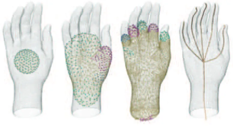
Cao et al. [Cao et al. 2010] present an algorithm for curve skeleton extraction via topological thinning to reduce the skeleton structure to a line, see figure1.32(b) and (c). This work is based on Au et al. [Au et al. 2008] but the method per-forms directly on point cloud data instead of the mesh domain. The algorithm first contracts a point cloud to a zero-volume point set. The contraction maintains the global shape of the input model by anchoring points chosen by an implicit Laplacian
smoothing process. Correct parameters tuning will result in a contraction which well approximates the original geometry of the shape. Next, a skeleton graph is built by sub-sampling the contracted cloud and computing a restricted connectivity. The skeleton graph with uniformly distributed nodes show in figure 1.32(c). Finally, unnecessary edges on the graph, measured by minimum Euclidean length, are iter-atively collapsed until no triangles exist to build a curve skeleton. Figure 1.32 give the overview of this algorithm.
Figure 1.32: Overview of the algorithm. (a) Input point cloud(orange) and the contracted points (red) after 1 iteration. (b) Contracted points after 2-5 iterations. (c) Skeleton graph constructed by father-point sampling (light red points) with a fixed radius ball and connectivity (red lines) inherited from the local neighborhood relationship of the input points. (d) The final 1D curve skeleton after topology thinning.
Conclusion
This chapter introduced how to measure and represent a shape with points. This will be the basis of our work. In particular, the different categories of measurement technologies have been depicted. Our work will focus on laser scanners. First meth-ods on the processing of point sets were also described for instance to manipulate or reconstruct the shape or the skeleton of the measured object.
Plant architecture representation
In general, representation of plant architecture are used to model structure and functionning of plants. However, the meaning of the concept of plant architecture is variable according to the context or the application considered. For instance, Hallé et al. [Hallé et al. 1978] consider it as the architectural model of a tree species, i.e. a set of rules that describes the growth patterns of an average individual of species. For Ross [Ross 1981], plant architecture is a "set of features delineating the shape, size, geometry and external structure of a plant". Godin [Godin 2000] proposes a more general definition where plant architecture is any individual description based on decomposition of the plant into components, specifying their biological type and/or their shape, and/or their location/orientation in space and/or the way these components are physically related one with another. This last definition better suits the work presented in this thesis, where 3D structure of real plants are reconstructed. From a reconstruction, the goal is to produce a representation of the architecture of a plant as the shapes and spatial positions of the components of the plant, and the connectivity between these components.
The aim of this chapter is to provide guiding principles of the numerous plant ar-chitecture representations. In Section 2.1, we will introduced global representations where plants are represented by a unique and compact model. These representations consider the complexity of a plant at the lowest level. By contrast, detailed repre-sentations, described in Section 2.2, rely on specific decomposition of a plant into modules. These representations have been organized in this review into three classes: spatial representations, topological representations, and geometric representations.
2.1
Global representations
Due to the geometric complexity of plants, modules or organs of similar types of them can be reduced into one or a few compartments providing a simple and compact representation. Therefore, this first approach consists of representing the plant as a whole, not decomposed into modules. These global representations can be divided into two categories: envelope-based and compartment-based representations.
2.1.1 Envelope-based representation
The complexity of plant geometry can often be abstracted as global models represen-tating their crown. The crown shape of a whole plant is a simple representation and has been used in various contexts for studying plant interaction with its environment
(i.e. competition for space [Phattaralerphong & Sinoquet 2005] or radiative trans-fer in canopies [Cescatti 1997]), 3D tree model reconstruction from photographs [Shlyakhter et al. 2001], and interactive rendering [Reche-Martinez et al. 2004]. These envelope models were specifically designed to represent plant volumes. 2.1.1.1 Simple envelope
A simple geometrical description of an enveloping surface of the crown shape can be constructed using symmetrical solids such as cones, ellipsoids, cylinders, or a combination of these. Spheres or ellipses are used for instance to model light inter-ception by tree crowns [Norman & Welles 1983], see figure 2.1. The plant canopy is approximated by an array of ellipsoidal subcanopies that may be equally spaced, randomly spaced, or spaced in any desired manner. In Baker’s work [Baker 1995], cylinders, cone frustums or paraboloids are used to study the mechanical properties of plants.
The main limitation of such approach are the approximate description of crown asymmetry.
Figure 2.1: Simple envelope representation by a set of ellipses. This model is used to calculate the light interception of the tree
2.1.1.2 Asymmetric envelope
Asymmetric envelope, originally proposed by Horn [Horn 1971] and Koop [Koop 1989], then extended by Cescatti [Cescatti 1997] and Pradal et al. [Pradal et al. 2009], makes it possible to easily define asymmmetric crown shapes. These envelope models can adapt to various tree geometries based on the following parameters: total tree height, height at crown inserting and at the greatest width of the crown, crown radii in four orthogonal directions, and shape coefficients of vertical crown profiles.
In figure 2.2, this envelope model can be created using six control points in six directions and two shape factors CT and CB that control its convexity. To
Figure 2.2: Asymmetric hull parameters. [Pradal et al. 2009]
define height of the crown, the control point PT represents the crown apex and PB
represents the crown base. The radius of the crown is defined using the peripheral points P1 to P4. P1 and P3 are constrained to lie in the xz plane and P2 and P4 in
the yz plane. Then, the peripheral line L at the greatest width of the crown can be defined from such points.
A point p of L can be computed as
p = [rPicosθ, rPjsinθ, zPicos
2θ + z Pjsin
2θ]. (2.1)
Where Pi and Pj are consecutive points with i, j ∈ [(1, 2), (2, 3), (3, 4), (4, 1)],
and θ ∈ [0,π2) is an angle between Pi and Pj, and rPx = q
x2 Px+ y
2 Px.
Points of L are connected to the PT and PB. The curvature of the crown above
and below of the peripheral line L are described with quarters of super-ellipses of degrees CT and CB respectively. The super-ellipses quarters connected between a
point p of L and PT is formed as
(r − rPT) CT (rp− rPT)CT + (z − zPT) CT (zp− zPT)CT = 1 (2.2)
An equivalent equation is obtained for super-ellipse quarters using PB and CB
instead of PT and CT.
The shape factors generate different envelope shapes such as conical (Ci = 1),
ellipsoidal (Ci = 2), concave (Ci ∈]0, 1[), or convex (Ci∈]1, ∞[) shapes. Figure 2.3
shows the various tree geometries represented using asymmetric envelopes. 2.1.1.3 Extruded envelope
Birnbaum [Birnbaum 1997] proposed extruded envelope from an horizontal and a vertical profiles for plant modelling. In this approach, each crown is represented in two dimensions: the first one is obtained from the projection of tree crown on the ground (see figure2.4.A), and the second one is obtained from a lateral view of the tree. The vertical profile is virtually split into slices by horizontal planes (see
Figure 2.3: Examples of asymmetric hulls showing plasticity to represent tree crowns generated by PlangGL [Pradal et al. 2009].
figure2.4.B) or by planes passing through equidistant points from the top (see figure
2.4.C). These slices are used to map horizontal profile inside vertical profile and a mesh is calculated.
Figure 2.4: Extruded hull envelope contructed from a horizontal and vertical profile. [Birnbaum 1997]
In figure 2.5, generated from PlantGL [Pradal et al. 2009], illustrates the re-construction of extruded envelope by sweeping the horizontal profile H inside the vertical profile V . Given B and T are the fixed points at the bottom and top of the vertical profile respectively. Vl and Vr are open profile curves, left and right, with
their first and last points equal to B and T . A slice S(u) is thus defined using two mapping points Vl(u) and Vr(u). Its span vector
−−→
S(u) is set to −−−−−−−→Vl(u)Vr(u).
On the horizontal profile H, Hl and Hr, the left and right points, are defined.
A horizontal section of the extruded hull is computed at S(u) so that the resulting curve fits inside V (see figure 2.5.b and c). Finally, to map −−−→HlHr to
−−→ S(u), the transformation is a composition of a translation from Hl to Vl(u), a rotation around
the −→y axis of an angle α(u) equal to the angle between the −→x axis and −−→S(u), and a scaling by the factor k−−→S(u)k/k−−−→HlHrk.
The equation of the extruded hull surface is thus defined in [Pradal et al. 2009] as :
S(u, v) = Vl(u) +
k−−→S(u)k |−−−→HlHrk
∗ Ry(α(u))(H(v) − Hl) (2.3)
Figure 2.5: Extruded hull reconstruction. (a) Acquisition of a vertical and a hori-zontal profile. (b) Transformation of the horihori-zontal profile into a section of the hull. (c) Computation of all sections (d) Mesh reconstruction.
2.1.1.4 Skinned envelope
The skinned envelope, proposed by Pradal et al. [Pradal et al. 2009], is inspired from skin surfaces [Woodward 1988,Piegl & Tiller 1997,Piegl & Tiller 2002]. The basic idea of this approach is a process of passing a B-spline surface through a set of vertical profiles given for any angle around the z-axis (see figure 2.6).
Figure 2.6: Skinned envelope reconstruction. (a) The user defines a set of planar profiles in different planes around the z axis. (b) Profiles are interpolated to compute different sections. (c) The surface is computed. Input profiles are iso-parametric curves of the resulting surface.
Given a set of profiles {Pk(u), k = 0, . . . , K} positioned at angle {αk, k =
0, . . . , K} around the z axis. All these profiles Pk(u) are assumed to be non-rational
B-spline curves with common degree p and number n of control points Pi,k. A
vari-ational profile Q can be thus defined that gives a section for each angle α around the rotation axis (see figure 2.6.b). It is defined as
Q(u, α) =
n
X
i=0
Ni,p(u)Qi(α) (2.4)
where the Ni,p(u) are the pth-degree B-spline basis functions and the Qi(α) are a
variational form of control points. Qi(α) are computed using a global interpolation
method [Piegl & Tiller 1997] on the control points Pi,k at αk with k ∈ [0, K]. For
this, let q be the chosen degree of the interpolation such as q < K.Qi(α) are defined
as Qi(α) = K X j=0 Nj,q(α)Ri,j (2.5)
where the control points Ri,j are computed by solving interpolation constraints
that results in a system of linear equations:
∀i ∈ [0, n], ∀k ∈ [0, K], Pi,k = Qi(αk) = K
X
j=0
Nj,q(αk)Ri,j (2.6)
Geometrically, the surface of the skinned envelope is obtained by rotating Q(u, α) about the z axis, α being the rotation angle. Thus, it can be define as
S(u, α) = (cos αQx(u, α), sin αQx(u, α), Qy(u, α)) (2.7)
2.1.2 Compartment-based representation
Compartment-based approaches that decompose plants into two or more compart-ments are intended to model exchanges of substances within the plant at a global scale [Godin 2000]. The core of such approaches is the description of how substances transfer within the plant. A compartment can be various elements such as leaves, roots, fruits or wood with connections between one another. The topological de-scriptions of the plant architecture for these models are very simplified due to the small number of compartments defined. In some cases, additional compartments can be included in order to refine the modelling of element exchanges within the plant.
The first compartment models have been introduced to model the diffusion of assimilates in plants [Thornley 1969, Thornley 1972]. These models describe transport-resistance availability of substances between leaf and root compartments. In figure2.7.a, a stem compartment can be added, for instance, to model the growth process of the stem and to take into account the consumption of assimilates in the diffusion process [Deleuze & Houllier 1997].


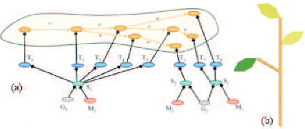
![Figure 2.13: Illustration of a multiscale tree graph. The decomposition of all vertices is not shown for readability reasons [Ferraro 2000]](https://thumb-eu.123doks.com/thumbv2/123doknet/14051322.460184/54.892.240.678.478.761/figure-illustration-multiscale-decomposition-vertices-readability-reasons-ferraro.webp)