Alternative methods of oil supply forecasting

M.A. Adelman and H.D. Jacoby

M.I.T. World Oil Project

Working Paper Number MIT-EL-77-023WP August 1977

1. THE ROLE OF "PRICE-TAKER" SUPPLIERS IN THE OIL MARKET

Analysis of likely developments in the world oil market is ultimately dependent on some method of forecasting oil supply from key regions.

Unfortunately, data problems tend to dominate work in this area, and much of the analysis task reduces to making the best use of the limited infor-mation that is available. Here we report on two alternative approaches to this forecasting problem, both avowedly data-oriented.

Petroleum exporters need to be grouped into two rough categories. First, there are what we will call "price-taker" suppliers. This is a group of petroleum exporters who appear to act as price-takers in the sense that each takes the world price (which is being set by others) as given. Each makes supply decisions according to his own parochial interest, without concern for their impact on the world price. This

*

This paper represents a collective effort by the Supply Analysis Group of the M.I.T. World Oil Project. Included in the group are

Professors Gordon Kaufman (M.I.T.) and Eytan Barouch (Clarkson College);

Dr. Paul L. Eckbo (Norwegian School of Economics and Business Administration); and research assistants James Paddock, James Smith, and Arlie Sterling.

An earlier version was given at the International-Energy Agency's Workshop on Energy Supply, November 1976.

The Project is supported by the U.S. National Science Foundation under Grant No. SIA75-00739. However, any opinions, findings, conclusions or recommendations expressed herein are those of the authors and do not necessarily reflect the views of NSF.

group includes non-OPEC sources of the North Sea, the USSR, China, and Mexico. It also may include members of OPEC who have low per-capita incomes such as Algeria, Indonesia, and Nigeria. Second, there is the

"cartel core"--a small group of nations who are the price-makers. This core includes Saudi Arabia, Kuwait, and others on the Arabian Peninsula; it also may include Iraq, Iran, Libya, and Venezuela. These countries

face a residual demand for world oil, which is the total demand less that supplied by the price taker exporters.

These groupings are not hard and fast; indeed a major focus of our inquiry is the circumstance in which a given exporter would change from one to another camp. The world oil scene is a dynamic interplay among these

importers and suppliers wherein the oil price is set by the members of the cartel core, who assume the task of controlling oil production so it does not outstrip the world demand forthcoming at that price.

In this paper our focus is on the price-takers. And, since the

desired form of a supply function depends on its intended use, we begin with a brief look at the broader market studies for which these supply

analysis methods are designed. The structure of the overall study is shown in Figure 1; the figure also is a simple flow diagram of the simulation model framework we are using to tie the various pieces of work together. The heart of the project is the supply and demand studies shown in the middle of the figure. These studies seek to improve our understanding

of the fundamental market forces, and to provide estimates of supply functions for price-taker suppliers and demand functions for importers. These functions are then incorporated into a simulation model of overall market performance.

An overview of the research method, and the results of the early simulation studies, are shown in the work of Eckbo [8].

0

L O E

r

.

0

a) U. .t; -·d a) .6

o- E

c

.

0

o

0

C

> C

a

O o

3a->

0

W 0 >4-a.E

O

o

C) I..

0

()

₀

4-0

The simulation framework is designed to accept an anticipated oil price trajectory, and to compute the resulting demands, supplies, and other market characteristics over the study period. Hypotheses about likely cartel price behavior are developed using a separate set of

1

behavioral models, as shown in the cloud at the upper left of Figure 1. Thus we approach the problem with two types of models--analytical representations of cartel behavior, and a detailed simulation of market supply and demand. The reason for the division is analytical convenience. The determinants of import demand and price-taker supply are varied and complex; they involve cost and price, along with the effects of tax and regulatory policies. To analyze the likely response of the market to one or another price pattern, one needs a method that can accept unwieldy

functional relationships. This requirement leads to a simulation framework for the overall analysis of market demand and supply outside the cartel. On the other hand, study of the cartel itself, and its pricing decisions, often involves some form of static or dynamic optimization calculation. For this part of the analysis, drastically simplified supply-demand

relationships are needed so that many formulations of cartel behavior may be simply and cheaply tested. The two analyses feed one another, as shown in Figure 1.

In keeping with our emphasis on the underlying forces in the market, the simulation framework is based on what we call a "bathtub" approximation to the world oil market. That is, the market is treated as a single pool,

Examples of this type of model include those by Pindyck [18],

Hnyilicza, and Pindyck [10], and Cremer and Weitzman [7]. Price scenarios based on judgment or the analysis of others also can be tested using the

simulation framework.

where exporters put oil in and importers draw it out. The details of the transportation network and the refinery and distribution sector are

almost neglected. Our aim is to match demand for products with the supply of crude, treating the intervening margin as a buffer, exogenously

determined. Data and simple models of these factors are part of the simulation framework, as shown in the two boxes at the left of Figure 1. We plan to add more complex representations of these subsectors only

as necessary.

The result of the overall simulation calculation is a forecast of net demand for oil produced by the cartel core--supplemented by work on core country supply, which is part of the overall supply-studies effort. Together, these components form the basis for study of current market characteristics, and forecasting of possible future developments.

The estimation of price-taker supply is a critical aspect of this analysis, and it is to this topic that we now turn.

2. PROBLEMS OF SUPPLY ANALYSIS

Several types of analysis have been used to explain and forecast

petroleum supply. One approach that has gained acceptance in recent years, particularly in the United States, is the use of econometrics. This

technique has been applied in circumstances where hundreds of large

fields, each containing a number of reservoirs, have given the productive systems the stability of large numbers, and where the depletion effect

(tending to raise costs as less of a reserve remains) has for a long time been offset by new discoveries and improvements in technology. Recently

this balance seems to have been lost. Also, in the data used in the econometric studies there seems to have been some ambiguity about the meaning of reported "reserves" and changes therein, so that a given year's reported "discoveries" bore little relation to what had actually been found. Moreover, there was no explicit attention to costs, which might cause a given price to be profitable in one place but not in another.

In studying supply from many areas of the world, the conditions for econometric analysis are even less favorable than in the U.S. In

many countries the oil fields are both fewer and younger, and even the short histories are poorly documented. Another limitation is the fact that the price series are so fragmentary and untrustworthy. The so called "posted prices" of the past were rendered meaningless around 1960, when they became

artifacts used for the calculation of taxes. Moreover, data on arms-length

1

sales of crude oil are insufficient and are ridden with too many errors to serve as a basis for econometric investigation. Were those problems not serious enough, current prices are far outside the historical range, and the inputs needed for development are not necessarily available in easy supply, either at constant or predictably changing prices. Finally, econometric calculations assumed, correctly, the existence of a competitive industry in the United States, hence a competitive supply curve. But our task is the modeling of a cartel, where price changes may have perverse effects on output.

Another approach to supply forecasting, which also involves an

orderly summation of the past, is that typified by the work of the National Petroleum Council [15], and subsequently applied by the Federal Energy Administration [20]. Under this approach, the experience of past

exploratory drilling is summarized and a trend in the finding of reserves per fot drilled is established. Based on estimates of the costs of

exploration and development, calculations are made of the relative attractive-ness of exploratory activity, conditioned on some assumption about the price of oil. Given an estimate of exploratory drilling, the forecast of barrels added per foot drilled, a reserve-to-production ratio, and hoped-for

stability in reserve expansion in old "fully-developed" fields, it is possible to forecast supply into the future.

Unfortunately, many of the shortcomings of the econometric approach apply as well to the NPC-type format. In many areas of the world the

exploratory histories are poorly documented, and several of the relationships which are required for this approach may be estimated only very approximately.

new, and the experience that makes the NPC method believable simply does not exist. Moreover, the more productive potential areas in the world often are located in offshore or otherwise inaccessible areas, and the cost of development-production of particular resources weighs very heavily in the supply relation, as opposed to the phenomenon of exploration and finding which is emphasized in the NPC method.

Finally, there are the methods of resource estimation used by

oil companies in evaluating prospective areas, and in constructing global estimates of regional or world resources. These methods, which draw on detailed geologic and geophysical data as well as on past drilling exper-ience, seem to be rarely used for supply estimation of the type being carried out here. Where they are so applied, it usually is nrt possible to gain access to the details of underlying data and assumptions. They do,

nonetheless, contain important components of concept, information and analytic method, and use is made of these approaches below.

2.1 Key Factors in the Analysis

To a very great extent, therefore,the mechanisms we have chosen to use are determined by what we perceive as the severity of data limitations in the main variables. The first and fundamental problem is in the reserve data. Viewed as an economic process, oil supply is the depletion of a stock, which is constantly being renewed by adding new reservoirs and expanding the

limits of the old ones. "Reserves" have for years been reported by The American Petroleum Institute (API) for the United States on a

consistent and meaningful basis [1]. Essentially they represent "money in the bank": in effect, the organized consensus of industry personnel as to the amount to be produced from existing installations. Elsewhere,

one must rely on government estimates whose basis is rarely revealed, and on the trade press, which also is essentially an informal consensus of company opinion. The main difficulty in using non-API estimates results from various conceptions and definitions of what is likely to be added, how soon, to "proved reserves." In all cases, "reserves"

are not a direct measurement but an inference drawn from data on geological structure plus observations on production volumes, pressures and tempera-tures. There will be legitimate differences of opinion in the interpreta-tion of such data, hence in the estimainterpreta-tion even of "proved" reserves. These variations are magnified as one moves from reserves proved to those considered as "probable" in the existing cluster of reservoirs.

A considerably greater leap, and the one calling for more specialized knowledge, is the estimation of "undiscovered reserves." Less than

a decade ago, such estimations were an exercise in method; or in the language of a distinguished geologist, Lewis Weeks, they were merely an indication of where an exploration department ought to go look. These estimates had, in short, only a relative meaning, and it was a plain error to compare them with, or add them to, proved or probable reserves in known reservoirs. But today one can estimate the ultimate reserves for a "trend" or "play"

(i.e., a population of reservoirs, generated by a geological sequence) provided that enough is already known about the area to furnish a reliable sample. Such a method is presented in Section 3 below. The combination of mathematical statistics and geologists' knowledge is not easily

created, however, and we have been able thus far to apply the method in only one area, the North Sea. A number of estimates have been made, much more approximately, for larger areas. These are discussed in Section 4.

Rather than rejecting or ignoring them as not good enough, we regard them as a considerable advance on simple extrapolation on the basis of cubic yards of sedimentary rocks, etc.

An equally important data limitation is from reservoir engineering: how much can be produced out of a given set of reservoirs in any given

time. In the past few years these limits have been perceived as much more tightly binding. When the price of oil in the United States was

around $3 per barrel there was little dissent from the view that if the price were $6, vast new reserves could be created by applying more capital and extracting much more than the average 30 percent of the oil in place.

These hopes are not dead, but it is now seen that too little was known Of the processes by which additional oil could be recovered from a given reservoir, in the field rather than the laboratory. In the United States, drilling has responded to price, but reservoirs have not.

There also has been some unpleasant learning about the amount which can be produced per day or per year without damaging the reservoir and lessening the ultimate recovery to the point where present value is also less. Iran is one example. We happen to have obtained the capital bud-gets of the Iranian Consortium for over a decade [6]. Reading them in succession makes it plain that for years there was no felt need to know what would happen if production were raised by several times. It was reasonable to foresee, at prices much less than now rule at the Persian Gulf, capacity of 10 million barrels daily (mbd). The maximum will probably be a third to fourth less. Instead of a continuum, with higher prices

bringing out higher output rates, the marginal cost appears to become nearly vertical in the neighborhood of 6 to 7 mbd. Given the strategic

position of Iran among oil producing nations, this change has had impor-tant consequences. We can only be sure it is not the only one nor the last.

Finally, there is the influence of government policies. In competitive industries, supply and demand will be equated by price; in non-competitive industries, by marginal revenue. World oil is a good deal more complex. At current prices, the margin of price over costs is very great even in the highest-cost areas. Where the industry is operated by private

companies, payments to the government greatly exceed payments to factors, including capital charges. Hence the most important economic variable, sometimes by factors of 10 or even 100, is the government's perception of how great a rent exists, and how high a price they can charge without reducing their total take. But the government take may also be in the

form of participation or joint control. There is much room for misunder-standing and deadlock, so that a given country's actual rate of development may be much bellow where it would be under a government which was better

informed and free to maximize, without political or ideological pressures. Matters are simpler in those countries where the oil industry is owned entirely by the government. As a first approximation, given knowledge of development costs and of known and probable reserves, one can calculate the

rate of output which would maximize the present value of the current reserves--as well as estimate the finding rate which maximizes the present value of reserves in reservoirs to be discovered in the known areas. But

one may need to modify the approximation to accomodate cartel solidarity, or other objectives.

In some countries, there is a backward bending supply curve, where

to take such different cases as Canada and Malaysia. Higher prices may promise to generate so much revenue as to disrupt the desired rate of social adaptation; as a result, the higher the price, the less

the target rate. A government with certain plans or obligations can meet them, given higher prices, with less output; hence is willing to reduce output or at least to accept reductions. Finally, price increases always

generate expectations of still further increases. This raises the present perceived value of any reserves, and lowers the optimal rate of development.

Thus the three basic determinants--reserves, development costs, and government policies--must be put into a framework where they can be acted upon by current and expected prices. The framework must be modular to an extreme degree, since there is hardly a piece of the data base which we may not need to replace at any time, as more becomes known, or as data become outmoded.

2.2 To Approaches to Price-Taker Supply

Here we present two of the analysis methods that we are exploring. One of these, the "'disaggregated pool analysis," is the most detailed of the models developed and requires the most data, geological interpretation, and computational capacity. The other, which we call "aggregated country

analysis" is among the most simple of the methods formulated. Various extensions, modifications, and combinations of the two approaches remain

to be explored.

Though one approach is far more ambitious than the other, essentially they are variations of the same model. That is, the supply function is based

within a petroleum region. Both take account of geological data, though one has a more complex hypothesis about geological deposition and the nature of the exploratory process. Both take account of economic factors such

as costs and future petroleum prices, and both include an approximation of oil-developer decisions, though the aggregated method necessarily treats

these in a highly summarized manner. Both allow for the effects of

tax regimes and other aspects of producer country oil policy, though once again the details of tax structure must be sacrificed in the aggregated model.

Figure 2 shows how the two analyses fit into the sequence of activities which compose the oil production industry, and the kinds of statistics

generated. Looking first at the left-hand column, an immense store of experience, combined with formal science and technology, gives rise to judgmental estimates of what may be contained, and is worth producing, in various parts of the world. The unknown areas are judged by analogy with the known. The kinds of pools which may be generated and the relative size distributions, constitute the estimates of "ultimate production," as compiled by several oil companies.

These estimates have a direct effect on the direction of geological and geophysical prospecting. The knowledge gained thereby feeds back into the judgmental estimates. Geological-geophysical results also determine exploratory drilling, in new and in old areas; and the good or bad results again feed into judgmental estimates, both of "ultimate production," and of what may be thought, in old areas, of likely new discoveries there, i.e., "probable reserves."

Exploratory drilling generates dry holes, which are not necessarily bad news, since the information about successive layers may be of great value;

ACTIVITY "RESERVES"

Accumulating fund of geological .knowledge, areas considered

promising and unpromising, by

types and amounts of sediments.

Unknown areas appraised by

analogy to known ones.

Judgmental estimates of

accumulations and size

distributions.

:_:_;___*_______________ "Ultimate Production"

Geological and geophysical

analysis, old and new areas.

Exploratory drilling, old

and new areas.

Discoveries, old areas and

new basins, fields and pools.

Development .

Production

*

}->iiii~i{iiiii "Probable Reserves"

I

."Proved Reserves"

"Producing Capacity"

H

Aggregated Country Analysis

Figure 2. Sequence of Oil Activities and Kinds of Statistics Generated

Disaggregated Pool Analysis

.... m&___ . ... Audi P v CII.e I·~~ - .. -..-..-... l ...- · )oi···--;::-, L~~~~~~~~~~~~~~~~~ 7it · · :;·:· I I

it also leads to new fields in old areas, again affecting estimates of "probable reserves" and, perhaps more weakly of "ultimate production."

At this point the Disaggregated Pool Analysis can begin. Given enough wells drilled to furnish a reliable sample, and given geological knowledge to

certify the existence of a population from which the sample is drawn, a forecast is made of the underlying distribution, the number of reservoirs to be found, and their size distribution. Given knowledge of costs, prices,

and tax policies, one can make a forecast of the rate of exploratory drilling, and the rate of development of the area.

Stated in terms of the steps of our analysis procedure, the disaggregated pool approach is shown in the left half of Figure 3. First, an

estimate is made of the number of exploratory wells in the region.

Then the exploratory process itself must be approximated, and an estimate made of the number of reservoirs found and their

characteristics--e.g., recoverable reserves, well productivity, depth to pay, and (in the case of offshore areas) water depth and distance to shore. The key variable is recoverable reserves, and here the method draws on research on statistical analysis of the exploratory process carried out by

Kaufman and Barouch 2,3]. The economics are then calculated, reservoir-by-reservoir. Development costs are estimated from the reservoir characteristics and applicable tax rules, and these are combined with an evaluation of

revenues based on expected oil prices. Built into the analysis is an evaluation of the likely production profile for reservoirs with different characteristics. The overall supply estimate for an area is the sum of the production profiles of its individual reservoirs; and the overall

supply from a country (or other region) is the aggregate of the results from the various areas distinguished for analysis.

0

-C

o

> - I C U) O'0

;

O

a1) Q Q)

cr-o

I-0

o

2>E

C0

0 ,o

_o

-0. U)

c

0

c

C') I) i >J

z

a:

z

0

w

w

(D (9 ._ cn

>-J

z

0

0

a

w

w

Q

U)

0

c) '4--0 4, C

0

_t

_rl

_c

L. =3 CP U-. o-

(n

-3

>

CL CL -0. Co E -OC 0 0,,- Q>

>

· -- a) WX .., NI.a- ',,--U O

E

a.

' Z

0 U) " U LU

o

_

C0 L. CL 1* 0 U, > @ C) w)0 wro

_a)

QM D 0) '4- TrC .t o >% W

c

. cc

_ o.E

4- a C x2 1

W W

C

, nb

>a

_ t

C o

- Q. ) X U)o O.

0

0

cn- o.

%-The disaggregated pool analysis is a formal, precise, reproducible version of what happens in industry every time a discovery is made. Estimates of probable reserves are changed, as well as of "ultimate production." As development wells are drilled, providing new producing capacity and more detailed knowledge of reservoirs, the forecast of their production is crystallized into the industry estimates of "proved reserves."

The aggregated analysis is an attempt to tap into the calculations which the industry has already made, which are in substance the same as the

disaggregated pool analysis. By considering prices, costs, and taxes, the companies have already made estimates of what they expect to produce. Recent experience indicates how fast a given amount of drilling effort will produce the associated productive capacity, i.e. the ability to

deplete a given reservoir in a given length of time. And the "probable reserves" and "ultimate production," both affected by recent experience, are imprecise measures of the larger "pool" out of which are being

impounded the newly "proved" reserves. The smaller the proportion impounded up to the present, the more is left to be taken into "proved reserves"

before rising marginal costs are felt. This is strictly analagous to

the discovery decline rate which is made explicit in the statistical analysis at the pool level.

Once again, the approach can be expressed in terms of the explicit steps to be worked out in Section 4. As indicated in the right-hand panel of Figure 3, exploratory and development activity are measured in

rig years for the area in question, and an estimate is made of proved reserves added per rig year. Instead of making a detailed study of reservoir economics, we factor in the industry's estimates, since all

proved reserves are by definition slated to be developed. The focus is on the amount of capacity that will be installed, considering costs and expected oil prices. The cost data are not in the form of cost functions, as required by the disaggregated model, but simple estimates

for each country of the capital coefficients per daily barrel of

capacity and of operating cost per barrel of production. As with the disag-gregated analysis, separate estimates are made of supply from reserves

already in production, as shown in the lower part of the diagram. And, of course, the method is flexible enough to take account of information about other aspects of planned activity.

Both methods are based on the same idea of how reservoirs are

distributed in the earth and on the same sequence of industry operations. Whether we use one or the other depends altogether on the available

data on the one side, and the money and manpower available to use them, on the other.

3. DISAGGREGATED POOL ANALYSIS

As noted above, the key to the disaggregated method of forecasting is the statistical analysis of the exploratory process, and economic

evaluation of the pools that are found.l Methods have been developed whereby a forecast can be made not only of the total recoverable reserves

to be discovered by a given level of exploratory effort, but of the distri-bution of pool size itself and of the sequence of discoveries by size. Pool size is a key to the economics of supply, particularly in offshore areas (or under certain tax regimes) where small pools (and under some

conditions relatively large ones) may be uneconomic to develop. Pool size also is a significant influence on the speed of development and the

time profile of production from reserves that are economic to produce.

3.1 Analysis of the Exploratory Process

As currently implemented, the analysis begins with a postulated level of exploratory effort within an oil "play." A play is defined as the pre-drilling and drilling exploration of a geological configuration, generated by a series of geological events, and conceived or proved to dontain hydrocarbons. The wells drilled form a statistical population. An important element of the research is to discover the difference in

1

What follows is an abbreviated version of the disaggregated method. Its development and initial applications are described in a paper by the M.I.T. World Oil Project [19], and the methodology is further developed in a paper by Eckbo, Jacoby, and Smith [9].

results that may accompany alternative ways of drawing these geographical boundaries. For example, the North Sea results shown here treat the entire region as a single play, but work is under way to perform the same

analysis with the area divided into four areas that correspond more closely to the geologist's definition of a "play."

Exploratory effort is measured in terms of the number of exploratory wells, Wt, to be sunk in period t. To this drilling effort we apply

a "dry hole risk," 6t, which is the probability that an exploratory well will fail to find a field. For purposes of the example developed

here, 6t, is held constant over the forecast period, and reflects a judgmental estimate based on historical experience. The expected number of discoveries

in a period can then be expressed as Wt(1 - 6t). The purpose of the analysis of the exploratory process is to determine the expected charac-teristics of the next set of discoveries in a petroleum play over some period to be analyzed. This is the first step in calculating the

contribu-tion that new pools may make to future supply, as shown in Figure 3. This estimate can be combined with data on pools already discovered to produce an overall supply forecast for the play.

The analysis of the exploratory process is based on two hypotheses about the natural process of resource deposition. Following the work of Barouch and Kaufman [2,3], one assumes that the number of pools in a play, N, and their size distribution (characterized by the mean and variance, and a ) are generated according to a probability law whose functional form

is dictated by the way in which nature deposited the oil in the

first place. Many distributions may be analyzed using the methods applied here, but the customary assumption is that pool size in terms of recoverable reserves, r, is a random variable, and that its density function

normal ; i.e., log r is normally distributed with mean i and variance a. To this hypothesis about nature, then, is added another hypothesis about the process by which oil operators search for and find these

reservoirs. Once again following the work of Kaufman and others [2,3] the exploratory process is characterized as one of random sampling, without replacement, in proportion to pool size, r. With these hypotheses

it is possible to predict the characteristics of discoveries number n+l, n+2,..., N--and also total recoverable reserves in the play,

N

E r. -- if we know there have been n discoveries of size rl,...,r

j=l 3

and the order in which they were discovered.

The procedure is as follows. We can specify joint distribution function of the n discoveries to date conditional on the parameters ,a , and N:

2

D(rl,

.,

r

,

a ,

N)

(1)

Then, using the actual sequence, rl, ..., r as one sample from this

n

distribution we can estimate (using maximum likelihood techniques)

the parameters , a2 and N. Table 1 presents the sequence of discoveries in the North Sea, which we use as the basis of the sample calculations pre-sented below.

Next, it is possible to specify the density function of discovery number n+l conditional upon the exploratory history already experienced,

^2

rl, ..., r , and given estimates of the parameters i, a , and N. This

n

The estimates are treated as measures of "proved" reserves, although the strict conditions for such a definition often have not been met (i.e., limiting the estimate to reserves-actually enclosed.by development wells). 'The assumption is that a small number of exploratory and development wells,

when coupled with geophysical data on structure size, gives a reasonably accurate estimate of what will ultimately be proved in a given specific reservoir.

Table 1. Northern North Sea Discoveries, Recoverable Reserves Oil Equivalent (Millions of Barrels).

Name or

Order Location Date Size

1 Cod 2 Montrose 3 Ekofisk 4 Josephine 5 Tor 6 Eldfisk 7 Forties 8 W. Ekofisk 9 Auk 10 Frigg 11 Brent 12 Argyll 13 Bream 14 Lomond 15 S.E. Tor 16 Beryl 17I cormorant 18 Edda 119 Heimdal :20 Albuskjell

i e_]_^

2/68 4/69 9/69 6/70

8/70

8/70 8/70 8/70 9/70 4/71 5/71 6/71 12/71 2/72 4/72 5/72 6/72 6/72 7/72 7/72 _ ,__A 156 180 1713 100 243 910 1800 490 50 1325

2500

70 75 500 34 525 165 98 300 357 Name or

Order Location Date

31 Ninian 32 Statfjord 33 Odin 34 Bruce 35 Magnus 36 N.E. Frigg 37 Balder 38 Andrew 39 Claymore 40 E. Magnus 41 9/13-4 42 15/6-1 43 Brae 44 Sleipner 45 Hod 46 211/27-3 47 Gudrun 48 2/10-1 49 3/4-4 50 14/20-1 51 Crawford 52 9/13-7 53 3/8-3 54 Tern 55 21/2-1 56 3/2-1A 57 Valhalla 58 3/4-6&3/9-1 59 15/13-2 60 211/26-4 9/73 12/73 12/73 3/74 4/74 4/74 4/74 4/74 4/74 6/74 6/74 9/74 9/74 9/74 11/74 11/74 11/74 11/74 12/74 1/75 1/75 1/75 1/75 2/75 2/75 3/75 4/75

Source: Beall [4], and estimates by the M.I.T. World Oil Project as of June 1976. Size 1000 4960 178 450 800 71 100 300 375 250 220 150 800 50 75 450 450 100 100 i 75, 150 350 100 175 175 200 50 200 200 175 I i . _ . _ _ _ _

we may write, defining r = (rl, ..., r), as

-- n

D(rn+l r; , N). (2)

st

r has been observed, is

E(rn+1 r) = f xD(x r; , , N)dx. (3)

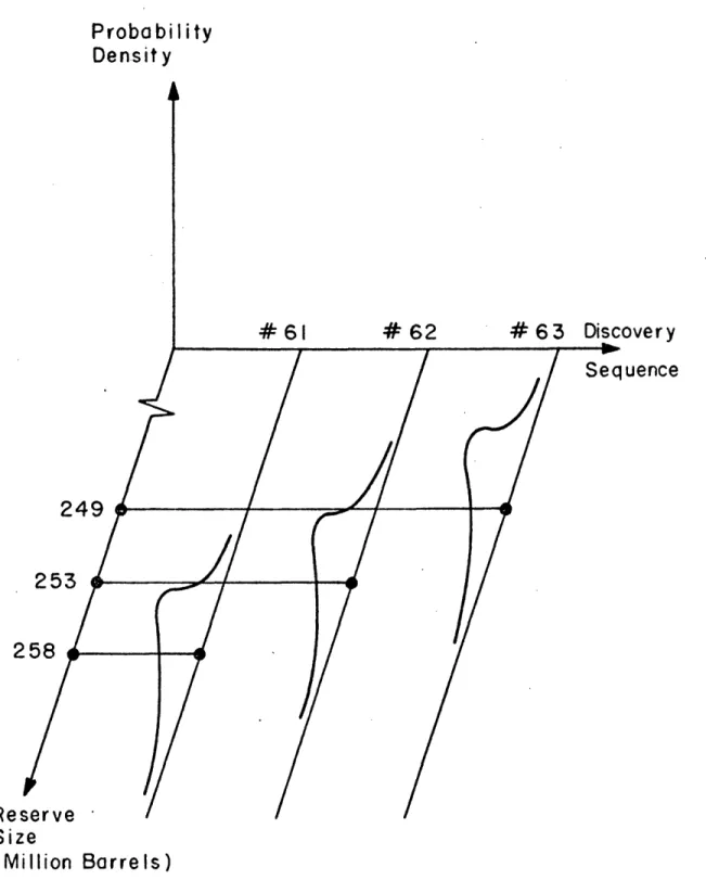
The nature of this calculation can be seen in Figure 4, based on data from the North Sea. When this analysis was done there had been

60 discoveries in the North Sea, so n = 60. The figure shows the rough shape of the density function for the 61st discovery along with the conditional

expectation E(r6 1 r) of the size of the 61st discovery, which in this

case was 258 million barrels. The calculation for n+2, n+3, etc. is a straightforward extension of this procedure.

One further step is necessary before proceeding to economic

and financial analysis of the reservoirs themselves. As stated earlier, smaller pools may be uneconomic to develop, and the pace of extraction may differ among larger pools depending on size. Therefore we need some indication of the expected number of barrels to be found in pools of

various sizes. The data for such a calculation is contained in the conditional distribution of Equation 3, and using this function we can calculate the

partial expectations of the numbers of barrels in reservoirs of various sizes. To do this we define a set of k class sizes S_k, where the size limits are defined as shown in the following table.

Probability

Densit

y

#61

uence

249

253

Rep

Size

( Million Barrels)

Figure 4 The Sequence of

overy

2

Class (k) Lower Limit Upper Limit

1 a1 a2

2 a2 a3

3 a3 a4

Then for the (n+l)st discovery the expected number of barrels to be found in pools in size class k, or the partial expectation of size class k, is

2+1

= J xD(x N)dx (4)

n+l,k

d

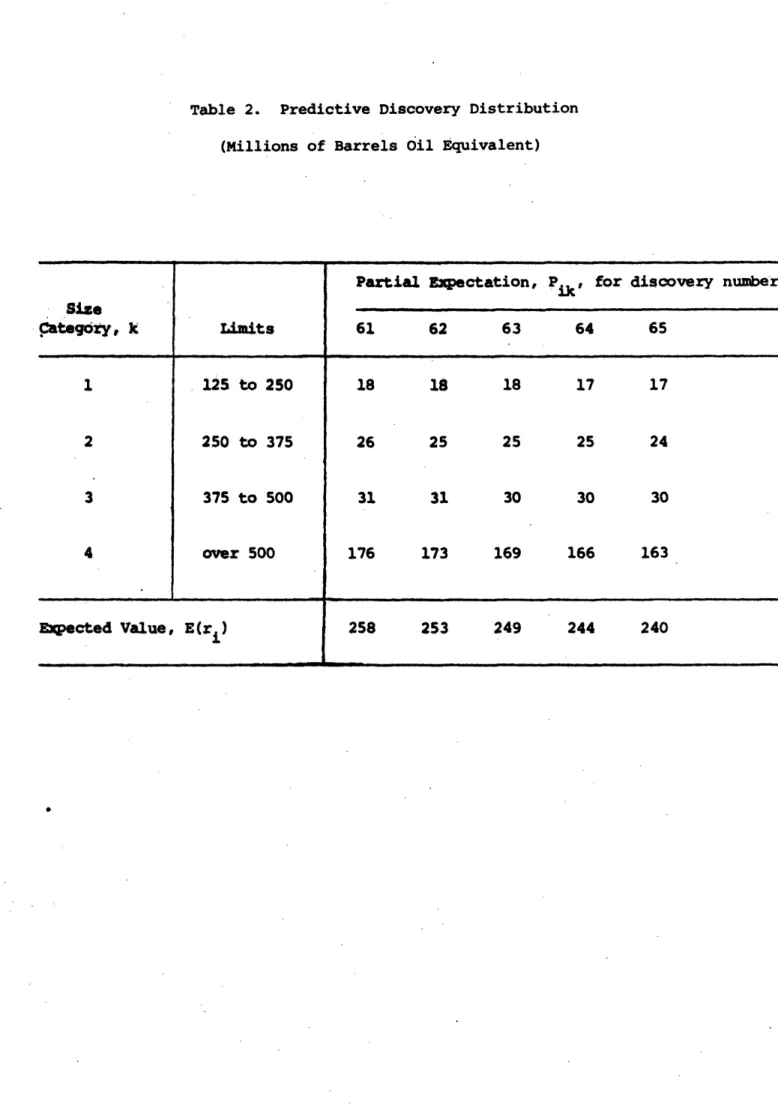
The results of this calculation are illustrated in Table 2, once again using data from our North Sea example. Four size categories are used and the table shows the partial expectations of the number of barrels to be discovered in each category in the next five successful exploratory wells.

Though the table shows only the first few discoveries from a longer

sequence that must be generated for supply forecasting, several characteristics of the process are evident in the data shown. First., most of the oil is

expected to be found in larger reservoirs, and the difference in economic reserves which would result were the smaller size reservoirs infeasible

to develop is not great--though it is significant. Second, the table plainly shows a process which we refer to as "discovery decline." That is, as the province is drilled up, the expected findigg from each additional

success-Table 2. Predictive Discovery Distribution (Millions of Barrels il Equivalent)

Partial Expectation, Pik for discovery number

Size

Category, k

Limits

61

62

63

64

65

1 125 to 250 18 18 18 17 17 2 250 to 375 26 25 25 25 24 3 375 to 500 31 31 30 30 30 4 over 500 176 173 169 166 163

Expected Value, E(ri)

258

253

249

244

240

ful exploratory well tends to decrease. This is the behavior one would expect in practice, and it falls out of the analysis because the funda-mental geological facts of life are built into the method through

the two key hypotheses introduced earlier.1

Referring again to Figure 3, the results in Table 2 constitute the data on "reservoirs discovered." The next step, then, is to estimate what will be done with them once their location and size are known.

3.2 Evaluation of Reservoir Economics

There are a number of attributes of an oil reservoir that influence its economics. The most important is recoverable reserves, and this we predict by the methods above. Reservoir depth and (in offshore areas) water depth and distance to shore also are imporant determinants of

cost--though these usually do not vary significantly over a region of the size on which this analysis is based. Likewise, average well productivity is an important factor, though it also is reasonably assumed to be

constant over the unit of analysis when a relatively disaggregated approach is taken. These attributes--together with cost factors, tax rules, and the expected oil price--determine the economic viability of a reservoir.

A similar phenomenon is built into the aggregated analysis as well, where the amount added to reserves is a decling function of the number of rig years in an area.

Note that the discovery process has been defined in terms of recoverable reserves, and the analysis of Equations 1 through 4 carried out apart from concern for the oil price. In principle, the amount of oil that is "recoverable" from the oil in place is a function of price and

cost factors: at higher oil prices it is worthwhile to spend more to recover a larger percentage of the oil. In practice, given the state of the art at any moment, and in the relevant range of prices, elasticity of recovery factor to price appears to be very low.

We are concerned here with the behavior of price-taker suppliers, and in particular with the forecasting of their response to the price strategy of the cartel core. Since smaller reservoirs are more expen-sive to develop, per barrel produced, one may expect that higher cartel prices will bring more resources to the point of economic viability and call forth increased price-taker supply. To analyze this phenomenon, we construct a cash-flow analysis of the reservoir from '_he operator's viewpoint.

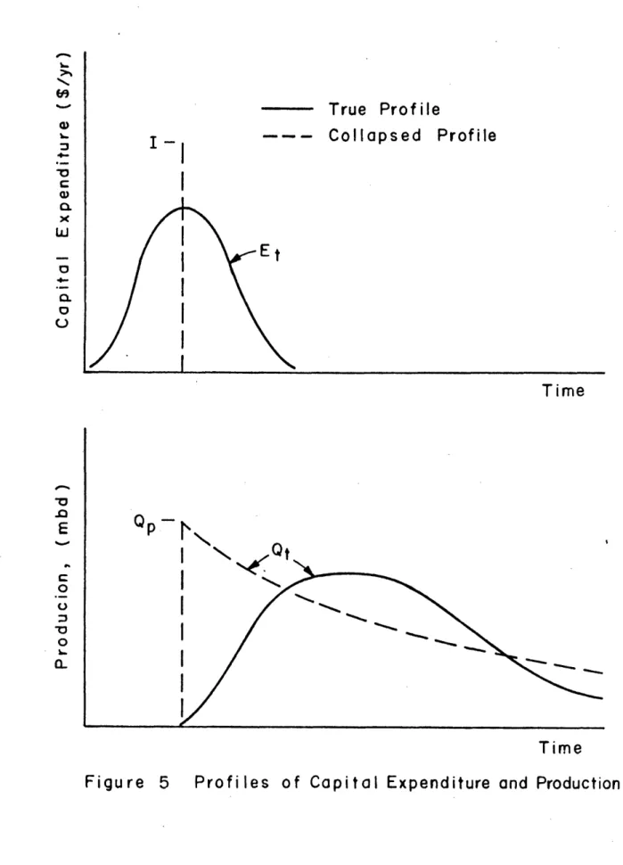
A profile of capital expenditures typical of oil reservoir develop-ment is shown by the solid line Et in the top half of Figure 5. We have

prepared an analysis of reservoir economics to generate estimates of E_t for reservoirs of different size [9, 19]. Relationships were estimated for the various components of capital cost (e.g., development drilling,

platform structures, platform equipment, pipelines, terminals) and of operating cost. In this analysis of the North Sea, extensive use was made of

data prepared by Wood, Mackenzie, and Co. In addition, detailed consideration was given to the tax systems of the U.K. and Norway.

Estimates were also prepared of the typical patterns of annual production, Qt' from reservoirs of different size, as shown by the solid curve in the bottom half of Figure 5. These data are then combined into a cash flow analysis of reservoir investment and production, both to determine economic viability and to establish the likely production

profile, reservoir by reservoir. (The dashed lines in Figure 5 represent a simplified or "collapsed" version of development expenditures and

the associated production profile. The collapsed model is used in constructing the aggregated model of oil supply, discussed in Section 4.)

True Profile

Collapsed Profile

Et

Time

N

Time

of Capital Expenditure and Production

I-i

,I 4-a, .

c

x

a

h4 O.

0

'C

E

0

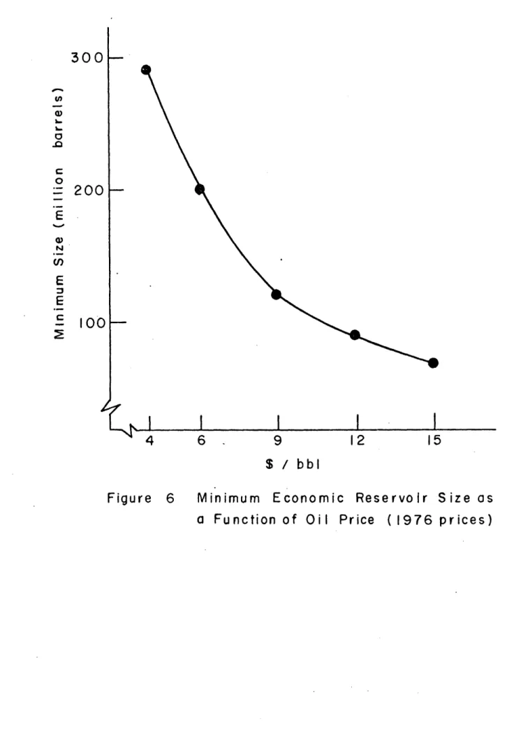
0= ' L n-l I I I I I I I,

The result of the reservoir analysis is shown in Figure 6, once again using data from the North Sea. The figure shows a plot of the minimum sized pool which it is feasible to develop given an expected level of oil price. At $6 per barrel (1976 prices), no reservoir below 200 million barrels will be developed given current costs and tax rules in the North

Sea. At a $12 price, the marginal reservoir decreases to 90 million barrels. Similarly, it is possible to hold price constant and calculate

the effect of changing tax rules.

3.3 Simulation of Supply

The analysis of the exploratory process, presented in Table 2, and the evaluation of reservoir economics, summarized by Figure 6, then constitute the building blocks for simulation analysis of' price-taker supply. Refer again to the left-hand side of Figure 3. Based on an estimate of exploration drilling activity (which for this example we estimate from announced plans) a discovery sequence generated. It represents the expected value of the reserves to be found in pools of various sizes. These expected quantitites are

then subjected to analysis of economic viability. Submarginal reservoirs are held aside until such time as rising oil prices or postulated revisions

in tax rules change their attractiveness for development. Those reserves that are in pools above the minimum pool size are then converted (based on analysis of reservoir economics) into a time profile of production. To the estimates of supply from new discoveries, then, are added data on expected production from reservoirs already in production or under development. These, of course, constitute the more accurate portion of any forecast. In the North Sea we depend heavily on Wood, Mackenzie data for these estimates.

4

6

9

12

$ / bbl

Figure 6

Minimum

Economic

Reservoir

( 1976 prices)

300

u, O.-La -_a) D a

0

U)N (n

E

C

2

200

100

4

15

Size as

,! ,& I I I I I

a Fu nction of Oi Price

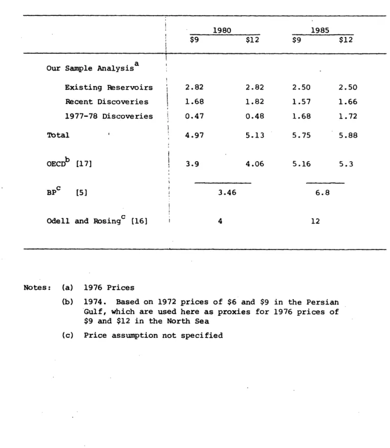
The final result is a supply forecast built up pool by pool for existing fields and (on an expected value basis) discovery by discovery for new reservoirs. If there is more than one play in the supply region, then the regional production is built up play by play. The resulting supply estimtes for the North Sea are shown in Table

Table 3. North Sea Supply Estimates (Million Barrels Per Day, oil equivalent)

1980 1985

$9 $12 $9 $12

a

Our Sample Analysis

Existing Reservoirs 2.82 2.82 2.50 2.50 Recent Discoveries 1.68 1.82 1.57 1.66 1977-78 Discoveries 0.47 0.48 1.68 1.72 Total ' 4.97 5.13 5.75 5.88 OECDb [17] 3.9 4.06 5.16 5.3 BPc [5] 3.46 6.8

Odell and Rosingc [16] 4 12

Notes: (a) 1976 Prices

(b) 1974. Based on 1972 prices of $6 and $9 in the Persian Gulf, which are used here as proxies for 1976 prices of $9 and $12 in the North Sea

4. AGGREGATED COUNTRY ANALYSIS

It is only in special circumstances where we have the data needed for the disaggregated analysis, so we are developing a greatly simplified, but consistent, aggregated method sketched in Figure 3. It is modular,

in that the estimates for any given country, region, or field can be replaced by more precise knowledge when available from other sources.

As noted earlier, the method is based on forecasts of rig activity and analysis of proved-reserves added per rig year. Reserve additions then become an input to calculations of capacity expansion and likely oil production. Therefore we turn first to the data sources for worldwide reserves, and the way they may be used to forecast new additions.

4.1 Analysis of Reserve Additions

As used by the American Petroleum Institute (API) the concept of proved reserves has a definite economic meaning: a highly accurate forecast of what will be produced from wells and facilities already installed. Since variable costs are normally only a small part of the total, it would take an unusually severe price drop to abort much

production. It is this concept of reserves that forms the basis of the model developed below.

However, outside the U.S. published "proved reserve" estimates generally include a substantial element of what the API calls "indicated additional reserves from known reservoirs." At end-1975 in the U.S.

(excluding Alaska) this category included 5.0 billion barrels compared with 22.7 billion proved reserves, or an additional 22% [1]. Usually the published "proved reserves" go farther. Interesting data were

gathered in a survey of oil companies conducted by the National Petroleum Council. The companies made estimates of the discrepancies between API "proved reserves" and the reserves as published by the Oil and Gas Journal

(OGJ). The results are shown in Table 4. Since the North Sea was insignificant in 1970, the close agreement on Europe is now outdated. Essentially, OGJ reserves for certain large Persian Gulf and African countries include a large amount of oil not yet developed into proved reserves, and the companies were not unanimous on its size.

We gain a different and more useful perspective on reserve estimation by noting that reserves credited to individual developed fields fall

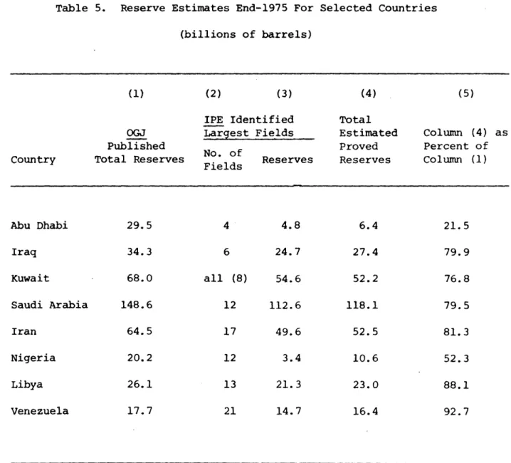
substantially below the OGJ national totals. Table 5 shows a comparison of OGJ data and estimates of the largest fields as published by the International Petroleum Encyclopedia (IPE), along with an estimate based on the IPE figures. The estimate of proved reserves (Column 4) was prepared by dividing IPE reserves of identified largest fields by the portion of total country production accounted for by those fields. Finds accounting for less than 3 percent of current production were excluded.

(In Lybia the proportion was based on cumulative not current production.) These authors' estimates as a percentage of the OGJ figure is shown in Column 5; the results are consistent with those in Table 4.

Prior to 1975, the percentages in column (5) would have been lower, since OGJ in that year revised its estimates downward, and for the first time labelled them "proved reserves" and stated that "probable and possible

reserves [are] not included." Given this definition, we should consider that the excess of OGJ reserves over those estimated on an IPE basis includes largely the undeveloped portions of known fields, including some known but undeveloped reservoirs. For our purposes, the IPE-based

Table 4. Oil Company Estimates of Proved Reserves (API Concept) As A Percent Of Published Reserves (Oil and Gas Journal), 1970

Proved Plus

Proved Probable

Area Reserves Reserves

Latin America .97 to .99

Europe .97 to .98 Not

Africa .50 to .73 Available

Middle East .67 to .80

Total .66 to .81 .88 to .97

Rough Point Estimate about .75 about .95

Source: National Petroleum Council Committee On U.S. Energy Outlook: an Interim Report. An Interim Appraisal by the Oil Supply Task Group, 1972, pp. 21-24.

Table 5. Reserve Estimates End-1975 For Selected Countries (billions of barrels)

(1) (2) (3) (4) (5)

IPE Identified Total

OGJ Largest Fields Estimated Column (4) as

Published Proved Percent of

Country Total Reserves Fields Reserves Reserves Column (1) Fields Abu Dhabi 29.5 4 4.8 6.4 21.5 Iraq 34.3 6 24.7 27.4 79.9 Kuwait 68.0 all (8) 54.6 52.2 76.8 Saudi Arabia 148.6 12 112.6 118.1 79.5 Iran 64.5 17 49.6 52.5 81.3 Nigeria 20.2 12 3.4 10.6 52.3 Libya 26.1 13 21.3 23.0 88.1 Venezuela 17.7 21 14.7 16.4 92.7

figures are preferred for they are closer to the API definition, though considerable judgment may be involved in making estimates for particular countries.

Given an estimate of current proved reserves, we proceed to develop a method for forecasting this quantity. We consider gross additions to proved reserves in any year as an output, and rig-years as a proxy or indicator of investment input which generates these reserves. We let Rt be proved reserves in an area in year t, Qt be the area's production, and

RY_t be rigs operating there. Then reserves-added per rig time unit, RA, is calculated as

75 75

RA = [R5 - R2 _{75 72} + E Q/ _t C RY_tt. (5)

t=73 t=73

The numerator is gross additions to proved reserves over the 3-year period, 1972-1975, where additions include new-field discoveries, new pool discoveries, and revisions and extensions of known fields, often from development drilling. The denominator is the number of rig years during the same period. Rig time

is superior to feet drilled because it is a better predictor of investment, although it is necessary to calculate RA separately for onshore and offshore

areas. Rig time includes all time-related elements, including not only depth but also time used in moving rigs ; interruptions for lack of an

essential part or service or any other reason; unusually difficult drilling conditions, etc.

In the Soviet Union, which operates nearly as many rigs as the United States, 25-40 percent of the time is used in moving them. See World Oil, August 15, 1976, p. 126.

Equation 5 applied to a subsequent year's drilling rate yields a forecast of reserve additions:

AR_t = RY_t RA. (6)

The method is a simple extrapolation of recent experience, with only inertia (which is considerable) to justify its use.

We need to take care to avoid some obvious inaccuracies. Thus, for example, we disregard the 1973-74 Venezuelan "marking up" of proved reserves to the extent of about 4.5 billion barrels. The validity of the changes seems questionable. Elsewhere, no price effect is perceptible. More particularly, in the United States the recovery factor was not significantly different in 1975 from 1972. It would appear that the effect of higher prices on supply makes itself felt only by increasing investment, i.e., drilling and reserves-added.

Of course, the yield from new investment cannot go on forever, undiminished by the effects of depletion. Thus we define a coefficient b_t to reflect this phenomenon. Let Cum Rt encompass all past production

plus current proved reserves in year t. Ultimate recoverable reserves, Ult Rt, are then Cum Rt plus all future additions to reserves (and,

ultimately, to production). If 1975 is the most recent year when reserves data are available, then bt may be defined as

1

petroleo Y Otros Datos Estadisticos, 1974 (Republic of Venezuela, Ministry of Mines and Hydrocarbons), Table-page 45. Although revisions were 5.5 billion, nearly one billion must have been contributed outside the "markup."

2

Cum Rt Cum R75

b [1 - t /[ - I. M

t [l Ult Rt]/ - Ult R5

And the expression for reserve additions is modified to take this factor into account:

ARt = RYt · RA - bt (6')

As new reserves are created by drilling, they are essentially a transfer out of the pool of ultimate production Ult Rt, for the country

or area. Thus, if cumulative production plus the amount already impounded into reserves at any moment were the same as the ultimate production, then the numerator of Equation 7 would be unity, bt would be zero, and no

amount of drilling could add anything to reserves. The closer the

numerator is to zero, the smaller is the fraction, and therefore the less is the return to drilling effort, relative to the 1973-75 showing. If, and as, the ultimate reserve estimates are changed up or down, or if we are confronted with varying estimates of ultimate reservers, we substitute them into Equation 7 and see what difference it makes.

This aggregated method, with national entities as building blocks, treats as one reservoir what may be a collection of hundreds. Small countries may be left that way. But larger ones must be, as soon as possible, divided into rational subgroups. (In every case, we divide between onshore and offshore.) We can illustrate the method using the

1

For a fixed Ult Rt (i.e., no major change in the ultimate prospect) the "discovery decline" is linear. As Cum R_t goes from Cum R75 to Ult Rt, b_t goes (linearly) from one to zero.

important new Reforma area of Mexico. In this region, the new reserves--proved, probable and ultimate--have all been added since 1972, and therefore

we treat the area separately from the rest of Mexico. To apply to the newly developing areas the coefficients derived from areas a half-century old or more would have been right only by chance.

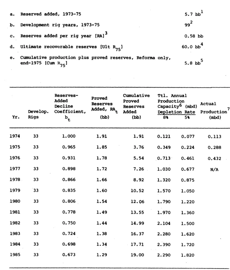
The Reforma results are shown in Table 6. The top part of the table shows the key parameters needed for Equations 5-7; the bottom portion presents the results.' Column 5 shows cumulative reserves added totalling 19 billion barrels (bb) by 1985. Also shown in the table is a forecast of annual production (to be discussed in the following section) which is based on this forecast of reserves-added. The same analysis performed for the rest of Mexico, or for any other nation or sub-national region, will look very much like Table 6.

In this example, an assumed constant rate of development drilling, interacting with government estimates of proved reserves and ultimate recovery, yields a peak production rate of 2.39 million barrels per day

(mbd) reached in 1984, declining thereafter. Yet high-ranking officials forecast a production rate of 7 mbd in the year 2000. This implies considerably larger reserves-added, through more drilling activity, or more effective drilling (reduced rig time per well) than assumed in the model. Note we have assumed a constant number of development rigs. More development drilling would mean proportionately more production, lagged about 3 years. Thus we have identified one or two key variables in Mexico's plan which will change, and to which we must adjust our data set accordingly.

1_{The Mexican authorities use a definition of proved reserves which is}

very close to the strict API concept: "reserves which are expected to be produced by existing wells through primary and secondary recovery;" from Prospectus, Mexico External Bonds Due 1983 (September 1976), p. 17.

Table 6. Sample Calculation of Reserves Added For Reforma Fields, Mexico

a. Reserved added, 1973-75 5.7 bb

b. Development rig years, 1973-75 99

c. Reserves added per rig year [RA] 0.58 bb

d. Ultimate recoverable reserves [Ult R75] 60.0 bb4 e. Cumulative production plus proved reserves, Reforma only,

end-1975 [Cum R751 5.8 bb

Reserves- Cumulative Ttl. Annual

Proved

Added Proved Production

Decline serves Reserves Capacity6 (mbd) Actual Develop. Coefficient, Added, RAt Added Depletion Rate Production7

Yr. Rigs bt (bb) (bb) 8% 5% (mbd) 1974 33 1.000 1.91 1.91 0.121 0.077 0.113 1975 33 0.965 1.85 3.76 0.349 0.224 0.288 1976 33 0.931 1.78 5.54 -0.713 0.461 0.432 1977 33 0.898 1.72 7.26 1.030 0.677 N/A 1978 33 0.866 1.66 8.92 1.320 0.875 1979 33 0.835 1.60 10.52 1.570 1.050 1980 33 0.806 1.54 12.06 1.790 1.220 1981 33 0.778 1.49 13.55 1.970 1.360 1982 33 0.750 1.44 14.99 2.104 1.500 1983 33 0.724 1.38 16.37 2.280 1.620 1984 33 0.698 1.34 17.71 2.'390 1.720 1985 33 0.673 1.29 19.00 2.290 1.820

Notes to Table 6

1. International Petroleum Encyclopedia (IPE), 1976, p. 222.

2. Petroleos Mexicanos, Report of Director General (March 18, 1974 and 1975), Chiapas-Tabasco only. According to Hughes Tool Co. report, there was no substantial increase of rigs in the South Zone from 1974 to 1975. Hence, we assume the same number of development rigs throughout.

3. Line (a) divided by line (b); see Equation 5.

4. Minister of National Patrimony, Francisco Javier Alejo, quoted in El Tiempo, May 17, 1976, and Petroleum Economist, June 1976, as expecting 7 million mbd by 2000 A.D. A linear growth, and assumption of 10 percent depletion rate in 2000 A.D. indicates ultimate added reserves of just over 60 bb.

5. Original Reforma reserves. Differs from line (a) by 100 million barrels already produced.

6. Assumes: (i) a lag structure whereby new proved reserves are fully developed at the following rates: same year (t) 30%, year (t+l) 30%, year (t+2) 40%. This estimation is based on observed lags to full capacity in publicly-reported proved reserves. And (ii) either

(a) 8% depletion annually of pre-existing and of new capacity, which is a weighted average of all large producing Mexico fields excluding Reforma (as calculated from IPE), or (b) 5% depletion annually, which is the announced objective. See IPE, op. cit., p. 191.

7. Reforma fields average production for the first six months of each year (calculated from OGJ). IPE reports total year averages of 0.0 mbd in 1974, 0.274 mbd in 1975, and 0.553 mbd in 1976. The estimates for 1974 and 1975 are probably inaccurate. The Prospectus for Mexican External Bonds,

September 1976, is presumably authoritative, and reports 0.400 mbd

average for the month of December 1975. The 1974 PEMEX: Memoria De Labores, p. 13, reports 0.171 mbd as the total 1974 average with a rate of 0.275 mbd reached in December 1974.

4.2 Analysis of New Capacity and Production Plans

We need now to go from proved reserves-added to attainable new

capacity, as indicated in Figure 3. In some areas we have the companies' own plans. For actual forecasting, they dominate any estimates we could make. Moreover, they are a valuable check on our own calculations, which we make by two possible methods. We may rely again on the inertia of the

system, and base production forecasts on the historical relation of output to proved reserves. We show this method first. Or, it may be possible to analyze the economic forces underlying observed production behavior, and methods of doing that also are discussed below.

But whichever method we use, application of a single depletion rate to a reserve estimate--to obtain a production profile--is a strong

simplification, as Figure 5 shows. In the lower part of the figure, the solid line shows a typical production profile for a field; the area under the curve is the total proved reserves R. The dashed line is our simplified version of oil exploitation where production jumps immediately to an initial (and presumed peak) capacity Qp and declines at a constant percentage rate thereafter. Once again, the area under the curve is R, so that

T -at

R= Q fie dt. (8)

o

As T + a, R + Qp/a; or in the limit, a = Qp/R. The question for analysis then is: what is the value of the depletion rate, a, (and therefore of Qp) that is appropriate for new additions to reserves? Once a is determined it is a simple step to forecasts of supply. The remaining issue is the lag between the time proved reserves are "booked" and the point when the new capacity Qp is on line. In a mature producing

area the lag from the former to the latter is short, but not in a new province. We use, tentatively, 2 years onshore and 4 years offshore,

but in every case including only those fields where development drilling has been started.

4.2.1 Historical Production-Reserve Ratio

As a first approximation, capacity plans can be calculated on the assumption that new additions to proved reserves will be depleted at the

same rate as existing fields. Under the assumption of a uniform policy regarding depletion, the depletion rate for an area can be calculated as

1975

a = E Qt/R7 3-75 (9)

t=1973

where 1973-75 is taken as a reasonable base period for estimation, and R7375 is the average level of proved reserves over that period. Then for any new addition to proved reserves in year t, the new installed capacity is

Qpt = aRt. (10)

Assuming no excess capacity is installed, production from Rt begins at

the level Qt = Qpt and declines at a percent per year.

of course, we need to worry aboutthe degree of error this simplified model may involve. The North Sea affords a check. The end-1973 IPE reserves

(fields under development only) were less than 2 billion barrels. Preliminary indications then (which have, incidentally, been well borne out) were of a 9 percent depletion rate. This would predict 495 tbd in 1977, somewhat over a

year too late, since 1976 and 1977 are now estimated at 585 and 1230 tbd respectively. The end-1975 IPE developed reserves were 9.4 billion barrels, and the same method, again assuming 9 percent, would predict 2.3 mbd in 1979, which seems about on target so far, since late-1976 estimates are for 2.5 mbd

However, the production-reserve ratio for any country is an aggregate of many fields. Hence a simple division of national production by national

reserves may be seriously misleading. A good example is Table 7, showing Abu Dhabi. Total national production was 1.7% of proved-plus-probable

reserves. But the bulk of those "reserves" are still undeveloped; the working inventory is being drawn down much faster. If we confine ourselves

to proved reserves, the simple quotient Q/R = .08 gives equal weight to every barrel of developed reserves. But our true objective is to give equal weight to every barrel produced. If we want to estimate how much Abu Dhabi is capable of producing next year, the Bu Hasa field (156 million barrels) is approximately twice as important as Zakum (82 million).

Accordingly, we weight the production-reserve ratio for each field by its production, and divide the total for all fields by the total weight. This calculation is shown in Table 7. Use of the weighted average mean lets us escape from some of the ill effects of poorly estimated reserves. Since it is a better predictor of future production, it yields more

accurate cost data, which depend on our estimated production profile (Figure 5). We have, of course, a minor sampling problem since we are using the average of the listed fields for the whole country. However, the finite population multiplier is a powerful ally; since we have accounted for 77 percent of the national total of production (394/512), the error cannot be great.

It is likely that outside the United States and Canada, reserves are overstated and therefore decline rates understated. This is not because of errors of optimism, but because undeveloped reservoirs in known fields

Table 7. Weighted Mean Depletion Rate, Abu Dhabi, 1975 (millions of barrels)

Field, Discovery Date

Asab, 1965 Bu Hasa, 1962 Mubarras, 1971 Umm Shaif, 1958 Zakum, 1964 Sub Total Production 90 156 7 59 82 394

Unweighted Mean, total Abu Dhabi: Unweighted Mean, Large Fields: Weighted Mean: ZQ'/ER' = 512/29,500 = 1.7% .Q/TR = 394/4,959 = 8.0% E[Q(Q/R)/EQ = 42.6/394 = 10.8%

Sources: Unweighted Mean, OGJ; others, IPE.

Reserves R 500 1,289 150 1,706 1, 314 4,959 Q2 /R 16.2 18.9 0.3 2.1 5.1 42.6 .180 .121 .047 .035 .062 .080 _ _

Table 8 shows the results of this simple approximation, using the weighted average depletion rate as the decline rate. We have chosen

four widely differing areas to show the meaning of the concepts, and to test two capacity forecasts. The first case is Mexico, which draws on the data used earlier. It is assumed that Antarctica contains 20 billion barrels available but will not be explored or developed. Hence it has, and will have, zero reserves. Abu Dhabi drilling effort, continued at

current levels, leaves them with a 1985 production about where they are now. Iraq attains 4.5 million barrels daily, double current production, but less than the government's announced objective for the year 1980

or 1981.1

4.2.2 Optimal Decline Rate

The value of a observed in historical data, and calculated by Equation 9, is the result of a particular set of past conditions of

cost, price, and tax. It may or may not be an appropriate guide to future behavior under different conditions, and therefore we should like to be able to calculate this parameter. We can do this by assuming profit-maximizing behavior on the part of oil operators, and solving

for the optimal depletion rate, a*, based on estimates of cost per barrel and future price.

First, it is assumed that the profile of capital expenditures E_t shown in Figure 5 can be collapsed to a single-period outlay I. Data on operating costs are rather sketchy; fortunately the bulk of costs

The equating of capacity with production assumes that these cartel nations are not forced to hold excess capacity in order to help support the price.

O0D 0 0) o N 0 LA 00 oH ,-4 Ln ODH I d 0 H a 0 4 U)

v-

4JO

0I

· 4 > 0 '0 .. )4

ao

la

H

44

H Q N 0 g o :3 r4 H 0 Q) . c t I N Xe *.

Ot

.9- 4 UP4 it 4.1 0 0 u

0

o n IT o L ko

o

0

H

19 0 Ln 0 '.0 0 LA NV H

o

o

0

0

0 H Un H H H

o

0

0

0

o

o

O o

' N r-* * H H

a

Oa N 0 C4 CV 0 A

I

N

O 0N 0 H4

0 0

> C 44 0O-_ 'U .9-4 4-, 4.) .14

I

8

Hy, H LI CD I u3 .- 4 a o C) Cl a4

0

0 U_k 0 4.0-4 U) 0 rn cu (A -a) N N Id R 44 o U) -4 A,_R -p .H, 0 4-) 0 4 _o

4

e4 0 .,-4 4-) ,-4₀ .9a a4J 'U >-4 Fe 0 H 04 0 0 r 4

0 0

U) 440 0 t 4 w_o ·O 0 N 0 P4 0 _O0 H WnW 4-1_U) 0 04 C) ₀

_~k

a

o

_{0 i} O-H_{N 0} O V r,1 U) N X H H . _{O f XE}U AO t u * Q) k 0 He 4-x 0 .,-I .el .rq 0 u a₀ N, >1 0 a) 0 0 U) .H 9-4 + (A 0 N *,l₀ .4' En En U) 0 0 U/) -