Publisher’s version / Version de l'éditeur: Computer Science, 2017-08-11
READ THESE TERMS AND CONDITIONS CAREFULLY BEFORE USING THIS WEBSITE. https://nrc-publications.canada.ca/eng/copyright
Vous avez des questions? Nous pouvons vous aider. Pour communiquer directement avec un auteur, consultez la première page de la revue dans laquelle son article a été publié afin de trouver ses coordonnées. Si vous n’arrivez pas à les repérer, communiquez avec nous à [email protected].
Questions? Contact the NRC Publications Archive team at
[email protected]. If you wish to email the authors directly, please see the first page of the publication for their contact information.
NRC Publications Archive
Archives des publications du CNRC
This publication could be one of several versions: author’s original, accepted manuscript or the publisher’s version. / La version de cette publication peut être l’une des suivantes : la version prépublication de l’auteur, la version acceptée du manuscrit ou la version de l’éditeur.
Access and use of this website and the material on it are subject to the Terms and Conditions set forth at
WASSA-2017 shared task on emotion intensity
Mohammad, Saif M.; Bravo-Marquez, Felipe
https://publications-cnrc.canada.ca/fra/droits
L’accès à ce site Web et l’utilisation de son contenu sont assujettis aux conditions présentées dans le site LISEZ CES CONDITIONS ATTENTIVEMENT AVANT D’UTILISER CE SITE WEB.
NRC Publications Record / Notice d'Archives des publications de CNRC: https://nrc-publications.canada.ca/eng/view/object/?id=4230a39d-5839-4465-9212-8cb2163b9037 https://publications-cnrc.canada.ca/fra/voir/objet/?id=4230a39d-5839-4465-9212-8cb2163b9037
See discussions, stats, and author profiles for this publication at: https://www.researchgate.net/publication/319121494
WASSA-2017 Shared Task on Emotion Intensity
Article · August 2017 CITATIONS0
READS11
2 authors: Some of the authors of this publication are also working on these related projects: AffectiveTweetsView project Saif Mohammad National Research Council Canada 80 PUBLICATIONS 2,239 CITATIONS SEE PROFILE Felipe Bravo-Marquez The University of Waikato 22 PUBLICATIONS 199 CITATIONS SEE PROFILE All content following this page was uploaded by Felipe Bravo-Marquez on 22 August 2017. The user has requested enhancement of the downloaded file.
WASSA-2017 Shared Task on Emotion Intensity
Saif M. Mohammad
Information and Communications Technologies National Research Council Canada
Ottawa, Canada
Felipe Bravo-Marquez Department of Computer Science
The University of Waikato Hamilton, New Zealand
Abstract
We present the first shared task on de-tecting the intensity of emotion felt by the speaker of a tweet. We create the first datasets of tweets annotated for anger, fear, joy, and sadness intensities using a technique called best–worst scal-ing (BWS). We show that the annota-tions lead to reliable fine-grained intensity scores (rankings of tweets by intensity). The data was partitioned into training, de-velopment, and test sets for the compe-tition. Twenty-two teams participated in the shared task, with the best system ob-taining a Pearson correlation of 0.747 with the gold intensity scores. We summarize the machine learning setups, resources, and tools used by the participating teams, with a focus on the techniques and re-sources that are particularly useful for the task. The emotion intensity dataset and the shared task are helping improve our under-standing of how we convey more or less intense emotions through language. 1 Introduction
We use language to communicate not only the emotion we are feeling but also the intensity of the emotion. For example, our utterances can con-vey that we are very angry, slightly sad, absolutely elated, etc. Here, intensity refers to the degree or amount of an emotion such as anger or sadness.1 Automatically determining the intensity of emo-tion felt by the speaker has applicaemo-tions in com-merce, public health, intelligence gathering, and social welfare.
1
Intensity should not be confused with arousal, which refers to activation–deactivation dimension—the extent to which an emotion is calming or exciting.
Twitter has a large and diverse user base which entails rich textual content, including non-standard language such as emoticons, emojis, cre-atively spelled words (happee), and hashtagged words (#luvumom). Tweets are often used to con-vey one’s emotion, opinion, and stance ( Moham-mad et al., 2017). Thus, automatically detecting emotion intensities in tweets is especially bene-ficial in applications such as tracking brand and product perception, tracking support for issues and policies, tracking public health and well-being, and disaster/crisis management. Here, for the first time, we present a shared task on automatically detecting intensity of emotion felt by the speaker of a tweet: WASSA-2017 Shared Task on Emotion Intensity.2
Specifically, given a tweet and an emotion X, the goal is to determine the intensity or degree of emotion X felt by the speaker—a real-valued score between 0 and 1.3 A score of 1 means that the speaker feels the highest amount of emotion X. A score of 0 means that the speaker feels the low-est amount of emotion X. We first ask human an-notators to infer this intensity of emotion from a tweet. Later, automatic algorithms are tested to determine the extent to which they can replicate human annotations. Note that often a tweet does not explicitly state that the speaker is experienc-ing a particular emotion, but the intensity of emo-tion felt by the speaker can be inferred nonethe-less. Sometimes a tweet is sarcastic or it conveys the emotions of a different entity, yet the annota-tors (and automatic algorithms) are to infer, based on the tweet, the extent to which the speaker is likely feeling a particular emotion.
2
http://saifmohammad.com/WebPages/EmotionIntensity-SharedTask.html
3
Identifying intensity of emotion evoked in the reader, or intensity of emotion felt by an entity mentioned in the tweet, are also useful tasks, and left for future work.
In order to provide labeled training, develop-ment, and test sets for this shared task, we needed to annotate instances for degree of affect. This is a substantially more difficult undertaking than an-notating only for the broad affect class: respon-dents are presented with greater cognitive load and it is particularly hard to ensure consistency (both across responses by different annotators and within the responses produced by an individual an-notator). Thus, we used a technique called Best–
Worst Scaling (BWS), also sometimes referred to as Maximum Difference Scaling (MaxDiff). It is an annotation scheme that addresses the limita-tions of traditional rating scales (Louviere,1991;
Louviere et al., 2015; Kiritchenko and Moham-mad, 2016, 2017). We used BWS to create the
Tweet Emotion Intensity Dataset, which currently includes four sets of tweets annotated for inten-sity of anger, fear, joy, and sadness, respectively (Mohammad and Bravo-Marquez, 2017). These are the first datasets of their kind.
The competition is organized on a CodaLab website, where participants can upload their sub-missions, and the leaderboard reports the results.4 Twenty-two teams participated in the 2017 it-eration of the competition. The best perform-ing system, Prayas, obtained a Pearson correla-tion of 0.747 with the gold annotacorrela-tions. Seven teams obtained scores higher than the score ob-tained by a competitive SVM-based benchmark system (0.66), which we had released at the start of the competition.5 Low-dimensional (dense) distributed representations of words (word em-beddings) and sentences (sentence vectors), along with presence of affect–associated words (derived from affect lexicons) were the most commonly used features. Neural network were the most com-monly used machine learning architecture. They were used for learning tweet representations as well as for fitting regression functions. Support vector machines (SVMs) were the second most popular regression algorithm. Keras and Tensor-Flow were some of the most widely used libraries. The top performing systems used ensembles of models trained on dense distributed representa-tions of the tweets as well as features drawn from affect lexicons. They also made use of a substan-tially larger number of affect lexicons than sys-tems that did not perform as well.
4
https://competitions.codalab.org/competitions/16380
5
https://github.com/felipebravom/AffectiveTweets
The emotion intensity dataset and the corre-sponding shared task are helping improve our un-derstanding of how we convey more or less in-tense emotions through language. The task also adds a dimensional nature to model of basic emo-tions, which has traditionally been viewed as cat-egorical (joy or no joy, fear or no fear, etc.). On going work with annotations on the same data for valence , arousal, and dominance aims to bet-ter understand the relationships between the cir-cumplex model of emotions (Russell, 2003) and the categorical model of emotions (Ekman,1992;
Plutchik, 1980). Even though the 2017 WASSA shared task has concluded, the CodaLab competi-tion website is kept open. Thus new and improved systems can continually be tested. The best results obtained by any system on the 2017 test set can be found on the CodaLab leaderboard.
The rest of the paper is organized as follows. We begin with related work and a brief back-ground on best–worst scaling (Section 2). In Sec-tion 3, we describe how we collected and anno-tated the tweets for emotion intensity. We also present experiments to determine the quality of the annotations. Section 4 presents details of the shared task setup. In Section 5, we present a com-petitive SVM-based baseline that uses a number of common text classification features. We describe ablation experiments to determine the impact of different feature types on regression performance. In Section 6, we present the results obtained by the participating systems and summarize their ma-chine learning setups. Finally, we present conclu-sions and future directions. All of the data, annota-tion quesannota-tionnaires, evaluaannota-tion scripts, regression code, and interactive visualizations of the data are made freely available on the shared task website.2
2 Related Work 2.1 Emotion Annotation
Psychologists have argued that some emotions are more basic than others (Ekman, 1992; Plutchik,
1980;Parrot,2001;Frijda, 1988). However, they disagree on which emotions (and how many) should be classified as basic emotions—some pro-pose 6, some 8, some 20, and so on. Thus, most ef-forts in automatic emotion detection have focused on a handful of emotions, especially since manu-ally annotating text for a large number of emotions is arduous. Apart from these categorical models of emotions, certain dimensional models of emotion
have also been proposed. The most popular among them, Russell’s circumplex model, asserts that all emotions are made up of two core dimensions: valence and arousal (Russell, 2003). We created datasets for four emotions that are the most com-mon acom-mongst the many proposals for basic emo-tions: anger, fear, joy, and sadness. However, we have also begun work on other affect categories, as well as on valence and arousal.
The vast majority of emotion annotation work provides discrete binary labels to the text instances (joy–nojoy, fear–nofear, and so on) (Alm et al.,
2005;Aman and Szpakowicz,2007;Brooks et al.,
2013; Neviarouskaya et al., 2009; Bollen et al.,
2009). The only annotation effort that provided scores for degree of emotion is byStrapparava and Mihalcea (2007) as part of one of the SemEval-2007 shared task. Annotators were given newspa-per headlines and asked to provide scores between 0 and 100 via slide bars in a web interface. It is dif-ficult for humans to provide direct scores at such fine granularity. A common problem is inconsis-tency in annotations. One annotator might assign a score of 79 to a piece of text, whereas another an-notator may assign a score of 62 to the same text. It is also common that the same annotator assigns different scores to the same text instance at differ-ent points in time. Further, annotators often have a bias towards different parts of the scale, known as scale region bias.
2.2 Best–Worst Scaling
Best–Worst Scaling (BWS)was developed by Lou-viere (1991), building on some ground-breaking research in the 1960s in mathematical psychology and psychophysics by Anthony A. J. Marley and Duncan Luce. Annotators are given n items (an n-tuple, where n > 1 and commonly n = 4). They are asked which item is the best (highest in terms of the property of interest) and which is the worst (lowest in terms of the property of interest). When working on 4-tuples, best–worst annotations are particularly efficient because each best and worst annotation will reveal the order of five of the six item pairs. For example, for a 4-tuple with items A, B, C, and D, if A is the best, and D is the worst, then A > B, A > C, A > D, B > D, and C > D.
BWS annotations for a set of 4-tuples can be easily converted into real-valued scores of associ-ation between the items and the property of inter-est (Orme,2009;Flynn and Marley,2014). It has
Emotion Thes. Category Head Word anger 900 resentment
fear 860 fear
joy 836 cheerfulness sadness 837 dejection
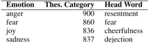
Table 1: Categories from the Roget’s Thesaurus whose words were taken to be the query terms.
been empirically shown that annotations for 2N 4-tuples is sufficient for obtaining reliable scores (where N is the number of items) (Louviere,1991;
Kiritchenko and Mohammad,2016).6
Kiritchenko and Mohammad (2017) show through empirical experiments that BWS produces more reliable fine-grained scores than scores ob-tained using rating scales. Within the NLP com-munity, Best–Worst Scaling (BWS) has thus far been used only to annotate words: for exam-ple, for creating datasets for relational similar-ity (Jurgens et al.,2012), word-sense disambigua-tion (Jurgens, 2013), word–sentiment intensity (Kiritchenko et al., 2014), and phrase sentiment composition (Kiritchenko and Mohammad,2016). However, we use BWS to annotate whole tweets for intensity of emotion.
3 Data
Mohammad and Bravo-Marquez (2017) describe how the Tweet Emotion Intensity Dataset was cre-ated. We summarize below the approach used and the key properties of the dataset. Not in-cluded in this summary are: (a) experiments show-ing marked similarities between emotion pairs in terms of how they manifest in language, (b) how training data for one emotion can be used to im-prove prediction performance for a different emo-tion, and (c) an analysis of the impact of hashtag words on emotion intensities.
For each emotion X, we select 50 to 100 terms that are associated with that emotion at differ-ent intensity levels. For example, for the anger dataset, we use the terms: angry, mad, frustrated,
annoyed, peeved, irritated, miffed, fury, antago-nism,and so on. For the sadness dataset, we use the terms: sad, devastated, sullen, down, crying,
dejected, heartbroken, grief, weeping, and so on. We will refer to these terms as the query terms.
We identified the query words for an emotion 6
At its limit, when n = 2, BWS becomes a paired
com-parison (Thurstone, 1927;David, 1963), but then a much larger set of tuples need to be annotated (closer to N2).
by first searching the Roget’s Thesaurus to find categories that had the focus emotion word (or a close synonym) as the head word.7 The categories chosen for each head word are shown in Table
1. We chose all single-word entries listed within these categories to be the query terms for the cor-responding focus emotion.8 Starting November 22, 2016, and continuing for three weeks, we polled the Twitter API for tweets that included the query terms. We discarded retweets (tweets that start with RT) and tweets with urls. We created a subset of the remaining tweets by:
• selecting at most 50 tweets per query term. • selecting at most 1 tweet for every tweeter–
query term combination.
Thus, the master set of tweets is not heavily skewed towards some tweeters or query terms.
To study the impact of emotion word hashtags on the intensity of the whole tweet, we identified tweets that had a query term in hashtag form towards the end of the tweet—specifically, within the trailing portion of the tweet made up solely of hashtagged words. We created copies of these tweets and then removed the hashtag query terms from the copies. The updated tweets were then added to the master set. Finally, our master set of 7,097 tweets includes:
1. Hashtag Query Term Tweets (HQT Tweets): 1030 tweets with a query term in the form of a hashtag (#<query term>) in the trailing portion of the tweet;
2. No Query Term Tweets (NQT Tweets):
1030 tweets that are copies of ‘1’, but with the hashtagged query term removed;
3. Query Term Tweets (QT Tweets): 5037 tweets that include:
a. tweets that contain a query term in the form of a word (no #<query term>)
b. tweets with a query term in hashtag form followed by at least one non-hashtag word. The master set of tweets was then manually an-notated for intensity of emotion. Table3shows a breakdown by emotion.
7
The Roget’s Thesaurus groups words into about 1000 categories, each containing on average about 100 closely re-lated words. The head word is the word that best represents the meaning of the words within that category.
8
The full list of query terms is available on request.
3.1 Annotating with Best–Worst Scaling We followed the procedure described in Kir-itchenko and Mohammad (2016) to obtain BWS annotations. For each emotion, the annotators were presented with four tweets at a time (4-tuples) and asked to select the speakers of the tweets with the highest and lowest emotion inten-sity. 2 × N (where N is the number of tweets in the emotion set) distinct 4-tuples were ran-domly generated in such a manner that each item is seen in eight different 4-tuples, and no pair of items occurs in more than one 4-tuple. We re-fer to this as random maximum-diversity selection
(RMDS). RMDS maximizes the number of unique items that each item co-occurs with in the 4-tuples. After BWS annotations, this in turn leads to di-rect comparative ranking information for the max-imum number of pairs of items.9
It is desirable for an item to occur in sets of 4-tuples such that the the maximum intensities in those 4-tuples are spread across the range from low intensity to high intensity, as then the propor-tion of times an item is chosen as the best is indica-tive of its intensity score. Similarly, it is desirable for an item to occur in sets of 4-tuples such that the minimum intensities are spread from low to high intensity. However, since the intensities of items are not known before the annotations, RMDS is used.
Every 4-tuple was annotated by three indepen-dent annotators.10 The questionnaires used were developed through internal discussions and pilot annotations. (See the Appendix (8.1) for a sample questionnaire. All questionnaires are also avail-able on the task website.)
The 4-tuples of tweets were uploaded on the crowdsourcing platform, CrowdFlower. About 5% of the data was annotated internally before-hand (by the authors). These questions are referred to as gold questions. The gold questions are inter-spersed with other questions. If one gets a gold 9In combinatorial mathematics, balanced incomplete
block designrefers to creating blocks (or tuples) of a handful items from a set of N items such that each item occurs in the same number of blocks (say x) and each pair of distinct items occurs in the same number of blocks (say y), where x and y are integers ge 1 (Yates,1936). The set of tuples we create have similar properties, except that since we create only 2N tuples, pairs of distinct items either never occur together in a 4-tuple or they occur in exactly one 4-tuple.
10Kiritchenko and Mohammad(2016) showed that using
just three annotations per 4-tuple produces highly reliable re-sults. Note that since each tweet is seen in eight different 4-tuples, we obtain 8 × 3 = 24 judgments over each tweet.
question wrong, they are immediately notified of it. If one’s accuracy on the gold questions falls be-low 70%, they are refused further annotation, and all of their annotations are discarded. This serves as a mechanism to avoid malicious annotations.11
The BWS responses were translated into scores by a simple calculation (Orme, 2009; Flynn and Marley, 2014): For each item t, the score is the percentage of times the t was chosen as having the most intensity minus the percentage of times t was chosen as having the least intensity.12
intensity(t) = %most(t) − %least(t) (1) Since intensity of emotion is a unipolar scale, we linearly transformed the the −100 to 100 scores to scores in the range 0 to 1.
3.2 Reliability of Annotations
A useful measure of quality is reproducibility of the end result—if repeated independent manual annotations from multiple respondents result in similar intensity rankings (and scores), then one can be confident that the scores capture the true emotion intensities. To assess this reproducibility, we calculate average split-half reliability (SHR), a commonly used approach to determine consis-tency (Kuder and Richardson, 1937; Cronbach,
1946). The intuition behind SHR is as follows. All annotations for an item (in our case, tuples) are randomly split into two halves. Two sets of scores are produced independently from the two halves. Then the correlation between the two sets of scores is calculated. If the annotations are of good quality, then the correlation between the two halves will be high.
Since each tuple in this dataset was annotated by three annotators (odd number), we calculate SHR by randomly placing one or two annotations per tuple in one bin and the remaining (two or one) annotations for the tuple in another bin. Then two sets of intensity scores (and rankings) are calcu-lated from the annotations in each of the two bins. 11In case more than one item can be reasonably chosen as
the best (or worst) item, then more than one acceptable gold answers are provided. The goal with the gold annotations is to identify clearly poor or malicious annotators. In case where two items are close in intensity, we want the crowd of annotators to indicate, through their BWS annotations, the relative ranking of the items.
12Kiritchenko and Mohammad (2016) provide code
for generating tuples from items using RMDS, as well as code for generating scores from BWS annotations: http://saifmohammad.com/WebPages/BestWorst.html
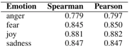
Emotion Spearman Pearson anger 0.779 0.797 fear 0.845 0.850 joy 0.881 0.882 sadness 0.847 0.847
Table 2: Split-half reliabilities (as measured by Pearson correlation and Spearman rank correla-tion) for the anger, fear, joy, and sadness tweets in the Tweet Emotion Intensity Dataset.
The process is repeated 100 times and the correla-tions across the two sets of rankings and intensity scores are averaged. Table2shows the split-half reliabilities for the anger, fear, joy, and sadness tweets in the Tweet Emotion Intensity Dataset.13 Observe that for fear, joy, and sadness datasets, both the Pearson correlations and the Spearman rank correlations lie between 0.84 and 0.88, indi-cating a high degree of reproducibility. However, the correlations are slightly lower for anger indi-cating that it is relative more difficult to ascertain the degrees of anger of speakers from their tweets. Note that SHR indicates the quality of annotations obtained when using only half the number of an-notations. The correlations obtained when repeat-ing the experiment with three annotations for each 4-tuple is expected to be even higher. Thus the numbers shown in Table 2are a lower bound on the quality of annotations obtained with three an-notations per 4-tuple.
4 Task Setup 4.1 The Task
Given a tweet and an emotion X, automatic sys-tems have to determine the intensity or degree of emotion X felt by the speaker—a real-valued score between 0 and 1. A score of 1 means that the speaker feels the highest amount of emotion X. A score of 0 means that the speaker feels the low-est amount of emotion X. The competition is or-ganized on a CodaLab website, where participants can upload their submissions, and the leaderboard reports the results.14
13
Past work has found the SHR for sentiment intensity an-notations for words, with 8 anan-notations per tuple, to be 0.98 (Kiritchenko et al.,2014). In contrast, here SHR is calculated from 3 annotations, for emotions, and from whole sentences. SHR determined from a smaller number of annotations and on more complex annotation tasks are expected to be lower.
14
Emotion Train Dev. Test All anger 857 84 760 1701 fear 1147 110 995 2252 joy 823 74 714 1611 sadness 786 74 673 1533 All 3613 342 3142 7097
Table 3: The number of instances in the Tweet Emotion Intensity dataset.
4.2 Training, development, and test sets The Tweet Emotion Intensity Dataset is partitioned into training, development, and test sets for ma-chine learning experiments (see Table3). For each emotion, we chose to include about 50% of the tweets in the training set, about 5% in the develop-ment set, and about 45% in the test set. Further, we ensured that an No-Query-Term (NQT) tweet is in the same partition as the Hashtag-Query-Term (HQT) tweet it was created from.
The training and development sets were made available more than two months before the two-week official evaluation period. Participants were told that the development set could be used to tune ones system and also to test making a submission on CodaLab. Gold intensity scores for the devel-opment set were released two weeks before the evaluation period, and participants were free to train their systems on the combined training and development sets, and apply this model to the test set. The test set was released at the start of the evaluation period.
4.3 Resources
Participants were free to use lists of manu-ally created and/or automaticmanu-ally generated word– emotion and word–sentiment association lexi-cons.15 Participants were free to build a system from scratch or use any available software pack-ages and resources, as long as they are not against the spirit of fair competition. In order to assist testing of ideas, we also provided a baseline Weka system for determining emotion intensity, that par-ticipants can build on directly or use to determine the usefulness of different features.16We describe the baseline system in the next section.
15
A large number of sentiment and emo-tion lexicons created at NRC are available here: http://saifmohammad.com/WebPages/lexicons.html
16
https://github.com/felipebravom/AffectiveTweets
4.4 Official Submission to the Shared Task System submissions were required to have the same format as used in the training and test sets. Each line in the file should include:
id[tab]tweet[tab]emotion[tab]score Each team was allowed to make as many as ten submissions during the evaluation period. How-ever, they were told in advance that only the fi-nal submission would be considered as the official submission to the competition.
Once the evaluation period concluded, we re-leased the gold labels and participants were able to determine results on various system variants that they may have developed. We encouraged par-ticipants to report results on all of their systems (or system variants) in the system-description pa-per that they write. However, they were asked to clearly indicate the result of their official submis-sion.
During the evaluation period, the CodaLab leaderboard was hidden from participants—so they were unable see the results of their submis-sions on the test set until the leaderboard was sub-sequently made public. Participants were, how-ever, able to immediately see any warnings or er-rors that their submission may have triggered. 4.5 Evaluation
For each emotion, systems were evaluated by cal-culating the Pearson Correlation Coefficient of the system predictions with the gold ratings. Pearson coefficient, which measures linear correlations be-tween two variables, produces scores from -1 (per-fectly inversely correlated) to 1 (per(per-fectly corre-lated). A score of 0 indicates no correlation. The correlation scores across all four emotions was av-eraged to determine the bottom-line competition metric by which the submissions were ranked.
In addition to the bottom-line competition ric described above, the following additional met-rics were also provided:
• Spearman Rank Coefficient of the submission with the gold scores of the test data.
Motivation: Spearman Rank Coefficient consid-ers only how similar the two sets of ranking are. The differences in scores between adja-cently ranked instance pairs is ignored. On the one hand this has been argued to alleviate some biases in Pearson, but on the other hand it can ignore relevant information.
• Correlation scores (Pearson and Spearman) over a subset of the testset formed by taking in-stances with gold intensity scores ≥0.5. Motivation: In some applications, only those instances that are moderately or strongly emo-tional are relevant. Here it may be much more important for a system to correctly determine emotion intensities of instances in the higher range of the scale as compared to correctly de-termine emotion intensities in the lower range of the scale.
Results with Spearman rank coefficient were largely inline with those obtained using Pearson coefficient, and so in the rest of the paper we report only the latter. However, the CodaLab leaderboard and the official results posted on the task website show both metrics. The official evaluation script (which calculates correlations using both metrics and also acts as a format checker) was made avail-able along with the training and development data well in advance. Participants were able to use it to monitor progress of their system by cross-validation on the training set or testing on the de-velopment set. The script was also uploaded on the CodaLab competition website so that the sys-tem evaluates submissions automatically and up-dates the leaderboard.
5 Baseline System for Automatically Determining Tweet Emotion Intensity 5.1 System
We implemented a package called Affec-tiveTweets (Mohammad and Bravo-Marquez,
2017) for the Weka machine learning workbench (Hall et al., 2009). It provides a collection of filters for extracting features from tweets for sentiment classification and other related tasks. These include features used inKiritchenko et al.
(2014) and Mohammad et al. (2017).17 We use the AffectiveTweets package for calculating fea-ture vectors from our emotion-intensity-labeled tweets and train Weka regression models on this transformed data. The regression model used is an L2-regularized L2-loss SVM regression model with the regularization parameter C set to 1, 17Kiritchenko et al. (2014) describes the NRC-Canada
system which ranked first in three sentiment shared tasks: 2013 Task 2, 2014 Task 9, and SemEval-2014 Task 4. Mohammad et al.(2017) describes a stance-detection system that outperformed submissions from all 19 teams that participated in SemEval-2016 Task 6.
implemented in LIBLINEAR18. The system uses the following features:19
a. Word N-grams (WN): presence or absence of word n-grams from n= 1 to n = 4.
b. Character N-grams (CN): presence or absence of character n-grams from n= 3 to n = 5.
c. Word Embeddings (WE): an average of the word embeddings of all the words in a tweet. We calculate individual word embeddings using the negative sampling skip-gram model implemented in Word2Vec (Mikolov et al.,2013). Word vectors are trained from ten million English tweets taken from the Edinburgh Twitter Corpus (Petrovi´c et al., 2010). We set Word2Vec parameters: window size: 5; number of dimensions: 400.20
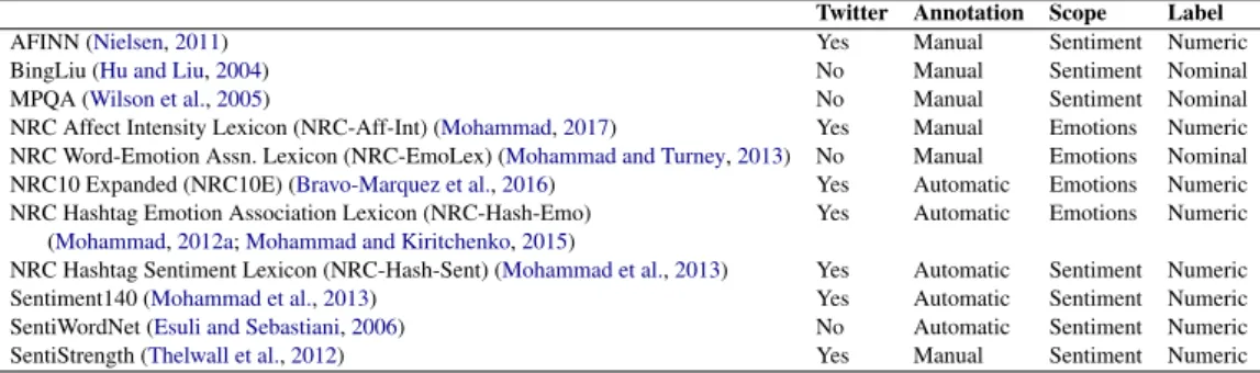
d. Affect Lexicons (L): we use the lexicons shown in Table 4by aggregating the information for all the words in a tweet. If the lexicon provides nom-inal association labels (e.g, positive, anger, etc.), then the number of words in the tweet matching each class are counted. If the lexicon provides nu-merical scores, the individual scores for each class are summed. and whether the affective associa-tions provided are nominal or numeric.
5.2 Experiments
We developed the baseline system by learning models from each of the Tweet Emotion Intensity
Datasettraining sets and applying them to the cor-responding development sets. Once the system parameters were frozen, the system learned new models from the combined training and develop-ment corpora. This model was applied to the test sets. Table 5 shows the results obtained on the test sets using various features, individually and in combination. The last column ‘avg.’ shows the macro-average of the correlations for all of the emotions.
Using just character or just word n-grams leads to results around 0.48, suggesting that they are rea-sonably good indicators of emotion intensity by themselves. (Guessing the intensity scores at ran-dom between 0 and 1 is expected to get correla-tions close to 0.) Word embeddings produces sta-tistically significant improvement over the ngrams (avg. r = 0.55).21 Using features drawn from
af-18
http://www.csie.ntu.edu.tw/∼cjlin/liblinear/
19See Appendix (A.3) for further implementation details. 20
Optimized for the task of word–emotion classification on an independent dataset (Bravo-Marquez et al.,2016).
21
We used the Wilcoxon signed-rank test at 0.05 signifi-cance level calculated from ten random partitions of the data, for all the significance tests reported in this paper.
Twitter Annotation Scope Label AFINN (Nielsen,2011) Yes Manual Sentiment Numeric BingLiu (Hu and Liu,2004) No Manual Sentiment Nominal MPQA (Wilson et al.,2005) No Manual Sentiment Nominal NRC Affect Intensity Lexicon (NRC-Aff-Int) (Mohammad,2017) Yes Manual Emotions Numeric NRC Word-Emotion Assn. Lexicon (NRC-EmoLex) (Mohammad and Turney,2013) No Manual Emotions Nominal NRC10 Expanded (NRC10E) (Bravo-Marquez et al.,2016) Yes Automatic Emotions Numeric NRC Hashtag Emotion Association Lexicon (NRC-Hash-Emo) Yes Automatic Emotions Numeric
(Mohammad,2012a;Mohammad and Kiritchenko,2015)
NRC Hashtag Sentiment Lexicon (NRC-Hash-Sent) (Mohammad et al.,2013) Yes Automatic Sentiment Numeric Sentiment140 (Mohammad et al.,2013) Yes Automatic Sentiment Numeric SentiWordNet (Esuli and Sebastiani,2006) No Automatic Sentiment Numeric SentiStrength (Thelwall et al.,2012) Yes Manual Sentiment Numeric
Table 4: Affect lexicons used in our experiments.
fect lexicons produces results ranging from avg. r = 0.19 with SentiWordNet to avg. r = 0.53 with NRC-Hash-Emo. Combining all the lexicons leads to statistically significant improvement over individual lexicons (avg. r = 0.63). Combining the different kinds of features leads to even higher scores, with the best overall result obtained us-ing word embeddus-ing and lexicon features (avg. r = 0.66).22 The feature space formed by all the lexicons together is the strongest single feature category. The results also show that some fea-tures such as character ngrams are redundant in the presence of certain other features.
Among the lexicons, NRC-Hash-Emo is the most predictive single lexicon. Lexicons that clude Twitter-specific entries, lexicons that in-clude intensity scores, and lexicons that label emotions and not just sentiment, tend to be more predictive on this task–dataset combination. NRC-Aff-Int has real-valued fine-grained word– emotion association scores for all the words in NRC-EmoLex that were marked as being associ-ated with anger, fear, joy, and sadness.23 Improve-ment in scores obtained using NRC-Aff-Int over the scores obtained using NRC-EmoLex also show that using fine intensity scores of word-emotion association are beneficial for tweet-level emotion intensity detection. The correlations for anger, fear, and joy are similar (around 0.65), but the cor-relation for sadness is markedly higher (0.71). We can observe from Table5that this boost in perfor-mance for sadness is to some extent due to word embeddings, but is more so due to lexicon fea-tures, especially those from SentiStrength. Sen-tiStrength focuses solely on positive and negative classes, but provides numeric scores for each.
To assess performance in the moderate-to-high range of the intensity scale, we calculated
correla-22
The increase from 0.63 to 0.66 is statistically significant.
23
http://saifmohammad.com/WebPages/AffectIntensity.htm
Pearson correlation r anger fear joy sad. avg.
Individual feature sets
word ngrams (WN) 0.42 0.49 0.52 0.49 0.48 char. ngrams (CN) 0.50 0.48 0.45 0.49 0.48 word embeds. (WE) 0.48 0.54 0.57 0.60 0.55 all lexicons (L) 0.62 0.60 0.60 0.68 0.63 Individual Lexicons AFINN 0.48 0.27 0.40 0.28 0.36 BingLiu 0.33 0.31 0.37 0.23 0.31 MPQA 0.18 0.20 0.28 0.12 0.20 NRC-Aff-Int 0.24 0.28 0.37 0.32 0.30 NRC-EmoLex 0.18 0.26 0.36 0.23 0.26 NRC10E 0.35 0.34 0.43 0.37 0.37 NRC-Hash-Emo 0.55 0.55 0.46 0.54 0.53 NRC-Hash-Sent 0.33 0.24 0.41 0.39 0.34 Sentiment140 0.33 0.41 0.40 0.48 0.41 SentiWordNet 0.14 0.19 0.26 0.16 0.19 SentiStrength 0.43 0.34 0.46 0.61 0.46 Combinations WN + CN + WE 0.50 0.48 0.45 0.49 0.48 WN + CN + L 0.61 0.61 0.61 0.63 0.61 WE + L 0.64 0.63 0.65 0.71 0.66 WN + WE + L 0.63 0.65 0.65 0.65 0.65 CN + WE + L 0.61 0.61 0.62 0.63 0.62 WN + CN + WE + L 0.61 0.61 0.61 0.63 0.62
Over the subset of test set where intensity ≥0.5
WN + WE + L 0.51 0.51 0.40 0.49 0.47 Table 5: Pearson correlations (r) of emotion inten-sity predictions with gold scores. Best results for each column are shown in bold: highest score by a feature set, highest score using a single lexicon, and highest score using feature set combinations.
tion scores over a subset of the test data formed by taking only those instances with gold emotion in-tensity scores ≥0.5. The last row in Table5shows the results. We observe that the correlation scores are in general lower here in the 0.5 to 1 range of intensity scores than in the experiments over the full intensity range. This is simply because this is a harder task as now the systems do not benefit by making coarse distinctions over whether a tweet is in the lower range or in the higher range.
6 Official System Submissions to the Shared Task
Twenty-two teams made submissions to the shared task. In the subsections below we present the re-sults and summarize the approaches and resources used by the participating systems.
6.1 Results
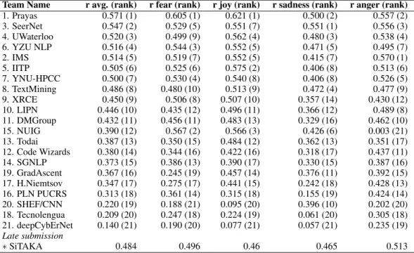
Table 6 shows the Pearson correlations (r) and ranks (in brackets) obtained by the systems on the full test sets. The bottom-line competition met-ric, ‘r avg.’, is the average of Pearson correlations obtained for each of the four emotions. (The task website shows Spearman rank coefficient as well. Those scores are close in value to the Pearson cor-relations, and most teams rank the same by either metric.) The top ranking system, Prayas, obtained an r avg. of 0.747. It obtains slightly better cor-relations for joy and anger (around 0.76) than for fear and sadness (around 0.73). IMS, which ranked second overall, obtained slightly higher correla-tion on anger, but lower scores than Prayas on the other emotions. The top 12 teams all obtain their best correlation on anger as opposed to any of the other three emotions. They obtain lowest correla-tions on fear and sadness. Seven teams obtained scores higher than that obtained by the publicly available benchmark system (r avg. = 0.66).
Table 7shows the Pearson correlations (r) and ranks (in brackets) obtained by the systems on those instances in the test set with intensity scores ≥ 0.5. Prayas obtains the best results here too with r avg. = 0.571. SeerNet, which ranked third on the full test set, ranks second on this subset. As found in the baseline results, system results on this subset overall are lower than than on the full test set. Most systems perform best on the joy data and worst on the sadness data.
6.2 Machine Learning Setups
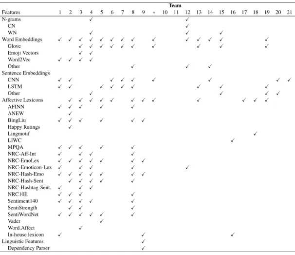
Systems followed a supervised learning approach in which tweets were mapped into feature vectors that were then used for training regression models. Features were drawn both from the training data as well as from external resources such as large tweet corpora and affect lexicons. Table
8 lists the feature types (resources) used by the teams. (To save space, team names are abbre-viated to just their rank on the full test set (as shown in Table 6).) Commonly used features included word embeddings and sentence
repre-sentations learned using neural networks (sen-tence embeddings). Some of the word embed-dings models used were Glove (SeerNet, UWa-terloo, YZU NLP), Word2Vec (SeerNet), and Word Vector Emoji Vectors (SeerNet). The mod-els used for learning sentence embeddings in-cluded LSTM (Prayas, IITP), CNN (SGNLP), LSTM–CNN combinations (IMS, YMU-HPCC), bi-directional versions (YZU NLP), and aug-mented LSTMs models with attention layers (To-dai). High-dimensional sparse representations such as word n-grams or character n-grams were rarely used. Affect lexicons were also widely used, especially by the top eight teams. Some teams built their own affect lexicons from addi-tional data (IMS, XRCE).
The regression algorithms applied to the fea-ture vectors included SVM regression or SVR (IITP, Code Wizards, NUIG, H.Niemstov), Neural Networks (Todai, YZU NLP, SGNLP), Random Forest (IMS, SeerNet, XRCE), Gradient Boosting (UWaterLoo, PLN PUCRS), AdaBoost (SeerNet), and Least Square Regression (UWaterloo). Ta-ble9provides the full list.
Some teams followed a popular deep learn-ing trend wherein the feature representation and the prediction model are trained in conjunction. In those systems, the regression algorithm corre-sponds to the output layer of the neural network (YZU NLP, SGNLP, Todai).
Many libraries and tools were used for imple-menting the systems. The high-level neural net-works API library Keras was the most widely used off-the-shelf package. It is written in Python and runs on top of either TensorFlow or Theano.
Ten-sorFlowand Sci-kit learn were also popular (also Python libraries).24 Our AffectiveTweets Weka baseline package was used by five participating teams, including the teams that ranked first, sec-ond, and third. The full list of tools and libraries used by the teams is shown in Table10.
In the subsections below, we briefly summa-rize the three top-ranking systems. The Ap-pendix (8.3) provides participant-provided sum-maries about each system. See system description papers for detailed descriptions.
24
TensorFlow provides implementations of a number of machine learning algorithms, including deep learning ones such as CNNs and LSTMs.
Team Name r avg. (rank) r fear (rank) r joy (rank) r sadness (rank) r anger (rank) 1. Prayas 0.747 (1) 0.732 (1) 0.762 (1) 0.732 (1) 0.765 (2) 2. IMS 0.722 (2) 0.705 (2) 0.726 (2) 0.690 (4) 0.767 (1) 3. SeerNet 0.708 (3) 0.676 (4) 0.698 (6) 0.715 (2) 0.745 (3) 4. UWaterloo 0.685 (4) 0.643 (8) 0.699 (5) 0.693 (3) 0.703 (7) 5. IITP 0.682 (5) 0.649 (7) 0.713 (4) 0.657 (7) 0.709 (5) 6. YZU NLP 0.677 (6) 0.666 (5) 0.677 (8) 0.658 (6) 0.709 (5) 7. YNU-HPCC 0.671 (7) 0.661 (6) 0.697 (7) 0.599 (9) 0.729 (4) 8. TextMining 0.649 (8) 0.604 (10) 0.663 (9) 0.660 (5) 0.668 (10) 9. XRCE 0.638 (9) 0.629 (9) 0.657 (10) 0.594 (10) 0.672 (9) 10. LIPN 0.619 (10) 0.58 (11) 0.639 (11) 0.583 (11) 0.676 (8) 11. DMGroup 0.571 (11) 0.55 (12) 0.576 (12) 0.556 (12) 0.603 (11) 12. Code Wizards 0.527 (12) 0.465 (16) 0.534 (15) 0.532 (14) 0.578 (13) 13. Todai 0.522 (13) 0.470 (15) 0.561 (13) 0.537 (13) 0.520 (16) 14. SGNLP 0.494 (14) 0.486 (14) 0.512 (16) 0.429 (18) 0.550 (14) 15. NUIG 0.494 (14) 0.680 (3) 0.717 (3) 0.625 (8) -0.047 (21) 16. PLN PUCRS 0.483 (16) 0.508 (13) 0.460 (19) 0.425 (19) 0.541 (15) 17. H.Niemtsov 0.468 (17) 0.412 (17) 0.511 (17) 0.437 (17) 0.513 (17) 18. Tecnolengua 0.442 (18) 0.373 (18) 0.488 (18) 0.439 (16) 0.469 (18) 19. GradAscent 0.426 (19) 0.356 (19) 0.543 (14) 0.226 (20) 0.579 (12) 20. SHEF/CNN 0.291 (20) 0.277 (20) 0.109 (20) 0.517 (15) 0.259 (19) 21. deepCybErNet 0.076 (21) 0.176 (21) 0.023 (21) -0.019 (21) 0.124 (20) Late submission ∗ SiTAKA 0.631 0.626 0.619 0.593 0.685
Table 6: Official Competition Metric: Pearson correlations (r) and ranks (in brackets) obtained by the systems on the full test sets. The bottom-line competition metric, ‘r avg.’, is the average of Pearson correlations obtained for each of the four emotions.
Team Name r avg. (rank) r fear (rank) r joy (rank) r sadness (rank) r anger (rank) 1. Prayas 0.571 (1) 0.605 (1) 0.621 (1) 0.500 (2) 0.557 (2) 3. SeerNet 0.547 (2) 0.529 (5) 0.551 (7) 0.551 (1) 0.556 (3) 4. UWaterloo 0.520 (3) 0.499 (9) 0.562 (4) 0.480 (3) 0.538 (4) 6. YZU NLP 0.516 (4) 0.544 (3) 0.552 (5) 0.471 (5) 0.495 (7) 2. IMS 0.514 (5) 0.519 (7) 0.552 (5) 0.415 (7) 0.570 (1) 5. IITP 0.505 (6) 0.525 (6) 0.575 (2) 0.406 (8) 0.513 (6) 7. YNU-HPCC 0.500 (7) 0.530 (4) 0.540 (8) 0.406 (8) 0.526 (5) 8. TextMining 0.486 (8) 0.480 (10) 0.513 (9) 0.472 (4) 0.477 (9) 9. XRCE 0.450 (9) 0.506 (8) 0.507 (10) 0.357 (14) 0.430 (12) 10. LIPN 0.446 (10) 0.435 (12) 0.496 (11) 0.366 (12) 0.489 (8) 11. DMGroup 0.432 (11) 0.456 (11) 0.483 (13) 0.329 (16) 0.462 (10) 15. NUIG 0.390 (12) 0.567 (2) 0.566 (3) 0.426 (6) 0.003 (21) 13. Todai 0.387 (13) 0.350 (15) 0.484 (12) 0.362 (13) 0.351 (17) 12. Code Wizards 0.380 (14) 0.344 (16) 0.422 (16) 0.318 (17) 0.437 (11) 14. SGNLP 0.373 (15) 0.386 (13) 0.390 (17) 0.330 (15) 0.387 (16) 19. GradAscent 0.367 (16) 0.245 (19) 0.457 (14) 0.376 (11) 0.392 (15) 17. H.Niemtsov 0.347 (17) 0.275 (17) 0.441 (15) 0.242 (18) 0.428 (13) 16. PLN PUCRS 0.313 (18) 0.361 (14) 0.315 (18) 0.155 (19) 0.424 (14) 20. SHEF/CNN 0.220 (19) 0.188 (21) 0.095 (20) 0.396 (10) 0.202 (20) 18. Tecnolengua 0.209 (20) 0.247 (18) 0.224 (19) 0.061 (20) 0.305 (18) 21. deepCybErNet 0.140 (21) 0.190 (20) 0.077 (21) 0.057 (21) 0.235 (19) Late submission ∗ SiTAKA 0.484 0.496 0.46 0.465 0.513
Table 7: Pearson correlations (r) and ranks (in brackets) obtained by the systems on a subset of the test set where gold scores ≥0.5
Team Features 1 2 3 4 5 6 7 8 9 ∗ 10 11 12 13 14 15 16 17 18 19 20 21 N-grams X X CN X WN X X X Word Embeddings X X X X X X X X X X X X X X Glove X X X X X X X X X X Emoji Vectors X X Word2Vec X X X X Other X X X Sentence Embeddings CNN X X X X X X X X X LSTM X X X X X X X X X Other X X X X Affective Lexicons X X X X X X X X X X X X AFINN X X X X X ANEW X BingLiu X X X X X X Happy Ratings X Lingmotif X LIWC X MPQA X X X X X NRC-Aff-Int X X X X NRC-EmoLex X X X X X X X NRC-Emoticon-Lex X X X X X NRC-Hash-Emo X X X X X X X NRC-Hash-Sent X X X X X NRC-Hashtag-Sent. X X X NRC10E X X X X Sentiment140 X X X X X SentiStrength X X X SentiWordNet X X X X X X Vader X Word.Affect X In-house lexicon X X X Linguistic Features X Dependency Parser X
Table 8: Feature types (resources) used by the participating systems. Teams are indicated by their rank.
Team Regression 1 2 3 4 5 6 7 8 9 ∗ 10 11 12 13 14 15 16 17 18 19 20 21 AdaBoost X Gradient Boosting X X X Linear Regression X Logistic Regression X X Neural Network X X X X X X X X X X X Random Forest X X X SVM or SVR X X X X X X X X Ensemble X X X X X
Table 9: Regression methods used by the participating systems. Teams are indicated by their rank.
Team Tools 1 2 3 4 5 6 7 8 9 ∗ 10 11 12 13 14 15 16 17 18 19 20 21 AffectiveTweets-Weka X X X X X Gensim X X Glove X X X X X Keras X X X X X X X X X X X LIBSVM X NLTK X X Pandas X X X PyTorch X Sci-kit learn X X X X X X X TensorFlow X X X X X X Theano X X X TweetNLP X TweeboParser X Tweetokenize X Word2Vec X X X X XGBoost X X
6.3 Prayas: Rank 1
The best performing system, Prayas, used an en-semble of three different models: The first is a feed-forward neural network whose input vector is formed by concatenating the average word embed-ding vector with the lexicon features vector pro-vided by the AffectiveTweets package ( Moham-mad and Bravo-Marquez, 2017). These embed-dings were trained on a collection of 400 million tweets (Godin et al.,2015). The network has four hidden layers and uses rectified linear units as ac-tivation functions. Dropout is used a regulariza-tion mechanisms and the output layer consists of a sigmoid neuron. The second model treats the problem as a multi-task learning problem with the labeling of the four emotion intensities as the four sub-tasks. Authors use the same neural network architecture as in the first model, but the weights of the first two network layers are shared across the four subtasks. The weights of the last two lay-ers are independently optimized for each subtask. In the third model, the word embeddings of the words in a tweet are concatenated and fed into a deep learning architecture formed by LSTM, CNN, max pooling, fully connected layers. Sev-eral architectures based on these layers are ex-plored. The final predictions are made by com-bining the first two models with three variations of the third model into an ensemble. A weighted average of the individual predictions is calculated using cross-validated performances as the relative weights. Experimental results show that the en-semble improves the performance of each individ-ual model by at least two percentage points. 6.4 IMS: Rank 2
IMS applies a random forest regression model to a representation formed by concatenating three vec-tors: 1. a feature vector drawn from existing af-fect lexicons, 2. a feature vector drawn from ex-panded affect lexicons, and 3. the output of a neural network. The first vector is obtained using the lexicons implemented in the AffectiveTweets package. The second is based on an extended lexicons built from feed-forward neural networks trained on word embeddings. The gold training words are taken from existing affective norms and emotion lexicons: NRC Hashtag Emotion Lex-icon (Mohammad, 2012b; Mohammad and Kir-itchenko, 2015), affective norms from Warriner et al. (2013),Brysbaert et al. (2014), and ratings
for happiness fromDodds et al.(2011). The third vector is taken from the output of neural network that combines CNN and LSTM layers.
6.5 SeerNet: Rank 3
SeerNet creates an ensemble of various regres-sion algorithms (e.g, SVR, AdaBoost, random for-est, gradient boosting). Each regression model is trained on a representation formed by the af-fect lexicon features (including those provided by AffectiveTweets) and word embeddings. Authors also experiment with different word embeddings models: Glove, Word2Vec, and Emoji embed-dings (Eisner et al.,2016).
7 Conclusions
We conducted the first shared task on detecting the intensity of emotion felt by the speaker of a tweet. We created the emotion intensity dataset using best–worst scaling and crowdsourcing. We created a benchmark regression system and con-ducted experiments to show that affect lexicons, especially those with fine word–emotion associa-tion scores, are useful in determining emoassocia-tion in-tensity.
Twenty-two teams participated in the shared task, with the best system obtaining a Pearson cor-relation of 0.747 with the gold annotations on the test set. As in many other machine learning com-petitions, the top ranking systems used ensem-bles of multiple models (Prayas-rank1, SeerNet-rank3). IMS, which ranked second, used random forests, which are ensembles of multiple decision trees. The top eight systems also made use of a substantially larger number of affect lexicons to generate features than systems that did not per-form as well. It is interesting to note that despite using deep learning techniques, training data, and large amounts of unlabeled data, the best systems are finding it beneficial to include features drawn from affect lexicons.
We have begun work on creating emotion inten-sity datasets for other emotion categories beyond anger, fear, sadness, and joy. We are also creating a dataset annotated for valence, arousal, and domi-nance. These annotations will be done for English, Spanish, and Arabic tweets. The datasets will be used in the upcoming SemEval-2018 Task #1: Af-fect in Tweets (Mohammad et al.,2018).25
25
Acknowledgment
We thank Svetlana Kiritchenko and Tara Small for helpful discussions. We thank Samuel Larkin for help on collecting tweets.
References
Cecilia Ovesdotter Alm, Dan Roth, and Richard Sproat. 2005. Emotions from text: Machine learn-ing for text-based emotion prediction. In Proceed-ings of the Joint Conference on HLT–EMNLP. Van-couver, Canada.
Saima Aman and Stan Szpakowicz. 2007. Identifying expressions of emotion in text. In Text, Speech and Dialogue, volume 4629 of Lecture Notes in Com-puter Science, pages 196–205.
Johan Bollen, Huina Mao, and Alberto Pepe. 2009. Modeling public mood and emotion: Twitter senti-ment and socio-economic phenomena. In Proceed-ings of the Fifth International Conference on We-blogs and Social Media. pages 450–453.
Felipe Bravo-Marquez, Eibe Frank, Saif M. Moham-mad, and Bernhard Pfahringer. 2016. Determining word–emotion associations from tweets by multi-label classification. In Proceedings of the 2016 IEEE/WIC/ACM International Conference on Web Intelligence. Omaha, NE, USA, pages 536–539. Michael Brooks, Katie Kuksenok, Megan K
Torkild-son, Daniel Perry, John J RobinTorkild-son, Taylor J Scott, Ona Anicello, Ariana Zukowski, and Harris. 2013. Statistical affect detection in collaborative chat. In Proceedings of the 2013 conference on Computer supported cooperative work. San Antonio, Texas, USA, pages 317–328.
Marc Brysbaert, Amy Beth Warriner, and Victor Ku-perman. 2014. Concreteness ratings for 40 thousand generally known english word lemmas. Behavior research methods46(3):904–911.
LJ Cronbach. 1946. A case study of the splithalf relia-bility coefficient. Journal of educational psychology 37(8):473.
Herbert Aron David. 1963. The method of paired com-parisons. Hafner Publishing Company, New York. Peter Sheridan Dodds, Kameron Decker Harris,
Is-abel M. Kloumann, Catherine A. Bliss, and Christo-pher M. Danforth. 2011. Temporal patterns of happiness and information in a global social net-work: Hedonometrics and Twitter. PloS One 6(12):e26752.
Ben Eisner, Tim Rockt¨aschel, Isabelle Augenstein, Matko Bosnjak, and Sebastian Riedel. 2016. emoji2vec: Learning emoji representations from their description. In Proceedings of The Fourth
International Workshop on Natural Language Pro-cessing for Social Media. Association for Computa-tional Linguistics, Austin, TX, USA, pages 48–54. http://aclweb.org/anthology/W16-6208.
Paul Ekman. 1992. An argument for basic emotions. Cognition and Emotion6(3):169–200.
Andrea Esuli and Fabrizio Sebastiani. 2006. SENTI-WORDNET: A publicly available lexical resource for opinion mining. In Proceedings of the 5th Conference on Language Resources and Evaluation (LREC). Genoa, Italy, pages 417–422.
T. N. Flynn and A. A. J. Marley. 2014. Best-worst scal-ing: theory and methods. In Stephane Hess and An-drew Daly, editors, Handbook of Choice Modelling, Edward Elgar Publishing, pages 178–201.
Nico H Frijda. 1988. The laws of emotion. American psychologist43(5):349.
Kevin Gimpel, Nathan Schneider, et al. 2011. Part-of-speech tagging for Twitter: Annotation, features, and experiments. In Proceedings of the Annual Meeting of the Association for Computational Lin-guistics (ACL). Portland, OR, USA.
Fr´ederic Godin, Baptist Vandersmissen, Wesley De Neve, and Rik Van de Walle. 2015. Named entity recognition for twitter microposts using distributed word representations. ACL-IJCNLP 2015:146–153. Mark Hall, Eibe Frank, Geoffrey Holmes, Bernhard Pfahringer, Peter Reutemann, and Ian H. Witten. 2009. The WEKA data mining software: An update. SIGKDD Explor. Newsl. 11(1):10–18. https://doi.org/10.1145/1656274.1656278.
Minqing Hu and Bing Liu. 2004. Mining and summa-rizing customer reviews. In Proceedings of the tenth ACM SIGKDD international conference on Knowl-edge discovery and data mining. ACM, New York, NY, USA, pages 168–177.
David Jurgens. 2013. Embracing ambiguity: A com-parison of annotation methodologies for crowd-sourcing word sense labels. In Proceedings of the Annual Conference of the North American Chap-ter of the Association for Computational Linguistics. Atlanta, GA, USA.
David Jurgens, Saif M. Mohammad, Peter Turney, and Keith Holyoak. 2012. Semeval-2012 task 2: Mea-suring degrees of relational similarity. In Proceed-ings of the 6th International Workshop on Semantic Evaluation. Montr´eal, Canada, pages 356–364. Svetlana Kiritchenko and Saif M. Mohammad. 2016.
Capturing reliable fine-grained sentiment associa-tions by crowdsourcing and best–worst scaling. In Proceedings of The 15th Annual Conference of the North American Chapter of the Association for Computational Linguistics: Human Language Tech-nologies (NAACL). San Diego, California.
Svetlana Kiritchenko and Saif M. Mohammad. 2017. Best-worst scaling more reliable than rating scales: A case study on sentiment intensity annotation. In Proceedings of The Annual Meeting of the Associa-tion for ComputaAssocia-tional Linguistics (ACL). Vancou-ver, Canada.
Svetlana Kiritchenko, Xiaodan Zhu, and Saif M. Mo-hammad. 2014. Sentiment analysis of short infor-mal texts. Journal of Artificial Intelligence Research (JAIR)50:723–762.
G Frederic Kuder and Marion W Richardson. 1937. The theory of the estimation of test reliability. Psy-chometrika2(3):151–160.
Jordan J. Louviere. 1991. Best-worst scaling: A model for the largest difference judgments. Working Paper. Jordan J. Louviere, Terry N. Flynn, and A. A. J. Mar-ley. 2015. Best-Worst Scaling: Theory, Methods and Applications. Cambridge University Press.
Tomas Mikolov, Kai Chen, Greg Corrado, and Jeffrey Dean. 2013. Efficient estimation of word represen-tations in vector space. In Proceedings of Workshop at ICLR.
Saif Mohammad. 2012a. #Emotional tweets. In The First Joint Conference on Lexical and Computa-tional Semantics (*SEM 2012). Montr´eal, Canada. Saif M. Mohammad. 2012b. From once upon a time
to happily ever after: Tracking emotions in mail and books. Decision Support Systems 53(4):730–741. Saif M. Mohammad. 2017. Word affect intensities.
arXiv preprint arXiv:1704.08798.
Saif M. Mohammad and Felipe Bravo-Marquez. 2017. Emotion intensities in tweets. In Proceedings of the sixth joint conference on lexical and computational semantics (*Sem). Vancouver, Canada.
Saif M. Mohammad, Felipe Bravo-Marquez, Svet-lana Kiritchenko, and Mohammad Salameh. 2018. Semeval-2018 Task 1: Affect in tweets. In Proceed-ings of International Workshop on Semantic Evalu-ation (SemEval-2018).
Saif M. Mohammad and Svetlana Kiritchenko. 2015. Using hashtags to capture fine emotion cate-gories from tweets. Computational Intelligence 31(2):301–326.https://doi.org/10.1111/coin.12024. Saif M. Mohammad, Svetlana Kiritchenko, and Xiao-dan Zhu. 2013. NRC-Canada: Building the state-of-the-art in sentiment analysis of tweets. In Pro-ceedings of the International Workshop on Semantic Evaluation. Atlanta, GA, USA.
Saif M. Mohammad, Parinaz Sobhani, and Svetlana Kiritchenko. 2017. Stance and sentiment in tweets. Special Section of the ACM Transactions on Inter-net Technology on Argumentation in Social Media 17(3).
Saif M. Mohammad and Peter D. Turney. 2013. Crowdsourcing a word–emotion association lexicon. Computational Intelligence29(3):436–465. Alena Neviarouskaya, Helmut Prendinger, and
Mit-suru Ishizuka. 2009. Compositionality principle in recognition of fine-grained emotions from text. In Proceedings of the Proceedings of the Third Inter-national Conference on Weblogs and Social Media (ICWSM-09). San Jose, California, pages 278–281. Finn ˚Arup Nielsen. 2011. A new ANEW: Evaluation
of a word list for sentiment analysis in microblogs. In Proceedings of the ESWC Workshop on ’Mak-ing Sense of Microposts’: Big th’Mak-ings come in small packages. Heraklion, Crete, pages 93–98.
Bryan Orme. 2009. Maxdiff analysis: Simple count-ing, individual-level logit, and HB. Sawtooth Soft-ware, Inc.
W Parrot. 2001. Emotions in Social Psychology. Psy-chology Press.
Saˇsa Petrovi´c, Miles Osborne, and Victor Lavrenko. 2010. The Edinburgh Twitter corpus. In Proceed-ings of the NAACL HLT 2010 Workshop on Com-putational Linguistics in a World of Social Media. Association for Computational Linguistics, Strouds-burg, PA, USA, pages 25–26.
Robert Plutchik. 1980. A general psychoevolutionary theory of emotion. Emotion: Theory, research, and experience1(3):3–33.
James A Russell. 2003. Core affect and the psycholog-ical construction of emotion. Psychologpsycholog-ical review 110(1):145.
Carlo Strapparava and Rada Mihalcea. 2007. Semeval-2007 task 14: Affective text. In Proceedings of SemEval-2007. Prague, Czech Republic, pages 70– 74.
Mike Thelwall, Kevan Buckley, and Georgios Pal-toglou. 2012. Sentiment strength detection for the social web. Journal of the American Society for In-formation Science and Technology63(1):163–173. Louis L. Thurstone. 1927. A law of comparative
judg-ment. Psychological review 34(4):273.
Amy Beth Warriner, Victor Kuperman, and Marc Brys-baert. 2013. Norms of valence, arousal, and dom-inance for 13,915 English lemmas. Behavior Re-search Methods45(4):1191–1207.
Theresa Wilson, Janyce Wiebe, and Paul Hoffmann. 2005. Recognizing contextual polarity in phrase-level sentiment analysis. In Proceedings of the Joint Conference on HLT and EMNLP. Stroudsburg, PA, USA, pages 347–354.
Frank Yates. 1936. Incomplete randomized blocks. Annals of Human Genetics7(2):121–140.
8 Appendix
8.1 Best–Worst Scaling Questionnaire used to Obtain Emotion Intensity Scores The BWS questionnaire used for obtaining fear annotations is shown below.
Degree Of Fear In English Language Tweets The scale of fear can range from not fearful at all (zero amount of fear) to extremely fearful. One can often infer the degree of fear felt or expressed by a person from what they say. The goal of this task is to determine this degree of fear. Since it is hard to give a numerical score indicating the de-gree of fear, we will give you four different tweets and ask you to indicate to us:
• Which of the four speakers is likely to be the MOST fearful, and
• Which of the four speakers is likely to be the LEAST fearful.
Important Notes
• This task is about fear levels of the speaker (and not about the fear of someone else mentioned or spoken to).
• If the answer could be either one of two or more speakers (i.e., they are likely to be equally fearful), then select any one of them as the answer.
• Most importantly, try not to over-think the answer. Let your instinct guide you.
EXAMPLE
Speaker 1: Don’t post my picture on FB #grrr Speaker 2: If the teachers are this incompetent, I
am afraid what the results will be.
Speaker 3: Results of medical test today #terrified Speaker 4: Having to speak in front of so many
people is making me nervous.
Q1. Which of the four speakers is likely to be the MOST fearful?
– Multiple choice options: Speaker 1, 2, 3, 4 – Ans: Speaker 3
Q2. Which of the four speakers is likely to be the LEAST fearful?
– Multiple choice options: Speaker 1, 2, 3, 4 – Ans: Speaker 1
The questionnaires for other emotions are similar in structure. In a post-annotation survey, the re-spondents gave the task high scores for clarity of instruction (4.2/5) despite noting that the task it-self requires some non-trivial amount of thought (3.5 out of 5 on ease of task).
8.2 An Interactive Visualization to Explore the Tweet Emotion Intensity Dataset We created an interactive visualization to allow ease of exploration of the Tweet Emotion Intensity
Dataset. This visualization was made public after the the official evaluation period had concluded – so participants in the shared task did not have ac-cess to it when building their system. It is worth noting that if one intends to evaluate their emotion intensity detection system on the Tweet Emotion
Intensity Dataset, then as a matter of commonly-followed best practices, they should not use the vi-sualization to explore the test data in the system development phase (until all the system parame-ters are frozen).
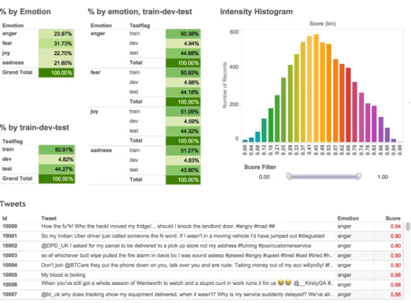
The visualization has three main components: 1. Tables showing the percentage of instances in
each of the emotion partitions (train, dev, test). Hovering over a row shows the corresponding number of instances. Clicking on an emotion filters out data from all other emotions, in all visualization components. Similarly, one can click on just the train, dev, or test partitions to view information just for that data. Clicking again deselects the item.
2. A histogram of emotion intensity scores. A slider that one can use to view only those tweets within a certain score range.
3. The list of tweets, emotion label, and emotion intensity scores.
Notably, the three components are interconnected, such that clicking on an item in one component will filter information in all other components to show only the relevant details. For example, click-ing on ‘joy’ in ‘a’ will cause ‘b’ to show the his-togram for only the joy tweets, and ‘c’ to show only the ‘joy’ tweets. Similarly one can click on the test/dev/train set, a particular band of emotion intensity scores, or a particular tweet. Clicking again deselects the item. One can use filters in combination. For e.g., clicking on fear, test data, and setting the slider for the 0.5 to 1 range, shows information for only those fear–testdata instances with scores ≥ 0.5.
Figure 1: Screenshot of the interactive visualization to explore the Tweet Emotion Intensity Dataset. Available at: http://saifmohammad.com/WebPages/EmotionIntensity-SharedTask.html
8.3 AffectiveTweets Weka Package: Implementation Details
AffectiveTweets includes five filters for convert-ing tweets into feature vectors that can be fed into the large collection of machine learning al-gorithms implemented within Weka. The package is installed using the WekaPackageManager and can be used from the Weka GUI or the command line interface. It uses the TweetNLP library ( Gim-pel et al.,2011) for tokenization and POS tagging. The filters are described as follows.
• TweetToSparseFeatureVector filter: calculates the following sparse features: word n-grams (adding a NEG prefix to words occurring in negated contexts), character n-grams (CN), POS tags, and Brown word clusters.26
• TweetToLexiconFeatureVector filter: calculates features from a fixed list of affective lexicons. 26The scope of negation was determined by a simple
heuristic: from the occurrence of a negator word up until a punctuation mark or end of sentence. We used a list of 28 negator words such as no, not, won’t and never.
• TweetToInputLexiconFeatureVector: calculates features from any lexicon. The input lexicon can have multiple numeric or nominal word– affect associations. This filter allows users to experiment with their own lexicons.
• TweetToSentiStrengthFeatureVector filter: cal-culates positive and negative sentiment intensi-ties for a tweet using the SentiStrength lexicon-based method (Thelwall et al.,2012)
• TweetToEmbeddingsFeatureVectorfilter: calcu-lates a tweet-level feature representation us-ing pre-trained word embeddus-ings supportus-ing the following aggregation schemes: average of word embeddings; addition of word embed-dings; and concatenation of the first k word em-beddings in the tweet. The package also pro-vides Word2Vec’s pre-trained word.27
Once the feature vectors are created, one can use any of the Weka regression or classification algo-rithms. Additional filters are under development.
27
https://code.google.com/archive/p/word2vec/
View publication stats View publication stats