White Rose Research Online URL for this paper:
http://eprints.whiterose.ac.uk/91585/
Version: Accepted Version
Article:
Apablaza, M, Bresson, F and Yalonetzky, G (2016) When more does not necessarily mean
better: Health-related illfare comparisons with non-monotone wellbeing relationships.
Review of Income and Wealth, 62 (S1). S145-S178. ISSN 0034-6586
https://doi.org/10.1111/roiw.12221
© 2015 International Association for Research in Income and Wealth. This is the peer
reviewed version of the following article: Apablaza, M., Bresson, F. and Yalonetzky, G.
(2016), When More Does Not Necessarily Mean Better: Health-Related Illfare
Comparisons with Non-Monotone Well-Being Relationships. Review of Income and
Wealth, 62: S145–S178. doi: 10.1111/roiw.12221, which has been published in final form at
https://doi.org/10.1111/roiw.12221. This article may be used for non-commercial purposes
in accordance with Wiley Terms and Conditions for Self-Archiving.
[email protected] https://eprints.whiterose.ac.uk/ Reuse
Unless indicated otherwise, fulltext items are protected by copyright with all rights reserved. The copyright exception in section 29 of the Copyright, Designs and Patents Act 1988 allows the making of a single copy solely for the purpose of non-commercial research or private study within the limits of fair dealing. The publisher or other rights-holder may allow further reproduction and re-use of this version - refer to the White Rose Research Online record for this item. Where records identify the publisher as the copyright holder, users can verify any specific terms of use on the publisher’s website.
Takedown
If you consider content in White Rose Research Online to be in breach of UK law, please notify us by
Health-related illfare comparisons with
non-monotone wellbeing relationships
Mauricio APABLAZA∗ Florent BRESSON† Gaston YALONETZKY‡September 8, 2015
Abstract
Most welfare studies assume that wellbeing is monotonically related to the variables used for the analysis. While this assumption is reasonable for many dimensions of well-being like income, education, or empowerment, there are some cases where it is defini-tively not relevant, in particular with respect to health. For instance, health status is often proxied using the Body Mass Index (BMI). Low BMI values can capture under-nutrition or the incidence of severe illness, yet a high BMI is neither desirable as it indicates obesity. Usual illfare indices derived from poverty measurement are then not appropriate. This paper proposes illfare indices that are consistent with some situa-tions of non-monotonic wellbeing relasitua-tionships and examines the partial orderings of different distributions derived from various classes of illfare indices. An illustration is provided for child health as proxied by a weight-for-age indicator using DHS data for Bangladesh, Colombia and Egypt during the last few decades.
Keywords: Illfare comparisons, poverty measurement, stochastic dominance,
mono-tonicity, nutrition transition.
JEL Classification: D63, I3.
The authors would like to thank Sabina Alkire, Martine Audibert, Marie-Françoise Renard, Patrick Guillaumont, Suman Seth, participants at the Fifth ECINEQ Meeting, Bari, Italy, July 2013 and the IARIW-IBGE Conference on Income, Wealth and Well-being in Latin America, Rio de Janeiro, Brazil, September, 2013, as well as the two anonymous referees for their helpful comments. The usual disclaimer applies.
∗
OPHI, Oxford; Faculty of Government, Universidad del Desarrollo, Chile; email: [email protected].
† CERDI, École d’Économie, Université d’Auvergne (Clermont-Ferrand 1); email:
1
Introduction
Target 1.C from the Millennium Development Goals states that the proportion of people who suffer from hunger should be halved between 1990 and 2015. Although this objective is unlikely to be met by 2015, the share of undernourished individuals has declined during the period (de Onis et al., 2004, Department of Economic and Social Affairs of the U. N. Secretariat, 2012). For instance, the FAO finds that the share of undernourished people in the developing world fell from about 20% to 15% during the period 1990-2010.1 However, a stylized fact in most developing countries is that progresses concerning undernutrition have often been associated with increase in obesity (Popkin et al., 2012). This so-called nutrition transition raises the issue of a net gain in social welfare with respect to health. Should we consider that the level of welfare in a society has improved if undernutrition has declined but other forms of malnutrition have become more severe? If we want to perform a global assessment of the social progress with respect to nutrition, then we need to render the situations of underweight and overweight individuals socially comparable.
Wellbeing is generally supposed to be monotonically related to the variables used for the analysis in poverty and welfare studies. While this assumption can be deemed rea-sonable for many dimensions of wellbeing like income, education, or empowerment, there are some cases where it is definitively not relevant, in particular regarding health. For instance, health status is often proxied using the Body Mass Index (BMI) in the case of adults,or using weight-for-age or height-for-age in the case of children and adolescents. Low BMI values can capture undernutrition or the incidence of severe illness, yet a high BMI is neither desirable as it indicates obesity. That is why the BMI is usually compared against a left-tail and a right-tail cut-off which work as deprivation lines, e.g. 18.5 kg/m2 and 25 kg/m2, respectively. Estimating aggregate illfare using traditional poverty indices, based on a unique (left-tailed) deprivation line, is therefore not appropriate. Likewise several other health indicators are characterized by the use of two deprivation lines for diagnostic purposes because they relate to situations in which either “having too much” or “too little” is detrimental to health. That is the case of several blood tests, including blood pressure, thyroid function, haemoglobin and total cholesterol.
This paper first proposes illfare indices that are consistent with situations of non-monotonic relationships between wellbeing and its indicators, like the aforementioned examples. These indices are decomposable into two indices that, respectively, measure a concept of “shortfall” illfare and another one of “excess” illfare. While “shortfall” illfare is identical to the traditional understanding of poverty as insufficiency, “excess” illfare refers to wellbeing harmed by suboptimal abundance. The family of indices is described in terms of its fulfillment of desirable axioms, and includes extensions of traditional poverty indices like the Foster-Greer-Thorbecke family, the Clark-Hemming-Ulph family, and the Watts index. For the above purpose we introduce key alterations to the traditional axioms of focus, monotonicity and transfers.
Indices provide precise and useful information as well as a complete ordering of ob-served distributions. However, they are all based on specific underlying welfare functions
1Figures are from the 2012 Millennium Development Goals Report (Department of Economic and Social
(Blackorby and Donaldson, 1980) upon which agreement may not be met. Of course, in the health context, risks of death or severe disease may theoretically be precisely estimated for the different values of the variable under consideration, but it is not so clear how people value such risks in terms of wellbeing. The relationship becomes even more complex once psychological and social aspects of health are taken into account. For these reasons, it is necessary to look for criteria that make it possible to draw robust conclusions about the state of illfare; that is, to obtain results that do not depend on the specific functional forms used to assess illfare. The paper also examines the partial orderings of different distribu-tions, according to sub-families of our class of illfare indices, by deriving the required first and second-order stochastic dominance conditions. We also study the conditions for partial orderings when the experience of one form of illfare (e.g. “shortfall” illfare) is considered to be worse than the other one (e.g. “excess” illfare).
The rest of the paper is organized as follows: The next section introduces the family of non-monotone illfare indices and its associated partial ordering conditions. The third sec-tion proposes stochastic dominance condisec-tions when the two forms of illfare are deemed to have differential effects on wellbeing. Section 4 shows how to compute the standard errors for the family of indices. The fifth section provides an empirical illustration of child health illfare measured by a weight-for-age indicator, and using several Demographic Health Sur-veys (DHS) from Bangladesh, Colombia and Egypt; three large developing countries in South Asia, Latin America and North Africa, respectively. The illustration shows that health-related illfare levels have declined during the periods of analysis for under-5 chil-dren in all countries, but that the overall improvement is partly offset by the increase in obesity. The paper concludes with some final remarks.
2
Non-monotone poverty measurement: The general case
2.1 Two classes of poverty indices with revised versions of the focus,
monotonicity and transfer axioms
Let x describe an individual attribute defined on the domain Ω∶= [ω−, ω+] ⊂ R. Illfare may then be assessed using unidimensional additive poverty indices P(z) that are of the type:
P(z) ∶= ∫ z
ω−π(x,z)dF(x), (1)
where F is the cumulative distribution function (cdf), z ∈ Ω is the poverty line, and the continuous function π∶ Ω × Ω → R+is an individual poverty index such that:
π(x,z)⎧⎪⎪⎪⎨⎪⎪⎪ ⎩
> 0 if x < z,
= 0 otherwise. (2)
Indices of the family (1) satisfy the traditional properties of continuity, anonymity, pop-ulation replication, focus and additive decomposability. Moreover, they also comply with weak monotonicity if ∂π
∂x ⩽ 0. In general the monotonicity axiom enjoys broad consensus and is consistent with poverty assessments based on income.
With indices P(z), illfare is associated with insufficient level of the variable x with regard to a norm corresponding to z. However, the relevant space for conceptualizing wellbeing is rarely the one where attribute x is defined. Indeed, the “failure to achieve certain minimum capabilities” (Sen, 1985) does not systematically mean an insufficient value for x. So, in the space of capabilities, illfare can be defined as a lack of resources but potentially not in the space of x. Considering nutrition, a person is health-deprived if she does not have the ability to get an adequate and balanced diet, regarding her physiological, psychological and social needs. Causes of this inability are diverse, including for instance low income, limited access to diversified sources of nutrients, insufficient information on the importance of a balanced diet, severe diseases or handicaps, and mental disorders. Whatever the precise roots of health-related illfare, we consider them to be the expression of low capabilities.
Here we consider illfare indices that do not exhibit the same behaviour as indices (1) because the underlying relationship between variable x and welfare is not supposed to be monotonic. More specifically, we introduce a set of deprivation lines {zL, zU} ⊂ Ω, with zL< zU, such that:2 π(x;zL, zU) ⎧⎪⎪⎪⎪ ⎪⎪ ⎨⎪⎪⎪ ⎪⎪⎪⎩ > 0 if x < zL, = 0 if x ∈ [zL, zU] > 0 if x > zU , (3)
where π is also a continuous function. Hence here illfare relates to situations in which either “having too much” or “having too little” is detrimental for individual wellbeing. We note at the outset that such non-monotone relationship with respect to health has already been investigated regarding health inequalities (e.g. Dutta, 2007), but, to the best of our knowledge, no tool has yet been proposed for the social assessment of total health illfare.
At the social aggregation level, we consider illfare indices P of the type: P(zL, zU) ∶= ∫ zL ω− π(x;z L, zU)dF(x) + ∫ ω + zU π(x;z L, zU)dF(x). (4) Note, firstly, that the definition of P in equation (1) can be seen as the limiting case zU = ω+ of the definition in equation (4). Secondly, P in equation (4) does not fulfil the traditional definitions of the focus and monotonicity axioms proposed by Sen (1976). A poverty index complies with the focus axiom if the social poverty level does not change when a non-poor person receives more of x. However for any individual with x∈]zL, zU[, there is always an increment κ> 0 such that x + κ ⩾ zU, i.e. the individual falls into illfare. Likewise, the monotonicity axiom usually states that poverty does not increase whenever
2Here we suppose that the same deprivation lines zLand zU can be applied for each individual within
the observed populations, and that they are exogenous with respect to the observed values of x within these populations. The first assumption means that the same thresholds can be applied for each person whatever her sex, age, or any other relevant characteristic. Both for illfare measurement and dominance tests, that assumption can be relaxed, notably by rescaling observed values of x so that all group-specific deprivation lines coincide. The second assumption implies that we are measuring absolute illfare. While this focus is reasonable for physiological dimensions of health, it is admittedly contentious when dealing with psychological and social aspects. For instance, we could posit that obesity becomes a more acute concern when its prevalence is rare than when it is widespread among the population. These considerations are however left aside for future work.
a poor person augments her x. Nevertheless in our setting we posit that increases above the upper deprivation line zU should not decrease illfare. These conflicts are not surprising as the focus and monotonicity axioms are usually defined for indices in the shape of equa-tion (1). Since the focus and monotonicity axioms express simple and desirable properties, it is worth proposing new definitions for these axioms befitting our specific framework. Formally:
Axiom(FOC). PA(zL, zU) = PB(zL, zU) if distribution B is obtained from distribution A by adding κ∈ R to any observed value x ∈]zL, zU[ such that x + κ ∈]zL, zU[.
Axiom (MON). PA(zL, zU) ⩽ PB(zL, zU) if distribution B is obtained from distribution A i) by subtracting κ> 0 to any observed value x ∈ [ω−, zL] such that x − κ ∈ Ω, or ii) by adding κ> 0 to any observed value x ∈ [zU, ω+] such that x + κ ∈ Ω.
Axioms FOC and MON are thus defined in order to preserve the spirit underlying their usual definitions. FOC assumes that a change in x for a non-deprived person does not change illfare as long as the person remains outside the illfare domain. The monotonic-ity axiom is usually defined to state that movements towards the poverty line for a poor person do not increase poverty. That is exactly what axiom MON states for illfare. To elu-cidate that point, let us introduce the concepts of “shortfall" illfare and “excess" illfare. The former refers to an insufficient amount of a wellbeing attribute x, usually judged by com-paring against the left-tail deprivation line zL. By contrast, “excess" illfare is the situation of an excessive, and detrimental, amount of a wellbeing attribute, or indicator, e.g. the BMI; which is determined by comparing x against the right-tail deprivation line zU. Then our monotonicity axiom states that both a decrease in x for a “shortfall" illfare person, and an increase in x for an “excess" illfare person do not decrease overall illfare.
We can now define the following class of non-monotone illfare indices:
Π1(zL+, zU−) ∶=⎧⎪⎪⎪⎪⎪⎨ ⎪⎪⎪⎪⎪ ⎩ PRRRRRRRRRR RRRRR RR zL∈ [ω−, zL+], zU ∈ [zU−, ω+], zL+⩽ zU− π(x;zL, zU) ∈ ˆC1 π(1)(x;zL, zU) ⩽ 0, ∀x < zL, and π(1)(x;zL, zU) ⩾ 0, ∀x > zU ⎫⎪⎪⎪⎪ ⎪⎬ ⎪⎪⎪⎪⎪ ⎭ , (5) where π(1)(x;zL, zU) ∶= ∂π ∂x and ˆC
s is the set of functions that are s times piecewise dif-ferentiable on Ω. Members of Π1(zL+, zU−) fulfil FOC and MON as defined above. They also comply with the traditional anonymity, additive decomposability, continuity and pop-ulation replication invariance axioms. Anonymity states that x is the sole characteristic explaining why two individuals could exhibit differing values of π. Thus, other characteris-tics like age, household size, ethno-linguistic features, or gender, should not be considered when assessing illfare. Additive decomposability means that overall social illfare is the sum of individual illfare measures, a property that is desirable within our framework in order to assess the relative contribution of “shortfall” and “excess” illfare to overall illfare. Continuity at the deprivation line is the result of the second condition in (5), and is neces-sary to prevent small measurement errors from producing non-marginal variations in the estimated illfare level.3 Finally, the population invariance principle states that replicat-ing each member of the population the same number of times does not change the level
condi-of illfare, so that population condi-of different size can be compared in terms condi-of illfare. Fulfil-ment of this property requires the social illfare function to be an arithmetic average of the individual measures.
Interesting examples of P ∈ Π1(zL+, zU−) are the following extensions of the traditional Foster et al.’s (1984) poverty indices:
F GTβ,αL,αU(z L, zU) ∶= ∫ z L ω− ( zL− x zL− ω−) αL dF(x) + β ∫ ω + zU ( x− zU ω+− zU) αU dF(x), (6) with β> 0, αL⩾ 1, and αU ⩾ 1. The family FGTβ,αL,αU also includes the headcount index for
αL= αU = 0. The headcount index is not a member of Π1(zL+, zU−), as it is not continuous within the illfare domain; but provides useful information regarding the prevalence of illfare within the population. β is a weighing parameter that gives more emphasis on “shortfall” illfare for β ∈ (0,1) and on “excess” illfare for β > 1. The parameters αLand αU regulate the index’s sensitivity to extreme forms of deprivation. Likewise, we can easily propose extensions to other traditional poverty indices, e.g. the Watts, or those from the Clark-Hemming-Ulph family.
These indices are relative indices as the size of individual shortfalls or excesses is normalized by the corresponding value for the maximum shortfall or excess, respectively. Alternatively, one may use, for instance, the following absolute version of the F GTβ,αL,αU:
F GTβ,αA L,αU(z L, zU) ∶= ∫ z L ω− (z L− x)αL dF(x) + β ∫ ω+ zU (x − z U)αU dF(x), (7) with αL⩾ 0 and αU ⩾ 0.
Here we note that Jolliffe (2004) proposed a measure of the social burden of overweight related to the Foster et al.’s (1984) family of poverty indices. More specifically, using our own notations, the proposed measure was:
OWαU(z U) ∶= ∫ ω + zU ( x− zU zU ) αU dF(x). (8)
Of course, indices OWαU differs from F GTβ,αL,αU as the former only considers
over-weight. But also the normalization of “excesses” is also performed differently between the two families: While “excesses” are normalized by the threshold zU in OW
αU, F GTβ,αL,αU
uses the maximum “excess” ω+− zU. Therefore the two families may not provide the same ordering of “excess” illfare for αU ⩾ 2. Moreover, our normalization approach is more appro-priate for comparability purposes between “loss” and “excess” illfare, since normalization by the reference thresholds would result in relatively lower relative gaps in the “excess” do-main as they would be associated with a larger threshold. Finally, indices from F GTβ,αL,αU
fulfil an additional property of translation invariance, whereby the illfare level is left un-changed after incrementing each value x, the bounds ω− and ω+, and the thresholds zL and zU by the same amount.
tions. Consequently, the conditions expressed below in Proposition 1 could also be applied to a broader class of illfare indices that may not respect continuity at the deprivation line. On the other hand, continuity is desirable for second order dominance conditions. On this specific point for poverty analysis, see for instance Zheng (1999) and Araar and Duclos (2006).
The index OWαU(z
U) was also proposed as a measure of richness by Peichl et al. (2010). The authors also introduced concave indices (with αU ∈]0;1[) that do not fit our framework regarding the effects of progressive transfers (see below).
Following Sen (1976) we may prefer illfare indices to be sensitive to inequalities be-tween those individuals experiencing illfare situations. Such distribution-sensitive indices usually comply with a transfer axiom stating that progressive transfers between two in-dividuals in illfare should decrease, or at least not increase, the illfare level.4 However, it is worth noting that, contrary to indices of the type (1), Pigou-Dalton transfers within our framework have to be considered over a non-convex set since the illfare domain is defined by the union of non-contiguous intervals. Consequently, we may consider three cases: i) when both people are experiencing “shortfall” illfare; ii) when both are in “excess” illfare; and iii) when the two persons belong to these different groups. The first two cases can be handled just like rank-preserving progressive transfers in the traditional poverty literature (i.e. based on (1)). In the third case, a transfer from the “excess” illfare person to the “shortfall” illfare person means wellbeing improvements for both people, therefore it can be addressed using MON. Hence the apparent inability of our transfer axiom to deal with transfers between any pair of individuals in illfare situations is not a a matter of concern, since our illfare indices comply with MON.
The transfer axiom can thus be presented in the following manner:
Axiom(TRA). PA(zL, zU) ⩾ PB(zL, zU) if distribution B is obtained from distribution A by transferring κ> 0 from individual i to individual j such that {xi, xj} ⊂ [ω−, zL] or {xi, xj} ⊂ [zU, ω+], and ∣x
i− xj∣ ⩾ ∣(xi− κ) − (xj+ κ)∣.5
Note that members from the class F GTβ,αL,αU(z
L, zU) respect this transfer axiom only for αL⩾ 1 and αU ⩾ 1.
If we want illfare not to increase in the aftermath of Pigou-Dalton transfers, then we can consider the following class of indices satisfying TRA:
Π2(zL+, zU−) ∶=⎧⎪⎪⎨⎪⎪ ⎩P ∈ Π 1(zL+, zU−)RRRRR RRRRR R π(x;zL, zU) ∈ ˆC2 π(2)(x;zL, zU) ⩾ 0, ∀x ∈ Ω ⎫⎪⎪ ⎬⎪⎪ ⎭, (9) where π(2)(x;zL, zU) ∶= ∂2π
(∂x)2. The first condition is a technical requirement for the
deriva-tion of dominance condideriva-tions since it ensures second-order derivatives of π exists for most value of x∈ Ω. The second condition in (9) captures the requirement regarding the sensitiv-ity of the social poverty function to progressive transfers. In formal terms, the additivsensitiv-ity of P associated with the second condition in (9) means that members from Π2(zL+, zU−) are S-convex in “shortfall” illfare values of x and also S-convex in “excess” illfare values of x. Both conditions mean finally that the marginal gain in the improvement of the situation of a person in illfare decreases and tends to zero as she moves closer to her deprivation
4Admittedly, some wellbeing outcomes, e.g. those pertaining to health, are not easily transferrable in the
way income is. So the concept of "transfers" is used only figuratively in these cases of illfare, as it is still useful to assess sensitivity to inequality between individuals experiencing illfare situations. We thank an anonymous referee for highlighting this point.
5TRA could alternatively be introduced in a strong sense, in which case we would state that: P
A(zL, zU) >
PB(zL, zU) if distribution B is obtained from distribution A by transferring κ > 0 from individual i to
individ-ual j such that {x, x} ⊂ [ω−
, zL] or {x, x } ⊂ [zU
, ω+
line. It can be regarded as a desirable property as it rewards policy efforts focused on individuals experiencing severe “shortfalls” or “excesses.”
2.2 Partial orderings
The limited set of conditions expressed for the definition of the classes Π1(zL+, zU−) and Π2(zL+, zU−) leaves the door open for a wide variety of illfare indices; modified FGT indices are only suggestions of appropriate indices within our non-monotone framework. In the following paragraphs, we derive full robustness conditions for ordinal illfare comparisons based on stochastic dominance conditions; that is, results that do not hinge on specific indices or deprivation lines choices. We first propose a set of criteria for the class of illfare measures Π1.
Proposition 1.
PA(zL, zU) ⩽ PB(zL, zU)∀P ∈ Π1(zL+, zU−) (10)
iff FA(x) ⩽ FB(x) ∀x ∈ [ω−, zL+[ (11) and FA(x) ⩽ FB(x) ∀x ∈]zU−, ω+], (12) where F(z) ≡ Pr[x ⩾ z] = 1 − F(z) is the survival function.
Proof. See appendix A.1 ∎
The first-order dominance relationship presented in Proposition 1 states that illfare in distribution A is not higher than in distribution B if the value of the “shortfall” illfare headcount index is never larger for distribution A for each value of the deprivation line within the largest admissible “shortfall” illfare domain[ω−, zL+], and if the “excess” illfare headcount is never higher in A for each deprivation line within the largest admissible “excess” illfare domain[zU−, ω+]. To illustrate numerically the conditions in Proposition 1, let us consider distributions A ∶= (1,4,6,9,12, 14) and B ∶= (1,4,7,8,13, 14), and assume zL+= 5 and zU− = 10. Using Proposition 1, it can easily be seen that distribution A never shows more illfare than distribution B for all indices in Π1and all pairs of deprivation lines {zL, zU} /⊂ (zL+, zU−) since FA(x) = FB(x) ∀x ∈ [ω−, 5] ∪ [10,12[∪[13,ω+] but FA(x) > FB(x) ∀x ∈ [12,13[.
Strictly speaking, conditions (11) and (12) could be checked over their whole poverty subdomains, i.e. [ω−, zL+] and [zU−, ω+], respectively, only if the cumulative and survival functions are deemed continuous. This is the standard practice in several seminal pa-pers in the poverty dominance literature including Atkinson (1987, 1992), and Duclos and Makdissi (2004). However, in situations like our numerical example we have cumulative and survival functions which are, in fact, discontinuous, step functions. Therefore, in these cases, it is easy to show that condition (11) should hold for all x∈ [ω−, zL+[, while condition (12) should hold for all x ∈]zU−, ω+]. Note that a similar remark, pertaining to whether and when the conditions may be checked in the deprivation lines, also applies to the con-ditions in propositions (3), (5), and (7) below. Considering restricted continuity instead of continuity, that is leaving the door open for the use of indices that are likely to show
discontinuities at thresholds zLor zU, would also make it necessary to check inequalities (11) and (12) at zL+and zU−, respectively.
It is worth noting that corollary results ensue directly from Proposition 1. Let x be a vector of values for the variable x and #(x) be the number of elements of x. Then, it can easily be checked that there is a first-order dominance relationship between A and B ∀P ∈ Π1(zL+, zU−) if ∃ˆx ∈]zL+, zU−[#(ˆx)such that FAand FBcross only at the sole values in ˆ
xand #(ˆx) is an odd number. Considering our framework, dominance relationships can be observed with any odd number of crossings as long as they happen outside the illfare domain. In the same spirit, if zL+ = zU− = ˜z, distribution A dominates distribution B at the first order ∀P ∈ Π1(zL+, zU−) if and only if FA and FB cross only once and at ˜z. In the case of a single crossing, this second corollary result states that the crossing value is not necessarily the average value of x but can be any other value that is consistent with admissible definitions of the maximum illfare domain.
Proposition 1 is reminiscent of famous results from the literature on risk (Rothschild and Stiglitz, 1970) and inequality (Atkinson, 1970) measurement as the distribution that shows more illfare also exhibits more weight at the tails of its distribution. However, corollary results show that our dominance conditions are less restrictive since risk and inequality dominance conditions are defined for the distributions of the variable x after normalization with respect to the mean, or for distributions with the same mean. On the other hand, risk and inequality usual dominance conditions allow for crossings within the illfare domain. The linkages with second-order dominance tests will be investigated in the next paragraphs.
The familiarized reader will note that condition (12) is related to the first-degree afflu-ence ordering of Michelangeli et al. (2011). These authors also proposed a second degree affluence ordering corresponding to condition (15) in Proposition 2. Nevertheless our paper differs from Michelangeli et al. (2011) since the authors do not consider the joint burden of having individuals that have too little and individuals that have too much as they focus on affluence. Moreover, in our framework “excess” is regarded as a social bad while it seems that affluence is regarded as a social good by Michelangeli et al. (2011).
Proposition 1 only provides a partial ordering for any pair of distributions defined on the domain Ω. In other words, the results with empirical implementations of the test are likely to be non-conclusive for a significant portion of the performed comparisons as it is possible to observe crossings of the cumulative distribution functions within the illfare domain. Hence it can be useful to add restrictions regarding the behaviour of illfare indices in terms of their sensitivity to progressive transfers, and then focus on members of the subclass Π2.
The conditions for subclass Π2 entail manipulating two different functions that ac-cumulate gaps from the boundaries of the domain of x, yielding integrals of cumulative distribution and survival functions respectively. Let G(z) ∶= ∫z
ω−F(x)dx = ∫ z ω−(z − x)dF(x) and G(z) ∶= ∫ω+ z F(x)dx = ∫ ω+
z (x−z)dF (x). The function G(z) is known in the literature on poverty and wellbeing dominance as the absolute poverty gap index, and gives the mean value of the censored gaps max{0,z−x} observed in the population. The function G(z) does not average shortfalls but excesses with respect to the value z, that is max{0,x − z}. Then
we show:
Proposition 2.
PA(zL, zU) ⩽ PB(zL, zU)∀P ∈ Π2(zL+, zU−) (13)
iff GA(x) ⩽ GB(x) ∀x ∈ [ω−, zL+] (14) and GA(x) ⩽ GB(x) ∀x ∈ [zU−, ω+]. (15)
Proof. See appendix A.2 ∎
The first part of the conditions presented in Proposition 2 is identical to the one sug-gested in Atkinson (1987) and Foster and Shorrocks (1988): for each value of x below zL+ the value of the absolute poverty gap index should never be larger for population A than for population B. The second part considers the cumulative “excesses” and states that for illfare not to be higher in population A, the value of the average excesses should be lower for population A than for population B, for every value of x above the upper deprivation line zU−.
Finally, since we are dealing with additively decomposable illfare indices, we may dis-tinguish two parts in the overall illfare level, that is the one corresponding to the presence of individuals within the bottom part of the illfare domain[ω−, zL] and the one correspond-ing to those people whose value of x is above the upper deprivation line zU. Overall illfare is consequently the sum of “shortfall” and “excess” illfare. Therefore we can focus on each group separately and then use only the corresponding condition in Propositions 1 and 2 to check whether a robust ordering can be obtained for the sole “shortfall” (“excess”) illfare component when comparing two distributions. Using the example of distributions A and B in page 8, we can see that both populations show the same level of “shortfall” illfare but that “excess” illfare is robustly larger in population B.
3
The case of comparable deprivations
“Shortfall” and “excess” illfare may be due to different causes, and result in contrasted forms of wellbeing shortfalls. Yet we might feel sometimes that both types do not deserve the same attention when estimating overall illfare. However, no a priori ordering of the situation of a “shortfall” illfare person and an “excess” illfare person can be performed directly as both people exhibit different values for the attribute x. In order to enhance the comparability of the two illfare situations, it is thus useful to move from variable x to a common space. Let assume that there is a strictly decreasing and continuous function g∶ [zU, a] → [ω−, zL] that makes values in the “excess” domain below a directly comparable with values in the “loss” domain. Then the ordering power of the previous stochastic dominance tests can be enhanced by assuming that the sign of π(g(x);zL, zU)−π(x;zL, zU) does not change ∀x ∈ [zU, a]. Of course, many rival functional forms can be proposed for g and the appropriate form is very likely to rely on the chosen wellbeing attribute. In the present paper we will consider two intuitive functional forms but it is worth noting that the next propositions can easily be adapted for the use of different functional forms for g.
As in Fisher and Spencer (1992) and Lambert and Zoli (2012), it may first be worth considering indices defined with respect to distances (gaps) from the closest reference line for each individual, and then bring in additional assumptions regarding the relative size of well-being losses for individuals with different characteristics albeit showing the same gap. Let the absolute gap δ∈ R+be defined as:
δ∶= ⎧⎪⎪⎪⎪ ⎪⎪ ⎨⎪⎪⎪ ⎪⎪⎪⎩ zL− x if x < zL 0 if x∈ [zL, zU] x− zU if x> zU . (16)
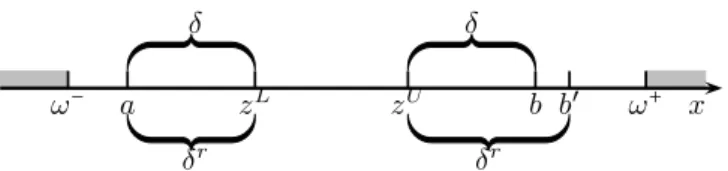
[Insert Figure 1 here.]
Figure 1 shows the situation of two individuals, one is a “shortfall” illfare person with x= a and the other one is an “excess” illfare person with x = b. As the figure shows, both individuals exhibit the same absolute gap δ. That is why: b= zL+ zU− a. However, if we assume that the situation of the “excess” illfare person cannot be regarded as severe as the situation of the “shortfall” illfare person, then we should obtain π(a;zL, zU) ⩾ π (b;zL, zU). If this behaviour is deemed reasonable for every potential value of δ, that is, given x⩽ zL for all{x,zL+ zU− x} ⊂ Ω, we can then consider the following subclass of illfare indices:
˜ Π1(zL+, zU−) ∶=⎧⎪⎪⎨⎪⎪ ⎩P RRRRR RRRRR R P ∈ Π1(zL+, zU−) ∣π(1)(x,zL, zU)∣ ⩾ π(1)(zL+ zU− x,zL, zU) ∀x ⩽ zLs.t.{x,zL+ zU− x} ⊂ Ω ⎫⎪⎪ ⎬⎪⎪ ⎭. (17) The first condition in (17) states that members from ˜Π1(zL+, zU−) comply with the prop-erties of indices from Π1(zL+, zU−). The second condition defines the specificity of these indices, stating that the marginal gain from improving the situation of an “excess” illfare person is never greater than the marginal gain for a “shortfall” illfare person with the same gap. It can easily be noted that, in conjunction with positing a zero poverty level at the deprivation lines, our additional assumption on the first-order derivatives of π im-plies π(x;zL, zU) ⩾ π (zL+ zU− x;zL, zU).Members of ˜Π1(zL+, zU−) include, for instance, the indices F GTA
β,αL,αU(z
L, zU) for which β ∈ (0,1) and α
L= αU.
Considering different groups of individuals in a way that yields different individual ill-fare assessments for a given gap is not a new idea. Indeed, our framework is reminiscent of the literature on monetary poverty comparisons with differences in needs associated with particular attributes of individuals, e.g. their household sizes (Bourguignon, 1989, Atkin-son, 1992, Jenkins and Lambert, 1993, Chambaz and Maurin, 1998, Duclos and Makdissi, 2005, Lambert and Zoli, 2012). These studies show that the ordering power of stochas-tic dominance procedures can be increased when simple assumptions are made about the difference between the individual poverty indices corresponding to two different groups. Here, we suggest that, in many cases, a similar assumption can be made regarding the situation of the “shortfall” and the “excess” illfare persons.
Up to now, we have considered social illfare indices whose individual indices are based on absolute deviations from the deprivation lines. However, a usual practice is to quantify deprivations with relative gaps, e.g. as in the family of measures proposed in equation (6).
That is, we can use δrsuch that: δr∶= ⎧⎪⎪⎪⎪ ⎪⎪ ⎨⎪⎪⎪ ⎪⎪⎪⎩ zL−x zL−ω− if x< z L 0 if x∈ [zL, zU] x−zU ω+−zU if x> z U . (18)
If comparability of the two forms of illfare is based on relative gaps, then we must consider the following subclass of illfare indices:
˜ Π1r(zL+, zU−) ∶=⎧⎪⎪⎨⎪⎪ ⎩P RRRRR RRRRR RR P ∈ Π1(zL+, zU−) ∣π(1)(x,zL, zU)∣ ⩾ π(1)(zU+ zL−x zL−ω−(ω +− zU),zL, zU) ∀x ⩽ zL ⎫⎪⎪ ⎬⎪⎪ ⎭. (19) In principle, when zL− ω−= ω+− zU, illfare comparisons are not affected by a change from absolute gaps to relative gaps. However, in other cases like the one in Figure 1, such a change affects illfare orderings when additional assumptions are made regarding the relative contribution of “shortfall” and “excess” illfare to overall illfare. Using relative gaps δr, instead of absolute gaps δ, when performing the first-order and second-order dominance checks described in Proposition 1 and 2, does not change the results. Yet different results may ensue for the propositions introduced in the next pages since relative gaps do not correspond to the same values of absolute gaps when zL−ω−≠ ω+−zU. Moreover, dominance results with relative gaps are likely to be contingent upon the choices for the values of ω− and/or ω+.
3.1 Linked deprivation lines
It is worth stressing that, for a “shortfall” value a and an “excess” value b to be directly com-parable, both should show the same distance δ or δrfrom their respective deprivation line. This point is important because stochastic dominance is often performed in order to check the robustness of comparisons to changes in deprivation lines. However, when consider-ing gap dominance relationships, each couple(zL, zU) defines all the pairwise comparable values a and b within the “shortfall” and “excess” illfare domains. For instance, increasing zLby κ (κ∈ R+with κ< zU− zL) while leaving zU unchanged implies that the absolute gap δ= x2− zU does not make x2directly comparable with x1but with x1+ κ. Consequently, re-sults obtained when comparing distributions A and B with the vector of deprivation lines (zL, zU) may not hold when using the vector (zL+ κ,zU) as the latter refers to different sets of pairwise comparable values of the wellbeing attribute.
On the other hand, if zL is increased by a given quantity κ and zU decreased by the same amount (with, of course, 2κ< zU− zL), the value of the gap for a and b would raise by the same amount. Therefore the resulting absolute gap δ+ κ would still be associated with the same values of x, thereby leaving the correspondences between the “shortfall” illfare and “excess” illfare domains unchanged. With the assumption that a “shortfall” never yields less illfare than the corresponding “excess” given δ, one can consider the fulfilment of the following conditions in order to ensure ethically robust orderings for any members
of the class ˜Π1of illfare indices:6
Proposition 3.
a) PA(zL, zU) ⩽ P
B(zL, zU) ∀P ∈ ˜Π1(zL+, zU−), zL+−zL= zU−zU−= κ, and κ ∈ [0,min{zL+− ω−, ω+− zU−}[
iff FA(x) ⩽ FB(x) ∀x ∈ [ω−, zL+[ (20)
and FA(x) + FA(zL++ zU−− x) ⩽ FB(x) + FB(zL++ zU−− x) ∀x ∈]zU−, ω+]. (21) b) PA(zL, zU) ⩽ PB(zL, zU) ∀P ∈ ˜Π1r(zL+, zU−), z L+−zL zL+−ω− = zU−zU − ω+ −zU − = κ ∈ [0,1[ iff FA(x) ⩽ FB(x) ∀x ∈ [ω−, zL+[ (22) and FA(x) + FA(zL+− x− z U− ω+− zU−(z L− ω−)) ⩽ FB (x) + FB(zL+− x− zU− ω+− zU−(z L− ω−)) ∀x ∈]zU−, ω+]. (23)
Proof. See appendix B.1. ∎
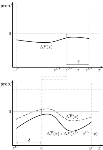
[Insert Figure 2 here.]
Proposition 3 is a sequential dominance criterion in the spirit of those proposed in the aforementioned studies (in particular, the part on absolute gaps bears resemblance to proposition 1(i) of Lambert and Zoli (2012)). First, condition (20) is the same as in Proposition 1 and states that the share of the population that experiences “shortfall” ill-fare, i.e. the neediest group, should be lower in population A than in B at each value of x⩽ zL+, for illfare to be lower in the former population. The second condition does not make any difference between “shortfall” and “excess” gaps since both are brought together for a comparison of the cdf of gaps for each possible value of δ or δr within the illfare domain (expressed in terms of gaps). Figure 2 illustrates these conditions when comparability is assumed using absolute gaps. An interesting feature of the subclasses ˜Π1 and ˜Π1r is that a relatively worsening outlook regarding “excess” illfare can be compensated by relatively positive trends regarding the “shortfall” illfare people.
Let us illustrate that point with another example. Consider now distributions A ∶= (1,4,8,8,12) and B ∶= (1,2,7,7,11), still with zL+ = 5 and zU− = 10. It can easily be seen that Proposition 1 does not hold since A exhibits less “shortfall” illfare than B but more “excess” illfare. However, if we suppose that a given absolute gap δ yields more intense forms of illfare in the “shortfall” domain than in the “excess” domain, the two distributions can be ordered. Condition (20) is satisfied for each observed gap in the “shortfall” illfare domain. For the second condition, disregarding the nature of the gaps, we respectively obtain the following vectors of gaps(0,0,1,2,4) and (0,0,1,3,4) and it can then be seen that FA(x)+FA(5+10−x) = FB(x)+FB(5+10−x) ∀x ∈ [10,12]∪]13,ω+], but FA(x)+FA(5+10−x) < FB(x) + FB(5 + 10 − x) ∀x ∈]12,13], so that condition (21) is also respected and we can
6A similar assumption is made in Lambert and Zoli (2012) for income poverty comparisons with
group-specific poverty lines. As the authors consider gap-dominance relationships, they investigate the case of shifting all group-specific poverty lines up by the same amount.
conclude that A exhibits less illfare than B. It is also important to stress that the ordering is left intact if the lower and upper deprivation lines are respectively decreased and raised by the same amount. For instance, if zL= zL+−1 and zU = zU−+1, we obtain the two vectors of gaps(0,0,0,1,3) and (0,0,0,2,3) and it can be seen that A still shows less illfare than distribution B whatever the precise functional form of P within ˜Π1(zL+, zU−).
It is worth noting that the sequential dominance conditions expressed in Proposition 3 differ from those proposed in the sequential dominance literature (a notable exception is Bourguignon, 1989) as the illfare domain for the neediest group is not necessarily larger than the one for the less needy group. Indeed, if zL+−ω−⩽ ω+−zU−, the size of the absolute gaps can be larger within the “excess” illfare domain than within the “shortfall” illfare domain, so that for values of x∈]zL++ zU−− ω−, ω+] it is not possible for “shortfall” illfare situations to compensate for “excess” illfare situations in condition (21).
As with the class of illfare indices Π1, we can also assume that indices from Π2 are more averse to inequality at the bottom of the distribution than at its upper tail. We then consider the classes ˜Π2and ˜Π2rsuch that:
˜ Π2(zL+, zU−) ∶=⎧⎪⎪⎨⎪⎪ ⎩P RRRRR RRRRR R P ∈ ˜Π1(zL+, zU−) ∩ Π2(zL+, zU−) π(2)(x,zL, zU) ⩾ π(2)(zL+ zU− x,zL, zU) ∀x ⩽ zLs.t.{x,zL+ zU− x} ⊂ Ω ⎫⎪⎪ ⎬⎪⎪ ⎭, (24) ˜ Π2r(zL+, zU−) ∶=⎧⎪⎪⎨⎪⎪ ⎩ P RRRRRRRRRR RR P ∈ ˜Π1r(zL+, zU−) ∩ Π2(zL+, zU−) π(2)(x,zL, zU) ⩾ π(2)(zU+zzLL−ω−x−(ω +− zU),zL, zU,) ∀x ⩽ zL ⎫⎪⎪ ⎬⎪⎪ ⎭ . (25)
The first condition in (24) (in (25)) states that members from ˜Π2(zL+, zU−) (˜Π2r(zL+, zU−)) form a common subclass of both ˜Π1(zL+, zU−) (˜Π1r(zL+, zU−)) and Π2(zL+, zU−). The second line in (24) and (25) states that the marginal gains from improving the situation of a “shortfall” illfare person decrease more rapidly than for the “excess” illfare people. The corresponding dominance criteria for the two classes of illfare indices are:
Proposition 4.
a) PA(zL, zU) ⩽ P
B(zL, zU) ∀P ∈ ˜Π2(zL+, zU−), zL+− zL = zU − zU− = κ, and κ ∈ [0,min{zL+− ω−, ω+− zU−}[
iff GA(x) ⩽ GB(x) ∀x ∈ [ω−, zL+] (26)
and GA(x) + GA(zL++ zU−− x) ⩽ GB(x) + GB(zL++ zU−− x) ∀x ∈ [zU−, ω+]. (27) b) PA(zL, zU) ⩽ PB(zL, zU) ∀P ∈ ˜Π2r(zL+, zU−), z L+−zL zL+−ω− = zU−zU − ω+ −zU − = κ ∈ [0,1[ iff GA(x) ⩽ GB(x) ∀x ∈ [ω−, zL+] (28) and GA(x) + GA(zL+− x− z U− ω+− zU−(z L− ω−)) ⩽ GB (x) + GB(zL+− x− zU− ω+− zU−(z L− ω−)) ∀x ∈ [zU−, ω+]. (29)
Proof. See appendix B.2. ∎
proposi-tion 1(ii) in Lambert and Zoli (2012).
3.2 Independent deprivation lines
While Propositions 3 and 4 allow for a large set of choices for the deprivation lines(zL, zU), we may feel that the conditions linking zL and zU, given zL+ and zU−, are too restrictive, since they do not make it possible to choose freely the vector of deprivation lines within some set[zL−, zL+]×[zU−, zU+] of admissible pairs of deprivation lines. If one desires to get such flexibility, it is then necessary to consider the following propositions:
Proposition 5.
a) PA(zL, zU) ⩽ PB(zL, zU) ∀P ∈ ˜Π1(zL+, zU−), zL∈ [zL−, zL+], and zU ∈ [zU−, zU+] iff FA(x) ⩽ FB(x) ∀x ∈ [ω−, zL+[ (30) and FA(x) + FA(zL+ zU− x) ⩽ FB(x) + FB(zL+ zU− x) (31)
∀x ∈]zU, ω+], zL∈ [zL−, zL+], and zU ∈ [zU−, zU+]. b) PA(zL, zU) ⩽ P
B(zL, zU) ∀P ∈ ˜Π1r(zL+, zU−), zL∈ [zL−, zL+], and zU∈ [zU−, zU+]
iff FA(x) ⩽ FB(x) ∀x ∈ [ω−, zL+[ (32) and FA(x) + FA(zL− x− z U ω+− zU(z L− ω−)) ⩽ FB(x) + FB(zL− x− zU ω+− zU(z L− ω−)) (33) ∀x ∈]zU, ω+], zL∈ [zL−, zL+], and zU ∈ [zU−, zU+]. Proposition 6.
a) PA(zL, zU) ⩽ PB(zL, zU) ∀P ∈ ˜Π2(zL+, zU−), zL∈ [zL−, zL+], and zU ∈ [zU−, zU+] iff GA(x) ⩽ GB(x) ∀x ∈ [ω−, zL+] (34) and GA(x) + GA(zL+ zU− x) ⩽ GB(x) + GB(zL+ zU− x) (35)
∀x ∈ [zU, ω+], zL∈ [zL−, zL+], and zU ∈ [zU−, zU+].
b) PA(zL, zU) ⩽ PB(zL, zU) ∀P ∈ ˜Π2r(zL+, zU−), zL∈ [zL−, zL+], and zU∈ [zU−, zU+]
iff GA(x) ⩽ GB(x) ∀x ∈ [ω−, zL+] (36) and GA(x) + GA(zL− x− z U ω+− zU(z L− ω−)) ⩽ GB(x) + GB(zL− x− zU ω+− zU(z L− ω−)) (37) ∀x ∈ [zU, ω+], zL∈ [zL−, zL+], and zU ∈ [zU−, zU+].
Proof. See appendices B.1 and B.2. ∎
While these latter Propositions provide more robust conditions than those given by Propositions 3 and 4, it is easy to realize that they are computationally intensive. From a practical point of view, note that, since Propositions 5 and 6 are generalizations of Propo-sitions 3 and 4, respectively, the conditions in the former will never be met if those in the
latter are not fulfilled. Hence checking first the easily implementable conditions (20) and (21), is advisable.
It is worth stressing that Propositions 5 and 6 are generalizations of Propositions 3 and 4 only in very specific cases (for instance it is required zL−= ω−and zU+= ω+), because the corresponding sets of poverty lines are generally not nested. However, we argue that Propositions 5 and 6 are “more robust” from an ethical point of view because they are more flexible regarding the choice of the poverty lines.
For absolute gaps, Lambert and Zoli (2005) have also derived similar conditions in which group-specific poverty lines vary independently in non-overlapping ranges, but in the different conceptual framework of monotonic poverty and several groups with different needs.
That said, conditions (31) and (35) can also be expressed in a different manner that renders their implementation more manageable, in the spirit of Bourguignon (1989). Let ϕ1(x) be the maximum value of the difference FA(y) − FB(y) for a given value of x ∈ [zU−, ω+] where y denotes the value of the wellbeing attribute that exhibits the same abso-lute gap within the “shortfall” illfare domain as x does within the “excess” illfare domain, that is:
ϕ1(x) = max y∈Λ(x)F
A(y) − FB(y), (38)
where Λ(x) = [ max{ω−, zL−+ zU−− x},zL+− max{0,x − zU+}] is the part of the “loss” domain where the counterpart of the “excess” value x is likely to be found given the chosen bounds for the two deprivation lines (a detailed explanation of the derivation of Λ(x) can be found in Appendix B.3.1). In the same spirit, we define ϕ2(x) as:
ϕ2(x) = max y∈Λ(x)∫ y ω−F A(t) − FB(t)dt. (39) Finally, let ϕr
k(x), k = 1,2, be the counterpart of ϕk(x) with relative gaps. The sole difference with respect to the expressions given in equations (38) and (39) is that Λ(x) is replaced by Λr(x) = [zL−+ zU −−x ω+ −zU −(zL−− ω−),zL++ min {0, zU +−x ω+ −zU +(zL+− ω−)}] (a detailed
explanation of the derivation of Λr(x) can be found in Appendix B.3.2). Propositions 5 and 6 can then be alternatively expressed as:
Proposition 7.
a) PA(zL, zU) ⩽ PB(zL, zU) ∀P ∈ ˜Π1(zL+, zU−), zL∈ [zL−, zL+], and zU ∈ [zU−, zU+]
iff FA(x) ⩽ FB(x) ∀x ∈ [ω−, zL+[ (40) and FA(x) − FB(x) + ϕ1(x) ⩽ 0 ∀x ∈]zU−, ω+]. (41) b) PA(zL, zU) ⩽ PB(zL, zU) ∀P ∈ ˜Π1r(zL+, zU−), zL∈ [zL−, zL+], and zU ∈ [zU−, zU+]
iff FA(x) ⩽ FB(x) ∀x ∈ [ω−, zL+[ (42) and FA(x) − FB(x) + ϕr1(x) ⩽ 0 ∀x ∈]zU−, ω+]. (43)
a) PA(zL, zU) ⩽ PB(zL, zU) ∀P ∈ ˜Π2(zL+, zU−), zL∈ [zL−, zL+], and zU ∈ [zU−, zU+]
iff GA(x) ⩽ GB(x) ∀x ∈ [ω−, zL+] (44) and GA(x) − GB(x) + ϕ2(x) ⩽ 0 ∀x ∈ [zU−, ω+]. (45) b) PA(zL, zU) ⩽ PB(zL, zU) ∀P ∈ ˜Π2r(zL+, zU−), zL∈ [zL−, zL+], and zU ∈ [zU−, zU+]
iff GA(x) ⩽ GB(x) ∀x ∈ [ω−, zL+] (46) and GA(x) − GB(x) + ϕr2(x) ⩽ 0 ∀x ∈ [zU−, ω+]. (47)
Proof. See appendix B.3. ∎
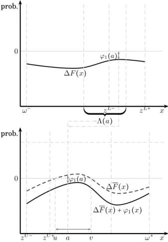
[Insert Figure 3 here.]
Figure 3 illustrates Proposition 7. The upper part illustrates the first step of the pro-cedure. The curve plots the difference FA(x) − FB(x) over the maximum “shortfall” illfare domain. Condition (40) is fulfilled since the curve systematically returns negative values over the interval [ω−, zL+]. Both the lower and upper panels are needed for the second step of the procedure. The dashed curve represents the difference FA(x) − FB(x) over the maximum “excess” illfare domain. As condition (40) is respected, ϕ1(x) is non-positive and condition (41) will necessarily be satisfied when the dashed curve is below the horizontal line. So, condition (41) could possibly not be respected when the dashed curve is above the horizontal lines, that is for values of x∈ (u,v). Then for each value a within this in-terval, we first look at the corresponding interval Λ(a) in the “shortfall” illfare domain and consider the values of FA(x) − FB(x) for each value within Λ(a). The largest value corresponds to ϕ1(a) and is added to F
A
(x) − FB
(x) in the lower panel. The continuous black curve in the lower part of Figure 3 thus plots FA(x) − FB(x) + ϕ1(x) for each value within the maximum “excess” illfare domain and it can be seen that condition (41) is ful-filled since the curve is always below the zero horizontal line. Therefore we conclude that there is more illfare in distribution B than in distribution A, according to any members of
˜
Π1(zL+, zU−).
We now illustrate the proposed algorithm with a simple example. Let(ω−, zL−, zL+, zU−, zU+, ω+) = (0,8,10,15,20, 30), A = (3,9,12,12,12, 12, 17,18), and B = (1,1,2,8,12,12, 16, 24). We can
ob-serve that condition (11) is fulfilled ∀x ∈ [0,10], but (12) does not hold for x ∈]16,17] so that Proposition 1 does not hold. Since condition (21) is met (Proposition 3a can thus be applied), it is worth considering condition (41). As FA(x) − FB(x) > 0 only for x ∈]16,17] it is not necessary compute ϕ1(x) for values outside this interval. For values of x within ]16,17] it can be checked that we have to look for the highest value of FA(x)−FB(x) within ⋃x∈]16,17]Λ(x) = Λ(17) = [6,10[. We then find (F
A
(17) − FB
(17)) + ϕ1(17) = 18−28 < 0. Condi-tion (41) is thereby satisfied since ∆F(x) + ϕ1(x) ⩽ 0 ∀x ∈]15,30]. Hence we can argue that illfare in population A is never above B according to any illfare index from ˜Π1(zL+, zU−) and pair of deprivation lines within the subset[8,10] × [15,20].
Finally, note that the power of Propositions 7 and 8 depends heavily on the chosen values for the minimum and maximum deprivation lines. In particular, as the probability
of satisfying condition (41) depends on the width of Λ(x), the ordering power of the two propositions should decrease as the ranges for zL and zU increase. For instance, in our last example, we observed Λ(21) = [2,9] for zL∈ [8,10] and zU ∈ [15,20]. With zL∈ [9,10] and zU ∈ [15,17], Λ(21) would have shrunk to [3,6], effectively decreasing the probability of obtaining FA(21) − FB(21) + ϕ1(21) > 0.
4
Statistical inference
In empirical applications we estimate the following discrete counterpart of equation (4): P(zL, zU) = 1 N N ∑ n=1 π(xn, zL, zU), (48) where N is the sample size and xn is the value of x for individual n. Now, generally the functions π are likely to be different for “shortfall” and “excess” illfare, just as in the example of (6). Hence we can write equation (48) as the sum of two distinct functions π, each multiplied by illfare identification functions:
P(zL, zU) = 1 N N ∑ n=1[π(x n, zL, zU)I(xn⩽ zL)] + 1 N N ∑ n=1[π(x n, zL, zU)I(xn⩾ zU)], (49) where I(test) is an identification function returning 1 if test is fulfilled and 0 otherwise. Now the standard error corresponding to expression (49) of P is going to depend on the standard errors of the two averages on the right-hand side, i.e. ˆσLand ˆσU, plus a negative covariance term. This covariance is negative because whenever xn ⩽ zLthen it is not the case that xn⩾ zU, and vice-versa. After some straightforward manipulations the variance of P is thus: V(P) = σˆ 2 L+ ˆσU2 − 2PLPU N , (50) where: PL∶= 1 N N ∑ n=1[π(x n, zL, zU)I(xn⩽ zL)], (51) PU ∶= 1 N N ∑ n=1[π(x n, zL, zU)I(xn⩾ zU)], (52) ˆ σ2L∶= 1 N ( N ∑ n=1 π(xn, zL, zU)2I(xn⩽ zL)) − PL2, (53) ˆ σU2 ∶= 1 N ( N ∑ n=1 π(xn, zL, zU)2I(xn⩾ zU)) − PU2. (54) The formulas can easily be adjusted to account for complex survey design (see for in-stance Deaton, 1997).
In order to test the stochastic dominance conditions derived above, we follow the testing procedures proposed in Kaur et al. (1994), Davidson and Duclos (2000) and Davidson and Duclos (2012) since they are based on rival hypotheses that make it possible to conclude in a statistically robust manner whether a distribution dominates another one for a given
order of dominance. Basically, the test consists in a first step to oppose for each value of x within the illfare domain the following hypothesis:
⎧⎪⎪⎪ ⎨⎪⎪⎪ ⎩ H0∶ ∆S(x) = 0, H1∶ ∆S(x) < 0. (55) where ∆S(x) is the considered criterion, for instance ∆S(x) = FA(x) − FB(x) in the case of condition (11) in Proposition 1. Non-dominance of distribution A over distribution B occurs when H0 cannot be rejected. Since the functions used for the dominance criteria are basically linear combinations of averages, the hypotheses can be tested using a simple two-sample test. Since the test has to be performed over the whole illfare domain, it can be concluded that distribution A dominates distribution B in a statistically significant manner if H0is rejected for each value of x within the illfare domain at the chosen level of significance. The test statistics for the whole procedure suggested by Kaur et al. (1994) is consequently: tmax= max⎧⎪⎪⎪⎨⎪⎪⎪ ⎩ ∆ ˆS(x) √ ˆ V(SA(x)) + ˆV (SB(x)) RRRRR RRRRR RRRRx∈ [ω −, zL+] ∪ [zU−, ω+]⎫⎪⎪⎪ ⎬⎪⎪⎪ ⎭ (56) where V(SA(x)) is the variance of SA(x). Dominance is thus observed if t
maxis less than the critical value of the standardized normal distribution corresponding to the chosen level of significance.
In spite of its appeal, the procedure is empirically not tractable unless distributions are censored at their tails as noted by Davidson and Duclos (2012). Indeed most observed dis-tributions are likely to show F(ω−) = 0 or F(ω+) = 0 which yields ∆S(x) = 0. In that case, estimating tmax systematically results in the non-rejection of H0. As shown by Davidson and Duclos (2012) for first order dominance tests, while censoring may a priori be at odds with the core axiomatic framework of poverty measurement, especially the strong ver-sions of MON, there are valuable reasons for performing such censoring. From a practical point of view, censoring may be necessary as stochastic dominance procedures are highly sensitive to the presence of outliers: small measurement errors at the tails of the distribu-tion may yield a non-dominance result though dominance should objectively be concluded. From an ethical point of view, it can be said that there are some thresholds at the two tails of Ω under and above which deprivation is total. For instance, consider two overweight persons with severe mobility impairment thereby exhibiting limited social interaction and high risk of premature death. If these two individuals are plainly identical except that the first one is 5kg lighter than the second one, hence resulting in a lower value of the BMI, we could reasonably argue that the BMI difference is not worth reflecting into even a marginal difference with respect to their individual poverty evaluation. Such individu-als ought not to be dropped from the compared sample but to be treated as if they were exactly at the corresponding threshold of complete deprivation.
Censoring is thus a statistical necessity for Kaur et al.’s (1994) testing approach when the information regarding the tails of the observed distribution is limited. However, it is worth stressing that it may conflict with the transfer axiom as it induces non-convexities
of π at the censoring thresholds. Instead of having to choose between statistical robustness and the transfer axiom, it is possible to adopt a lexicographic approach and assume that the arguments in favour of censoring prevails over those that support the transfer axiom. In other words, we can presume that axiom TRA holds only for a limited part of the illfare domain. Indeed, regarding “loss” (“excess”) illfare, if deprivation is total below (above) some threshold cL ∈]ω−, zL[ (cL∈]zU, ω+[), we will thus assume that progressive transfers only have an illfare decreasing effect if the two pre-transfer values of the attribute are within the interval [cL, zL] ([zU, cU]). This is equivalent as defining the transfer axiom with respect to gaps (as in Lambert and Zoli, 2012, for instance) and assume that gap functions reach an upper limit at the censoring threshold.
Although that position is debatable from an ethical point of view, in practice restricted dominance procedures only entail a light censoring. Davidson (2009), for instance, indi-cates that, for restricted dominance procedures at any order to be performed, one only needs to censor the smallest and largest values of the joint sample of the two distribu-tions to be compared. So, in practice, censoring means a very light infringement on the traditional axiomatic framework.
5
Empirical illustration: Child health poverty in Bangladesh,
Colombia and Egypt
5.1 Data and estimation details
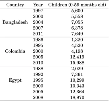
We compute poverty measures for weight-for-age of children (0 to 59 months old) in Bangladesh, Colombia, and Egypt; three large developing countries in South Asia, Latin America, and North Africa. The datasets are: the Bangladesh Demographic and Health Surveys (DHS) for 1997, 2000, 2004 and 2007; the Colombia DHS for 1986, 1995, 2000, 2005 and 2010; and the Egypt DHS for 1988, 1992, 1995, 2000, 2005 and 2008. The DHS have detailed health and anthropometric information for women in child-bearing age and their children, but not for men. Our illustration focuses on under-five children taking advantage of the fact that the range of biologically plausible values for most child health indicators has been defined by the World Health Organization (WHO). Table 1 shows the respective sample sizes for the three countries’ datasets. The computations were performed using household weights and accounting for the clustered and stratified sampling design. Some surveys, e.g. the Bangladesh 2007 DHS, do not have an explicit strata variable, but we generated it as the interaction between region and urban/rural area because that is how strata were defined in other surveys.
[Insert Table 1 here.]
Our illfare evaluations of children rely on the z-scores of weight-for-age, which are com-puted using the WHO software (available at: http://www.who.int/childgrowth/software/en/ (2011)). The underweight and overweight lines are -2 and 2, corresponding to moderate underweight and moderate overweight. The weight-for-age values for ω− and ω+, respec-tively -6 and 5, are taken from the WHO, which regards them as biologically implausible (see http://www.who.int/childgrowth/software/readme_stata.pdf).
We did not estimate other available anthropometric indicators for children due to con-ceptual problems. For instance, while a low height-for-age may reflect malnutrition, a very high height-for-age does not reflect problems attributable to the family or economic environment. Rather it may reflect rare, if potentially detrimental, genetic endowments. Weight-for-height and BMI are not good indicators of health wellbeing among children because a badly malnourished child may be both too short and too thin for his/her age, thereby potentially attaining a deceitfully healthy value for indicators of weight by height.
5.2 Estimation results
5.2.1 Bangladesh
[Insert Table 2 here.]
Table 2 shows the illfare estimates for Bangldeshi children using weight-for-age and members of the FGT family (equation 6) assuming an equal weight for “shortfall” and “ex-cess” forms of illfare (i.e. β = 1). The top third shows headcount indices, i.e. FGT1,0,0. The results show a steady decrease in total illfare in Bangladesh between 1997 and 2011, which relents between 2000 and 2007. The decrease is led by a parallel decrease in “shortfall” illfare that is consistent with the results obtained by Stevens et al. (2012). By contrast, “excess” illfare has first decreased (between 1997 and 2000) and then increased (between 2000 and 2011) during the same period. These observations are consistent with Shafilque et al. (2007) that showed that Bangladesh experienced the same nutrition transition as the majority of developing countries; namely, the coexistence of both decreasing undernu-trition and increasing obesity. The overall result exhibits improvement since “shortfall” illfare in Bangladesh is a more prevalent problem among children. Indeed, Table 3 shows that undernourishment explains at least 99% of the overall headcount index. Thereupon the low values for “excess” illfare using F GT1,1,1and F GT1,2,2are unsurprising (see bottom two-thirds of Table 2 and respective contributions in Table 3).
[Insert Table 3 here.]
Both F GT1,1,1 and F GT1,2,2 have decreased for “shortfall” illfare among children (bot-tom two-thirds of middle column in Table 2). Hence, given the small contributions for “ex-cess” illfare, the period 1997–2011 has witnessed improvement in the intensity of health-related poverty among children in Bangladesh.
5.2.2 Colombia
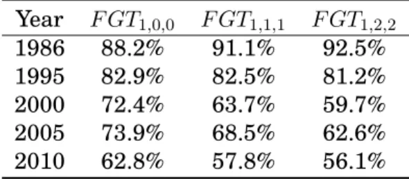
[Insert Table 4 here.] [Insert Table 5 here.]
Table 4 shows the respective illfare estimates for Colombian children. The headcount results show a steady decrease in total illfare in Colombia between 1986 and 2010, without relenting. Compared to Bangladesh, this decrease starts from a lower base of total illfare in their respective initial accounting periods. The decrease is led by a parallel decrease in
“shortfall” illfare. By contrast, “excess” illfare has increased during the same period (albeit with a lull from 2000 to 2005). The overall result exhibits improvement since “shortfall” illfare in Colombia is also relatively a more prevalent problem among children. Indeed, Ta-ble 5 shows that undernourishment explains at least 60% of the overall headcount index. Thereupon the low values for “excess” illfare using F GT1,1,1and F GT1,2,2are unsurprising (see bottom two-thirds of Table 4 and respective contributions in Table 5).
Both F GT1,1,1 and F GT1,2,2 have decreased for “shortfall” illfare among children (bot-tom two-thirds of middle column in Table 4), whereas the same indices show no distinct pattern for “excess” illfare (bottom two-thirds of rightmost column in Table 4). In both cases, of “shortfall” and “excess”, the gaps and square gaps tend to be small, in particular the “shortfall” gaps in Colombia are much smaller than in Bangladesh, signalling a dis-tribution with fewer extreme observations. As for “excess” illfare gaps, while small, their contribution toward total illfare measures has increased throughout the years (two right-most columns in Table 5). Still the “excess” contribution is below 50%, which helps explain why the steady reduction “shortfall” gaps and squared gaps brought about corresponding reductions in the intensity of overall health-related illfare among children in Colombia during the period 1986-2010.
5.2.3 Egypt
[Insert Table 6 here.] [Insert Table 7 here.]
Table 6 shows the illfare estimates for Egyptian children. Unlike the previous cases of Bangladesh and Colombia, Egypt’s headcount results do not show a steady decrease trend in total illfare during the 1988-2008 period. The headcount fluctuates: first increases, then decreases during the 1990s and then goes up again during the last decade. These fluctua-tions in total illfare are not perfectly matched by similar behaviours in either “shortfall” or “excess” illfare, because the two components move in opposite directions between 1988 and 2000. By contrast, from 2000 onward the two measures are synchronized: both increase leading to a corresponding increase in the total illfare headcount. By 2008, total illfare in Egypt is slightly below the 1988 level, mainly due to a net decline in “shortfall” illfare, whereas “excess” illfare exhibits a net increase at the end.
The fluctuating patterns in the headcount are also reflected for both forms of illfare in their respective F GT1,1,1 and F GT1,2,2 measures (bottom two-thirds of middle column in Table 6). In general the “shortfall” gaps and squared gaps of Egypt are between those of Bangladesh and Colombia; whereas the “excess” gaps in Egypt tend to be the high-est among the three countries (with Bangladesh featuring the lowhigh-est “excess” gaps and squared gaps). From 2000 F GT1,1,1 increased steadily in Egypt, due to parallel increases in both “shortfall” and “excess” gaps. Between the two end-points, 1988 and 2008, the in-tensity of “shortfall” illfare experienced a net decrease in Egypt, whereas “excess” illfare moved in the opposite direction.
As a consequence of these trends, the relative importance of “shortfall” illfare among Egyptian children has declined substantially, in terms of the three F GT indices in Table 7).