Approximate state estimation.

RALPH DAVID MASIELLO

SUBMITTED IN PARTIAL FULFILLMENT OF THE REQUIREMENTS FOR THE DEGREES OF

MASTER OF SCIENCE and BACHELOR OF SCIENCE

at the

MASSACHUSETTS INSTITUTE OF TECHNOLOGY August, 1969

Signature of Author

Signature redacted

Department of Electr'cal Eng neering, August 27. 1969 Certified by

Signature redacted

/y' / / sis Supervisor/7

Accepted by

Signature redacted

Chairman, apartmeial'C'mbittee on Graduate Students

Archives

VAss. ISsr. Ec

NOV 12 1969

RALPH DAVID MASIELLO

Submitted to Department of Electrical Engineering on August 27, 1969 in partial fulfillment of the requirements for the Degrees of Master of Science

and Bachelor of Science

ABSTRACT

Simulations have shown the applicability of state estimation techniques to power system control. However, computational

diffi-culties arise in the iteration equation, specifically with regard to the evaluation of a Jacobian matrix and a gain matrix at each iteration.

Using non-linear Fischer estimation theory, modifications are suggested to the Newton's method solution. Approximations are made to the Jacobian matrix and tested satisfactorily. Use of a fixed gain matrix evaluated at system scheduled powers throughout the

iterative sequence is successful, and that gain matrix is successfully approximated before and indicated inversion by zeroing off-diagonal sub-matrices.

The static state estimator is extended to a quasi-static case in which it performs one iteration only for each set of incoming meter readings once it has been started with a first estimate. The ability of the estimator in this mode to track a moving system is tested, and its performance with regard to the errors is described. Its performance is good over a range of values when the system is changing in the form of a ramp change in the scheduled bus powers. This ramp is related to the data rate of a power system metering scheme and some indication of the necessary data rate for tracking is obtained.

The quasi-static state estimator suffers from a tendency to lose the state of the system both randomly throughout what shoald be its operating range and also definitely at the extreme end of that range. Some methods to deal with this problem are suggested and tested, specifically updating the gain matrix and/or the estimate.

Suggestions for further studies are included.

Thesis Supervisor: Fred C. Schweppe Title: Associate Professor of Electrical

of Professor Fred C. Schweppe and was supported in part by the

American Electric Power Service Corporation. All computational

TABLE OF CONTENTS

Introduction: State Estimation and Power Systems 2

1. Preliminaries

A. Power System Equations 5

B. State Estimation 8

C. The Computer Simulation 12

2. Static State Estimation: Approximations to the Jacobian 15 3. Reducing Computation of Sigma

A. Eliminating Evaluation of Sigma at Each Iteration 20

B. Approximating Sigma 26

4. Quasi-Static State Estimation 48

5. Updating Sigma 62

6. Updating the Estimate 65

Eonclusions 78

Suggestions for Further Study 81

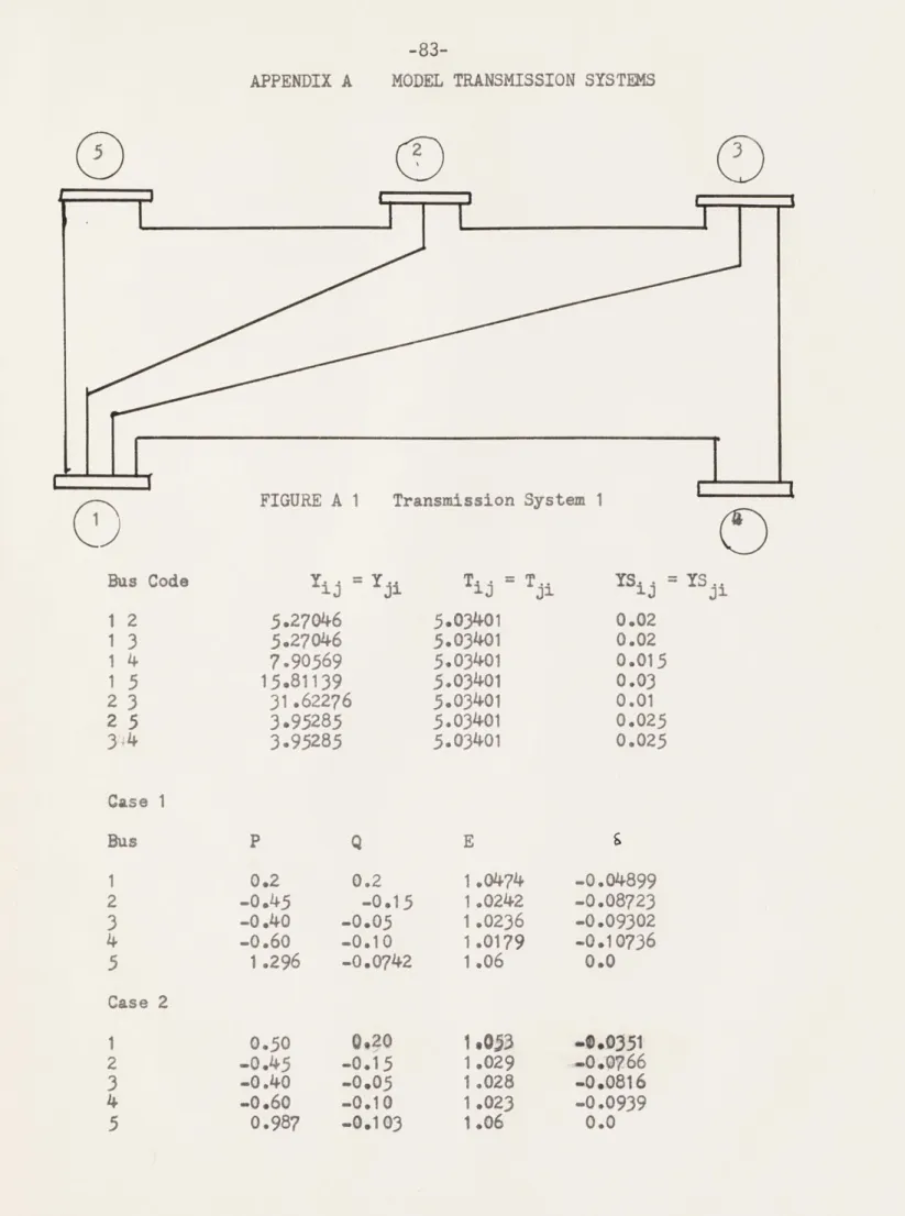
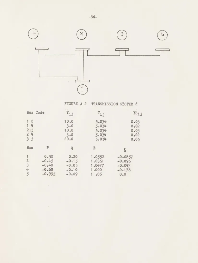
Appendix A: The Model Transmission Systems 83

Appendix B: Computer Flow Charts 86

While the electrical power industry is beginning to use large digital computers as a part of their central control and dispatch systems, the use

made of the larger machines has been primarily to expand existing techniques;

namely load flows and area frequency-power control.

The improved computational ability of the large digital machines makes possible employment of more sophisticated techniques in system observation and control which only recently have been contemplated by the utilities. Work has been done on the application of state estimation techniques to electric utility systems, and the techniques have been shown to be

math-ematically applicab1I and possissed of some advantages in perfomance over

less sophisticated approaches to the problem of system observation.

More specifically, static-state estimation using non-linear Fischer

theory has been applied to computer simulated power systems and the work

has sucessfully extended to include bad data point detection.1,2 The advantage of using a state estimation system is that it makes use of redundant measurements to give an estimate which can be probabil-istically fitted to the structure of the system, or of its mathematical model, such that the expectation of some measure of error is minimized. A state estimator thus accounts for the presence of noise in the input

measurements and can be extended to detect and allow for bad data points. The disadvantage is that due to the non-linear nature of the equations relevant to power systems and due to the large number of variables present the computations are exceedingly complex. So complex, in fact, that a straightforward implementation of state estimation methods is not practical

success with which simulated application of these methods were met are de-scribed. When possible, intrepretation and explanation are offered. The methods, most of which are successive simplifying spproximations, are

presented in the order of thier development with the accompanying logic, if any, at each stage. It is not claimed that sufficient mathematical insight was achieved at the start of the study to show the nature of the final

results, although the goal was defined, albeit loosely, at the start. The work attempts to propose and evaluate some simplifications which hopefully will succeed in removing some of the objections to state

estimat-ion. The mathematical preliminary makes clear the detailed nature of

some of these problems., which briefly are: the evaluation of a large and

complicated Jacobian matrix at each iteration in a sequence which hopefully

converges on the best estimate for the state, the evaluation of an even more complicated gain matrix which requires a matrix invers*on at each step

in the iterative sequence, the storage of that matrix, and the undesirably

large amounts of computer time required to repeat the iterative sequence to

solution of a best estimate corresponding to each of many sets of telemetered meter readings throughout the course of an operating day.

Section 2 discusses approximations to the Jacobian matrix which may

facillitate its evaluation. Section 3 discusses use of a gain matrix

eval-uated at some set of nominal state values corresponding to the system

scheduled values. That gain matrix is then held constant throughout the iterative sequence. A simplification is then presented, namely deleting the off-diagonal sub-matrices of the gain matrix before inversion, which simplifies both evaluation and storage.

estimator to a quasi-dynamic case, that is, attampting to obtain a running estimate of the system state without iterating to convergence for a best

estimate solution at each successive set of input data. Section 4 describes

initial attempts to implement such a scheme, and sections 5 and 6 discuss methods to improve the performance of a quasi-dynamic state estimator. Sections 5 and 6 also present the employment of the simplifying methods developdd on the static case to the quasi-static case.

A. POWER SYSTEM EQUATIONS

In general power systems operate via large magnitudes of voltages, currents, and powers, all of which are time varying (60 cycle A.C.), and all of which are posessed not only of phase angle relative to each other,

but also relative to other locations in the system. A set of equations which is more easily wielded than those derived from straightforward

circuit analysis is obtained using one line diagrams and the per-unit system. The per unit system simply expresses the system during balanced three-phase operation in terms of normalized r.m.s. figures. The system itself is then modelled as a network of real and complex circuit elements operating at voltages which have magnitude and phase. The reader is referred to reference (4) for a detailed description.

The system is modelled as shown in figure 1.1, with the variables defined as follows:

E i Magnitude of voltage at bus i

Phase angle of the voltage at bus i

referred to some bus at which the phase angle is 0 always. P. Real part of complex power entering the system at bus i

Q.

Imaginary part of complex power entering the system at bus i Y Magnitude of the complex series admittance of the line from

bus i to bus

j.

(Note that all lines with both ends at common busses are lumped as one line)

YS.. Magnitude of the imaginary shunt admittance(capacitive)

V= E e

j6

Bus i YB₁ PL

P.,

Q.

T. .=T.. iS. iS. 13 31

YSi

YS i---P. Vl E e Qj Bus

j

YB 3 Q. ivl

Thus Y = Y. eTij

YB Magnitude of the imaginary shunt admittance at bus i. PL Real part of the complex power flowing down the line from

bus i to bus j, as measured at the bus i end of the line. Thus PL. i' PL .

QL Imaginary part of the complex power flow from bus i to bus j as measured at the bus i end of the line.

The definitions for complex power in terms of voltage and current remain unchanged, and lead to the relationships with whith the estimator works.

1.1)

P..

+

jQ..

=

v. '.

1.2) P = IPL

Sj ₁

1.3)

_Q

₌

_ZQL..

1.4) P +

jQ

= VI[(V - V.)Y.. ejTj * or

1.5) PL = ( )2Y cosT - E E Y .cos(T.. + 6 - 6.)

1.6) QL = -(Ei) 2_(YijsinT

1j + YS..) + E.E.Y. sin(T.. + 6.- 6.)

Since the model systems used in the studycontained no shunt admitt-ance at the busses, the terms including YB have been dropped, although the computer coding dnicluded them.

The states of the power system should be a set of variables which uniquely determine all the other measurable variables of the system. The voltage magnitudes and angles will do very well as such a set, and are indeed the most easily handled. While the real and reactive power flows might also uniquely define all the other variables, they are not as easily manipulated. The state vector will always be defined as follows:

EN

6

_N-lj

where N is the number of busses in the system and the Nth bus is always at 0 phase angle. A set of observed values can also be defined,

z = H(xj

where z is made up of observed (metered) voltages, real and reactive bus power flows, and real and reactive line power flows. The vector function H(x) is defined by the power equations (1.1 - 1.6).

These observed values originate from various meters located about the system, telemetering their readings to the central controller. The problem of the state estimator is to obtain from a set of observed values z which are degraded by noise a best estimate of the true state

many models of the system noise and operation, and reflecting several types of probabilistic estimation. The statement which with this study works is as follows:

Given z = zT + v = H_(x)+ v

E[v.] = 0 where v is a random vector assumed

1/

E[(v) = R to be Gaussian with zero mean and

or diagonal covariance R.

E[v.v.'] = R

R will be written as a square matrix with the understanding that it is diagonal for the purposes of this study.

The problem of the estimator is to minimize the cost of the estimate, J, where

J = [(H_(x) - z)' R - z)

If R is diagonal with all non-zero elements equal, then J can be usefully be written as

j = z - H(x)|

Two norms were used in the simulation

J% =1|z - H(x)|l = |zi - Hi (x)|

J=

Iz

- H(x) 2 = (z. - H_(x))

The superscript 1 or 2 will indicate which norm is being referred to at any time.

structure for x has been fromulated. Thus, Fischer as opposed to Bayseian estimation theory is being used.

J is a highly non-linear function of the various state variables.

Consequently, a direct solution for the minimum of J is not available. An iterative solution using Newton's method for the vector case is sought as follows.

1.7)

ji =x +

[H((x)' R_ H H~

ji

(x.j R[

H

H(x)]

where H (x.) is the Jacobian,

-x

-1az.

H(x.)= [h =--- ]

ax.

The iterative process continues until J i+₁ - Ji| is less that some value

which is the convergence criterion.

This is the process which has been used with good results by a

simulated state estimator for power systems. However, the computation is not without its drawbacks.

First, the Jacobian H(x)must be evaluated at each iteration. For the case of voltmeters, z = Ek and the Jacobian contains a fow

j

with zeros everywhere except column k which contains a 1. For a metered bus power, for example, the partial derivatives are more complicated.

zk i _{azk aP.}

ax. ax. .1

Table 2.1 contains a tabulation of the various derivatives. For the case mentioned, if x = E, , 1 i, then

h . = -E.Y cos(T _{+ 6} - 6i)

A glance at table 2.1 shows that the other derivatives are no less compli-cated. The computation of these derivatives adds significantly to the

A far more serious problem in the implementation of the state

estimator is caused by the matrix inversion in the iteration formula. (1.7) This matrix is commonly called the gain matrix, or, here, E.

1.8) E = [H(x)'RH_ (x)]FI

For a'syste m with N busses, the gain matrix (sigma) is of order 2N-l. Performing matrix multiplications and inversions on matrices of this size

( N might typically be between 50 and several hundred) is both difficult

because of round-off error and time consuming because of the large number of computations required. Furthermore, this matrix aggravates a perhaps already serious problem in terms of storage in computer memory. The Jacobian is at least as large as the gain matrix, and the two together may require an undue amount of main memory. While devices to augment

storage beyond that available in main memory are available, all such devices usually slow down computation time to a significant degree.

The inversion is possibly not achievable in a computational sense. While the gain matrix may be non-singular, round-off errors can effectively'

render it either singular or grossly inaccurate, particularly if the matrix is both large and ill-conditioned. This matrix inversion which must be performed at each iteration is one of the major problems in implemetnation of a state estimation scheme for power systems.

Continuous operation of an estimator during the course of an operating day would involve many such inversions if an exact iteration scheme were followed. What is desired, then, is a series of approximations, or compu-tational shortcuts, making implementation iiore realizable.

A computer program similar to ones used in earlier studies of power

system static state estimation1,2 was used as a starting point. Flow charts of the programs used in studies on the static state estimator and as modified for the quasi-static sttte estimator appear in appendix B. Some modifications were made to facillitate forming approximations to the Jacobian and the gain matrix.

The program can be viewed as having three parts: first, a simulation of the power system and associated noisy metering, second, the state est-imator, and third, an evaluation of the performance of the estimator. The program accepts ad data a description of the transmission system and the meters, the values of noise standard deviations (including the deviations of true bus flows from scheduled bus flows), and the

scheduled bus flows for each run.

The estimator is fed the scheduled flows for use in computing an initial guess of the state of the system and for use in computing a nominal gain matrix if that is desired. (including any approximations

which are indicated) True bus powers (real and reactive) are derived by adding noise (a random, Gaussian vector) to the scheduled flows, and the corresponding tnue voltages and angles are found. This provides the true state and the true observation vector. The observation vector provided to the estimator as the readings of simulated meters is the

true observation vector corrupted by noise. The noise added to the

observation vector can be added in one of two ways. Either

z = ZTi +v. or z = zTi X( l + vi)

however, which type of noise was used in any particular trial will be indicated. It should be noted that the program accepts as noise input the standard deviation of the appropriate random variable, so that the actual noise standard deviation in the multiplicative case is not the standard deviation supplied as input, but rather is the input value multiplied by the appropriate observation value. As the estimator used the input value for the standard deviation in any case as the value for the diagonal of R, this implies a non-optimal gain sequence and gain matrix insofar as the noise is concdrned. However, this choice was felt to be reasonable as no data is available on the actual nature of noise to be encountered, so that a certain amount of non-optimal guesses regarding the noise is inevitable. Also, the studies were run with values such that the observation vectors had components not too far removed in magnitude from 1, so that the non-optimality here is not

so great. Later studies were made with appropriate corrections in R to

account for this.

The estimator is also supplied with a convergence criterion and a

maximum number of iterations to be made in any given attempt to find a

minimum value of J. Thus it is possible for the estimator to converge,

fail to converge in the maximum number of allowed iterations, or to diverge on any given trial. By divergence it is meant that the value of J grows with each iteration beyond a specified large value, such as 105

The part of the program which evaluated estimator performance

computes various absolute and percentage errors assocaited with estimate of the state, observation, and bus variables. As this study was not

schemes but rather with the convergence performance of those schemes, the errors are not heavily recorded or intrepreted here.

The author feels that the Jacobian as it appears in the iteration sequence seperately from the gain matrix must be evaluated to a fair degree of accuracy if the iteration sequence is to converge. It is true that good results have been obtained by linearizing the power equations which deal with real power.3 (1.2,1.4,1.5) This operates, in a sense, in the way that a gross simplification to the Jacobian would. However, these results were obtained only when the X/R ratio of the power system was fairly high. (That is to say, the system was relatively lossless)

Also, the reactive powers are not as likely to produce good results with this method. (As T₁j approaches -900, the cos term in eqn. 1.5 can be

linearized about the difference in bus phase angles. However, the sin term in eqn. 1.6 for QL will not yield as readily to such a method)

Some approximations, can, however, be made. Referring to Table 2.1, the value of h.. when z. is PLk, and x is 61 (2.1.11) appears identical to a term appearing in eqn. (1.6) for QLkl. Similar results occur with all the partial derivatives with respect to phase angles. It is not necessary, then, to compute these terms in the Jacobian separately, but rather it is sufficient to use terms in the computation of H(x) as they are computed, and simultaneously store these terms in the Jacobian.

A similar pro cedure can be carried out with the partial derivatives

with respect to bus voltages, after some thought. These derivatives

will have the units of power/voltage, as the voltage with which the derivative is being carried out will decrease in exponential power. Power systems are operated with the per unit voltage at any given bus

ELEMENTS OF THE JACOBIAN

z x _{h i}

Pk El, 1k -Ekcos(Tkl + 61 - 6k)Ykl 2.1.1

E E ₆

cs

k 1kYkl[2_{EkcosTkl - E cos(Tkl + 61 k) 2.1.2}

P , 1jk EkElYklsin(Tkl + 6d - 6k) 2.1.3

Pk 6k -EkE Yklsin(Tkl + 61 - 6k) 2.1.4

Qk El , k Ek klsin(Tkl + 6 - 6k) 2.1.5

k Ek -2Ek[YklsinTkl +YSkl] +EIYklsin(Tkl +

6i - 6k) 2.1.6

Qk 6 , 1tk EkE Yklcos(Tkl + 6i - 6k) 2.1.7

Qk 6k z -EkE Yklcos(Tkl + 6i - 6k) 2.1.8

PLkl E1 , -Ekcos(Tkl + 61 - 6 k)Yl 2.1.9

PLkl Ek Ykl[2_{EkcosTkl - Elcos(Tkl +} 6 _- 6_{k) 2.1.10}

PLkl 61 EkE1Yklsin(Tkl + 6 - 6k) 2.1.11

PLkl 6k -EkE Yklsin(Tkl + 6 - 6k) 2.1.12

QLkl E1 Ek Yklsin(Tkl + 61 - 6k) 2.1.13

QLkl _{Ek -}2_Ek[YklsinTkl

+YSk1l _{+El Yklsin(Tkl +}

61 - 6k) 2.1.14

QLkl 6 EkEIYklcos(Tkl + 6 1 - 6k) 2.1.15

QLkl 6k -EkE Yklcos(Tkl + 6 1 - 6k) 2.1.16

Ek Ek

per unit might be reasonable. Thus the derivatives can be approximated

by ignoring the factor of EkI or E1I as the case may be. Then the

derivatives with respect to voltage would be identical to terms ocurring in the evaluation of line and bus powers. It then is only necessary to store appropriate terms or sums of terms in the power computations in the Jacobian in the appropriate locations. A tabulation of the approximations

made appears in table 2.2 .

Some small saving is achieved by using existing terms; unfortunately, these savings can be achieved only by clever programming and are at best small. A state estimator was tested using these approximations to the

derivatives. Rather than present large amounts of data, I will state

that the performance of the estimator at moderate noise (v. = up to 0.1)

was nearly indistinguishable from that achieved when an exact Jacobian was employed. The approximate Jacobian was used in all further studies, and was extensively used in loadflows make for these studies. A test

performed on loadflows produced the same results with exact and approximate Jacobians within the tolerance of roundoff error. The roundoff error

entered into the picture as the two programs performed sums and

multiplic-ations in different orders. The model system and test case used appear

in fig. 1, appendix A. Table 2.3 shows the number of iterations to

convergence for some trials of the estimator using the approximtte Jacobian. In the future, the Jacobian will be written as before, with the understanding that the approximate Jacobian was used and is being referred to.

Table 2.3 shows trials which used a different convergence criteria from that used by Wilde.1 Consequently, direct comparisons are not available. However, when this was discovered, sufficient confidence had been obtained

TABLE 2.2

APPROXIMATE ELEMENTS OF THE JACOBIAN

z x h i(as approximated)

Pk E 1 , lk -EkEIYklcos(Tkl + 6 1 -6k) 2.2.1

P k E k EEk1Ek Ykl[2EkcosTkl - EIcos(Tkl + 61 - 6k) 2.2.2

Qk E , 10k EkE1Yklsin(Tkl + 61 - 6k) 2.2.3

Ek Z-2E 2 [YklsinTkl + YSk +EkElYksin(

Tkl + 61 - 6k) 2.2.4

PLkl EI -EkEIYklcos(Tkl + 6i - 6k) 2.2.5

PLkl Ek kykl[2_{Ekcos(T kl) -EIcosTkl + 6 - 6k) 2.2.6}

QLkl EI EkE1Yklsin(Tkl + 61 - 6k) 2.2.7

QLkl Ek E2[-2YklsinTkl YSk) + EkElYklsin(

TABLE 2..3

ITERATIONS TO CONVERGENCE USING APPROXIMATE JACOBIAN

Meters

E(5),P(1,2,3,4), Q(1,2,3,4) E(), P(0,2; 1,3; 1,4; 1,5), QL(1,2; 1,3; 1,4; 1,5) Noise Standard Deviation 0.02 multiplicative 0.05 multiplicative 0.10 " 0.20 0.02 0.05 0.10 0.20 multiplicative " "s " Iterations to Convergence of trials 1,1,1,2,1,1 2,2,2,2,2,2 2,2,2,3,2,2

6,3,(divergence caused run to end)

2,2,2,2,2,2 2,3,2,2,3,2 2,2,3,3,2,3 6,3,4,9,4,2 E(1,2,3,5), 0.02 multiplicative 2,1,2,2,2,2 P(1,2,3,5), Q(1,2,3,5) 0.05 " 2,2,2,2,2,2 0.10 " 03,2,2,3,3 0.20 3,3,3,3,5,3

The convergence criterion for these trials was that

2 jf < 10-4

The initial guess of the estimator in each case was the scheduled values supplied to the program; true values were the scheduled values plus noise of the same type and standard deviation as applied to the meter observations.

3 A REDUCING COMPUTATION OF SIGMA

ELIMINATING EVALUATION OF SIGMA AT EACH ITERATION The first logical step in reducing computation time due to the gain matrix was to see if the state estimator would converge using a fixed

sigma at some nominal values. Consequently, the estimator was modified to evalueate sigma at some scheduled values before the start of a series of trials and then to use this sigma for all iterations. Trials were made first adding noise only to the observations, that is, letting the

true bus flow values equal the scheduled values. When this proved successful the true values were set equal to the scheduled values plus noise. Table 3.1 shows results obtained with these methods. Errors are not presented as they were whit would hae been expected had sigma been

constantly re-evaluated. The consideration here is that it was important to determine whether convergence could be obtained, and success with one simplification usually precluded another simplification.

As the value of the nose proceeded towards 0.20, the performance of the estimator became less reliable. However, noise levels may not be expected to be as large as 0.10 so that this performance is acceptable. The number of iterations required tends to increase with increasing

noise and increasing number of approximations and simplifications.

A measure of just how far sigma can get from the exact sigma

can be obtained to an order of magnitude as follows.

- x H ( R 1 Hx (x)

A sensitivity of terms in scheduled vs. exact sigma for changes in

true flows and states from scheduled can be achieved un light of the approximations to the Jacobian which can be regarded as powers.

-l

0 a . 0 0 0 0

13

0 a2j 0 ajl aj2 j3 ajn

= a3j

lnj

0 0 0

a

ni

so that _Dakl

as

= -aki~jI 3.1

As an example, consider the following elements chosen from the matrices in fig. 3.1 .

- =- -32 = 0.025 x 0.03 = 7.5 x 10-5

What is s28 ?

s= Zhxkr hxk

k ki k k

k rk- azk 3Z k

ax _ax.

This sum has non-zero terms only when z k is a measurement of some voltage, bus power, or line power, made at some bus m such that Y. , Y j $ or if i=m or if j=m. If, for instance, zk = i, then an order of magnitude for this sum might be P.QR~i . If a deviation of true flows of 0.02 standard deviation, this deviation will roughly be

P+ A term of the magnitude PiQi represents derivatives with

50 R

respect to variables both at that bus - i.e., it is the largest such term likely. Call P. = 0.5, Q. = 0.3, then s.. is roughly 50. The corresponding term in fig. 3.J is closer to 500, due to the fact that derivatives are often larger than the terms they represent by an order of magnitude. This is because terms of nearly the same magnitude but of opposite sign are added to get any given line power flow. The derivation destroys this balance.

For the values hypothesized, ds would be between 1 and 10. Then a total change in the inverse dc = 7.5 x 10 -. But this is for a noise level of 0.02, when things workd well. At ten percent noise (0.10) this sensitivity will increase by a factor of 5. At this level, the change in the term of the inverse is nearly the same order of magnitude as the original term was. These numbers are crude approximations

but they indicate how it is that a seemingly small change in the true states can cause a significant change in the exact sigma matrix.

TABLE 3.1

FIXED SIGMA EVALUATED AT SCHEDULED VALUES

1.) True values of bus power flows = scheduled values

Meters

Noise Iterations to convergence

E(5), P(1,2,3,4), Q (1,2,3,4) E(1,2,3,5), P(1,2,3,5), Q(1 ,2,3,5) 0.02 multiplicative 0.05 0.10 " " 0.02 multiplicative 0.05 0.10 0.20 i I "I 2,2,2,2,2,2 2,322,2,3,2

2,3, divergence caused run to end

2,2,2,2,2,2 2,292,2,2,2 2,3,3,3,3,2 4,2,3,4, divergence as above E(5), PL(1,2; 1,3; 1,4; 1,5),

QL(1,2; 1,3;

1,4; 1,5) 0.02 multiplicative 0.05 0.10 " " 2,2,2,2,3,2 2,3,3,2,2,3 3,2, divergence as above

The initial guess was the scheduled state of the system, which in

this case co-incided with the true state. The convergence criteria was that | - < 10-4

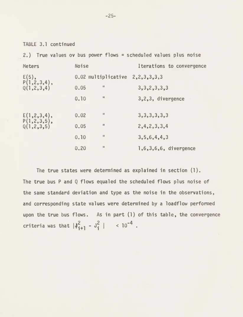
TABLE 3.1 continued

2.) True values ov bus power flows = scheduled values plus noise

Meters Noise Iterations to convergence

E(5), 0.02 multiplicative 2,2,3,3,3,3 P(1,2,3,4), Q(1,2,3,4) 0.05 3,3,2,3,3,3 0.10 3,2,3, divergence E(1,2,3,4), 0.02 3,3,3,3,3,3 P(1,2,3,5), Q(1,2,3,5) 0.05 2,4,2,3,3,4 0.10 3,5,6,4,4,3 0.20 1,6,3,6,6, divergence

The true states were determined as explained in section (1). The true bus P and

Q

flows equaled the scheduled flows plus noise of the same standard deviation and type as the noise in the observations, and corresponding state values were determined by a loadflow performed upon the true bus flows. As in part (1) of this table, the convergence criteria was that | 1 2 <1

3 B APPROXIMATING SIGMA

While it may not be necessary to invert the gain matrix at each iteration, it is still necessary to perform the indicated inversion at least once for each series of estimation about a given set of

scheduled values, and to store the resulting matrix. Even if the matrix is assumed to be sparce to the extent that 80% of the elements are zero, a considerable amount of storage is required.

Consequently, a method is desired which will reduce storage require-metns and computation time due to inversion while still providing

reasonable performance. Several methods were attempted, based on experienced suggestion, on a basis of what would be a reasonable expectation of behavior, or based on what would be desired behavior. Also, sevdral theoretical considerations were held in mind. The

coupling between variables at the same bus is stronger tha that between variables at busses which are electrically distnant. For systems with a moderately high X/R ratio, it is possible to separate voltage and angle to some extent.

So that any indication of success would be noticed, the various methods were tested under extremely favorabel conditions: the value

of the noise standard deviations was 0.01 both for the true versus scheduled bus flows and for the observed versus true meter readings. The initial guess was always the scheduled values.

Some of the methods which were tried are listed, along with comments as to results and causes of success or a lack of it.

1.) Diagonalizing sigma after the inversion had been performed. This method consistently led to quick divergence of the estimate.

2.) Setting the off-diagonal sub-matrices to zero. This was done after the inversion had been performed. While this method did not lead to consistent divergence, none of the estimates converged within the criteria. (which was that

|I! +

j1

< 10-3. ) Rather, the estimate tended

to oscillate with too large a change in state or

J.

at each iteration for convergence.

1

3.) Zeroing selected elements in the matrix before the inversion had been performed. What was attempted was to zero elements which were smaller than the largest element in their row or column by some

factor. A factbr of 50 produced convergence roughly half the time. Unforutunately, this method did not produce an organized reductionof the matrix, so that its usefulness was decreased.

for intensive testing.

5.) Diagonalizing the matrix before inversion. This method produced sporadic convergence. It was not pursued as the other method has by then proved successful.

The successful method, hereafter called pre-inversion block-diag-onalization, or just block-diagblock-diag-onalization, was tested intensively. Results are tabulated on the following pages, and the following figures are some examples of the gain matrices obtained. The number of iterations required to convergence tends to be higher than in previous trials, which is due to the fact that the convergence criteria was changed to match Wilde'sI so that a check could be made on the errors in the estimate. It is worth noting that the trials at higher noise levels which failed to converge all did so in an oscillatory sense - that is, the value of JI at each iteration was more or less cycling between one of two values

which were too separated for convergence. Had the convergence criteria

been larger (perhaps 10-2 instead of 10~4) these trials would all have converged. A few tests were made with the larger convergence criteria.

These reslts appear in table 3.4. While these few trials are far from

conclusive, it would seem that a larger convergence criteria could be used wihtout undue ill effects.

Examination of the sample gain matrices presented (figures 3.1

-.3.4) would seem to indicate that the four sub-matrices all are so uniform within themselves that they could each be set to a constant value for all thefr terms. However, an example of the gain matrices for a different model system (figures 3.5- 3.8) will reveal that this is not the case.

Needless to say, this result with the block-diagonalized sigma inverse was surprising. A partial explanation only is offered, and i is somewhat tortuous.

Write dz= [H(x) - z]

Then or

which is

Now examine the i Call Then And if Then But So that _dx = _

H_

(x')' R~ dz -1

d=+1

i I i -x

-x-

)'- -z [H (x)' R~ H (x )

]

dx H(x) R-1 dzi

ndividual terms in (3.4) as sums.

H. (x

) R7' dz = dw1 dw = _{k dzk/ Rk} ax E~1 = [s i] E s.. dx = E az dz

1 U l

k -k dk /Rk

ax.k

_3x s.. =

z az

az

1

m_

a __m /R

ax.

3x

m M zzaz 1 m . . ax

am

dx_{1 3z dzk} x Rm kax.

t

3.2 3.3 3.4 3.5 3.6 3.7 3.8 3. ?

Equation 3.9 is simply an expression for the jth term in equation 3.4 .

Expand the left side of 3.5

[

dx, (

2zi

az + ' ' + az azM /R

ax axL aj x

3.10 (The upper case L is used to make clear that the zi reads z subscript one)

The terms in the left side of (3.9) for l>N, N the number of busses

and j<N are of interest. These correspond to the upper right-hand' sub-matrix of sigma inverse, specifically those terms such that all the azm refer to azm for some p.

At this point it is convenient to introduce as an observation the fact that the spread between the various phase angles at the busses in this model system is not very large, in fact, all the angles are of

roughly the same order of magnitude. (except, of course, the slack bus, which does not enter these equations in any event.) Now, make the

hypothesis that in addition to this fact, the change in estimated angle at anu iteration is roughly the same at each bus. (patently not true, but this can be resolved more pointedly once the consequences are made clear)

Then, for all the dx. where j>N, or where x. is some phase angle, all the dx. can be called the same value,

d

This approximation permits simplification of the left sum in equation 3.10 as follows.

Consider only those L for which xL corresponds to a phase angle. Call these L' . Then

is the same as

Tlis can be rewritten

dxL,

_I

_{azl az} 1 j /R

T6[

az

1

az

1 x ax₁, /R1 ax i1 3.10 0....

]

ai"

by factoring out the azk as follows. ax~

azk

--- k L

k _{ak /Rk}

ax k

Observe the portion

E az k

L _{x L'}

This is a sum over angles ( xL')

Let zk be a bus power, for example. Then, using equations 1.2, 1.5, 2.1.3, and 2.1.4, 3.12 can be written as:

3.11 3.12 p E qYqpsin(T qp+ 6 p 6 )] + aP 36q 3.13 s a

as s

which is E p Eqyqpsin(Tqp + 6 - 6q)

-E E E Y sin(T + 6 - 6 ) 3.14

P qp qp qp p q

but since Y q , 3.14 is uniquely zero. It is not hard to see that this will happen for any zk regardless of what kind of meter it represents.

Thus to the oreder of the approximation that all the dx. where x. is a phase angle are equal, the sum 3.11 is zero. This is equivalent

to saying that the portion of the jth component of 3.4 due to the upper right sub-matrix of the gain matrix is negligible. If this is the case, why not set all those elements to zero? Which, of course, is what the method of block-diagonalization does. Symmetry argues that the same thing be done to the lower left-hand sub=matrix. (Although the corresponding equations have yet to yield to such a result, symmetry or no)

At first it would seem that this method would work only if the approximation that all the dx. for the appropriate

j

were equal. Not only is that assumption clearly not true, but even a rough equality of

the phase angles is only the case if the system is tightly connected as the model is and then only if the slack ious is carefully chosen. That is, a radial sort of symmetry is apparently desired about the

slack bus of the system. Fortunately, this point can be removed as an objection.

xL'

q

Thus the dx. need only be approximately equal at adjoining busses for the desired cancellation to occur.

Now, even if the spread in phase angle across a system is large, that spread will be distributed gradually. Thus the angle difference across any one line should be small compared to the total phase angle spread

if that spread is large. So adjoinging busses will be "close" to each other insofar as phase angle is concerned. Furthermore, if the state estimate of one bus "responds" to a change in true bus flow from scheduled bus flow by increasing or decreasing the phase angle at that bus, it will tend to "pull" adjoining busses with it.

In this sense, then, the dx. where

j

is an L' are equal to the extent required for this explanation to hold.

As a means of verifying this to some extent, the estimator with the block-diagonalized sigma was tested on another model system so chosen as not to be at all tightly connected or radially constructed.

In addition, the slack bus was chosen so as to maximizd the phase angle across the system. This system is system 2 in appendix A.

The results of these studies appear in figures 3.5 - 3.8 and in tables

3.5 and 3.6 . The other tables and figures refer to studies on the

same system as used earlier, although the scheduled bus flows were changed for these trials to accomodate the quasi-static state estimator as will be explained when that part of the work is discussed. The scheduled flows correspond to case 0 in appendix A.

The estimator performed nearly as well on the second system as it did on the first. The larger numbers of iterations to convergence are due more to the fact that iterative changes in bus voltages and phase angles take longer to propogate through the system than because the approximations are less accurate. It is to be expected that this

method will work better as the X/R ratio of the model system increases, as it effectively separates the voltage and angle from each other in the iteration sequence.

PERFORMANCE OF APPROXIMATE SIGMA 1 1* P-h0 0 0.02 22 17 1 9' 13 8 15

3'

94 2 0.05 11 6

5

5

7 13 26 24

9

15

0.10 26 3 4 0. 0. 0 0. 0. 0 0. 0. 0. 0. ' Errors 044 7.9 4.9 016 27 25 .022 _{7.9 11} 026 6.1 4.5 048 .26 9.5 .028 13 15 021 3.3 3.1 011 1.4 _3.9 030 26 1.3 064 .76 10 0.08 0.06 0.05 0.07 0.012 0.02 0.05

0.13

0.04 0.07 0.11 0.11 0.14

53

9.9

8.1 2.9 30 1.4 11 8.4

15

24 $10 3.4 .42 1.2

5

2.3 8.6

3.6

27 26 7.4 6.4 6.5 8.9 X 10- 3 6.7 1.6 1.1

averaged over busses

5.9

5.9

12 4.4 12 1.5

5.6

5.7

10 11 15 29 11 15 12

30

15 23 25 24 If 10-6 2.5 2.8 2.0 6.1 3.8 1.7 1.2 2.2 3.4 1.3 7.6 5.4 l.1L 1.2 2.1 .84 2.1

.3

1.2 1.0 1.0 1.7 13 3.1 8.0 5.1 3.1 2.1 7.4 3.2 4.8 1.2 5.0 5.2 2.7 2.7 21 3.6

9.7

4.1 14 4.6 x /0, z 1.8 10

.5

4.7

1.6 6.3

(only three trials were made at this noise level)

Meters: E(5), P(l,2,3,4), Q(1,2,3,4) Convergence criteria: Ji+

i

1

Initial guess: scheuled values at which sigma was evaluated

Tune bus power flows

=

scheduled bus power flows + noise of the same noise level as the meter noise.

All noise was multiplicative.

1.6

5.7

3.6 1.4 1.3 1.8 3.2 1.2 1.4 4.6 15 8.6 2.8 7.8 4.1 4.4 2.7 23 8.5 14

30

4.5

24

0f C 41 d -I-k 0.02 25 9 14 2 17 13 14 14 7 15 0.02

0.05

0.045 0.07 0.07 0.05 0.02 0*06 0.07 0.06 0.05 12 0.12 34 0.11 19 0.19 10 0.06 5 0.19 2 0.21 four trials 0.10 6 2

35

26 14 18 28 13 0.22 0.36 0.27 0.29 .13

0.3

0.3 0.25

PERFORMANCE OF APPROXIMATE SIGMA

Errors averaged over busses

.83 1 .6 .4 .2 .04 1.40 .07 .03 2.0 .72 4.2 1.5 1.5 .16 3.8 .05 .7 1.7 1.3 .9 .5 1.4 .9 .5 .17 .7 .51 3.7 3.7 2.3 1.2 .13

A-5.3

5.8 11 11 9.0 2.3 11 8.4 18 4.3 11 29 5.1 27 44 24 1.0 1.2 1.8 1.7 1 ,7

.35

1.9 1.2 2.7 .8 29 4.6 0.8 4.7 6.5 4.1 failed to converge in 5.3 5.9 9.2 .2 13 4.6 4.2 2.2 5.4 .68 5.2 5.2 .5 4.5 .1 .9 1.5 4.7 5.5 9.7 6.1 3.4 11 8.1 7.8 12 6.4 5.1 9.1 2.8 1.7 3.2

two t'ials failed to converge

2.1 3.0 1.4 .74 1.8 2.3 2.5 .6 3.3 2.0 1.7

3.4

1 .1 .7 1.4 1.8 2.1 .6 3.4 1,6 Meters: E(5), P(1,2.3,4). Q(1,2,3,4), PL(1,2; 1,3; 1,4; 1,5) QL(1,2; 1,4; 1,3; 1.5)

Convergence criteria: Ji+1 - Jj C. 10 Initial guess: scheduled vaikues

All noise was multiplicative

7.6 9.7 4.2 4.1 6.3 _5.5 5.8 5.4 6.8 7.6 6.3 7.2 35 iterations Ac10n-1 .68 5.4 ."5 4.5 1.4 1.1 1.1 8.4 2.3 20 2.2 25 1.3 2.2 2.4 14

PERFORMANCE OF APPROXIMATE SIGMA Errors averaged over busses

vo -'W .1 .6 .82 .15 1.4 .23 1.4 8.0 .8 .76 12.0 5.0 .04 4.3 3.5 17 .07 .67 2.0 30 .06

.77

.78 11 .18 .11 .11 .04 .16 .08 .21 .16 .05 5.2 2.5 2.7 1.3 2.4 2.2 1.5 7.4 5.4 12 3.3 13 9.5 5.2 11 4.2 2.1 4.6 ic to-" 1.3 9.9 .51 4.7 1.8 5.9 22 4.4 26 Meters were E(5), P(1,2,3,4), Q(1,2,3,4), PL(5,1; 5,2) Noise was multiplicative

Initial guess was the scheduled values Convergence criteria was JJ+ J{\ 10-in2

)(- I-1 AV-.02 21 .07 .83 .22 .02 2C ( ~ .34 .53 .16 .05 1.1 .66 .60 .26 .06 2.6 184 t1 . 0 . .14 1.3 1.5 1.4 .47 .29 5.5 .15 .52 2.0 3.0 .36 4.5 2.7 .22 .05 1.3 2.5 .64 4.0 7.2 Meters were E(5), P(1,2,3,4), Q(1,2,3,4), PL(1,2; 1,3;

QL(1, 2; 1,3; 1,4; 1,5) Noise was multiplicative

Initial guess and convergence as above

1.4; 1,5)# _. Q-) 0

z

(%I

u

-K 0.042 0.1 0.04 .02 2 1

3

.05 7

3

3

.10 2

3

8 .02 2 3 2 .05 3 3 2 )<Ib-%

APPROXIMATE SIGMA ON TRANSMISSION SYSTEM 2 Errors averaged over busses

Q. 01*02 LU ' 2 11 11 13 4 7 8 5 13 14 .68 4.2 .49 .05 2.3 .04 .14 2.1 .23 .13 1.5 1.1 .01 .48 .16 .05 .04 .04 .05 .08 .62 0.7 1.6 .57 .92 1 .1 .91 .92 2.4 1.2 .19 .36 .13 .2 .33 .28 .22 .58 .33 .25 .24 0.6 .56 .11 .36 .2 .39 .14 .61 .44 .7 .12 .32 .11 .06 .07 .02 .16 .13 .18 1.2 1.4 2.5 0.1 1.6 1.6 1.7 1.4 3.7 1.9 3.4 3.6 2.0 3.4 5.1 5.0 3.'.2 8.8 5.2 4.3 2.1 6.1 5.6 0.9 3.5 1.5 3.3 1.2 5.4 3.5 2.7 17 2.9 13 6.4 7.4 2.8 19 14 22 0.17 0.014 .006 .005 .008 .019 .02 .008 .009 .007 .02 .03 .002 .017 .04 .004 .007 .01 .05 .005 .01 .01 .01 Meters: E(5), P(1,2,3,4), Q(1,2,3,4) Noise: multiplicative

Initial guess: scheduled states Convergence criteria: j ;-J 1- 3 .48 .28 .79 .3 12 11 .17 .04 .29 .07 4.4 16 .17 .11 .42 .22 7.1 69 -t'N LWI x .78 2.7 .97 .55 .27 1.7 .06 .19 3.1 .61 .82 .19 .11 .07 .32 .05 .08 .85 .83 .36 0005 26 7 14 7 3 14 5 24 4 26 0.10 25 13 22

APPROXIMATE SIGMA ON TRANSMISSION SYSTEM 2

0 O

Q)

0

Errors averaged over busses LLV 0.02 23 .02 7 .05 5 .07 4 .03 4 .04 11 .03 5 .04 16 .02 6 .09 3 .05 0.05 3 .12 7 .16 5 .07 17 .09 13 .08 5 .07 6 .24 three 0.10 13 8 22

3

8 6 6 7 .27 .15 .18 .22 .09 .46 .34 .25 .82 .12 .08 .07 .06 1.1

.35

.3

1 .2 .72

3.4

.3 -1 .1 3.2 .56 3.0 trials 1.2 1.1 .07

3.5

.63 7.1 .37

3.3

10 .41 1.3 2.3

.36

.19

.9

2.1 388 .4 1.1 4.0 6.3 .92 .49 2.8 5.3 .67 failed .6 .8 .86 .43 .65 .44 .14 .6 .64 1.2 1.8 2.3 1.1 1.6 1.0 3.3 1.9 .15 .2 .15 .11 .18 .17 .2 .17

.37

.44 .49

.54

.27

.39

.46 .4

.75

to converge 1 .1 1.5 1.3 .8 1.3 .6 2.4 .99 1 .0 1.9

3.5

3.2 2.2

3.3

1.4

5.7

2.9 X10-2 1.4 4.2 .82 6.4 .21 2.2 .66 4.4 .10 .32

.95

6.4 .06 3.1 .90 4.9 .91 5.5 .84 10 .17 3.8 1.8 5.9 .23 3.4 1.7 6.6 1.0 8.1 .92 13 0a 1.2 2.3 1.3 1.3 1.8 1.3 2.4 1.8

3.9

1.5

6.5

5.3

3.9

3.7

3.7

5.0

8.7 6.7 6.9 9.0 8.8 5.6 19 17 8.4 two trials failed to converged

Meters: E(5), P(1,2,3,4), Q(1,2,3,4), PL(5,3; 1,2), QL(5,3; 1,2) Noise: multiplicative

Initial .guess : scheduled values

Zo-O

:OSLONj

3

3SV3

6

L W31SAS

NOISSIWSN'dLh

Si03 VWSIS

L*C

W3I9

COSa699

0

Co-z

I690

co-a i

L19o co-a9OCo o zo-ao lego zo0 L+1100

zo0-K9O17

0 z0-:a o1* 0 z0-H479co0 170 170

co

a

LZ6*0

afz0z* 00. CO-a t69's0 co-aw19 co"'go9 0

co-acgr

0 z0o9 .coo ?Ou O~c 00 z0 917c "o z0-a917c* o zo-agzc 0o 17 aL6"0 90 azgtLo 90 act to0' go azttO' CO a966"O co-i L4790

co-5o9o0

co- C~

"o

co-i917w zo' 96z* 0

zo-azc0

zo- 17zc

0

zo- Hczc

0

zo-acoc*

0 170 90 90 Co co a6C6,,o H4C7 L9 0-co-a9oeC 0

co-acgr'

z0a91lz* 0

Co-I9z

"o

zo-gCvo

z0-agc t 0 zo-HK t. 0 170 170 azozo 0-

L

HL

VO-a1tL 1 9 00-zo-agotCo zo-H96Z*O L O'a6oZ* 0 co CO co 170 a266*0 at94,~ 0 0 zO-a 1400 zo-ao~c 0

zo-aLzC

0

zo-agc

to

tO-zt17WO

t.0 9gr 0 t-zgz 0 0L OLz "0 L0oKizcV 0 Co Co co 10 170 H~qg-90 Hooe'Do M9 0-aczt.* 0 K~r17L 0 zo0917 0 z0" 917 0 zo-at 7 zC* 0 zo-aK7 t * 0 Lo 0z~ t0-az~z 0 L0oQ 0z~ t 0-617Z "0 LotaCzo0 z0o 017 0

z0-a9K

*

0

zo-acC&e Z0 17 l*Oo 1O-H IWzO L0-a tgQ0 t o-6trz 0 tI0H947z0

to-aceCo

UOJ.SJOAUL J8J eUJ6L&

zo

zc17/ "o

170 H96 1"0 50 zzztL0 zo-m7c* 0 zo-ac * 0

io-z0O

Lo-CCz

0 Co

az9t

"o

f

170 9L

"0-Co aLio Co zzioo-170 afzi17L"0- CO SC5o-Co a0ogo 170 ae&0 170 a~2170o 50 a IKO

0--0.202E 05 0.939E 04 -.0.902E 04 0.118E 05 0.748E 04 -0.341E 05 -0.428E 04 0.122E 05 0.748E 04 0.187E 05

0.0 0.0 0.0 .0.O 0.0 0.0 0.0 0.0 0.0 0.0 0.0 0.0 0.0 0.0 0.0 0.0 0.0 0.0 0.0 0.0 0.0 0.0 0.0 0.0 0.911E 05 -0.136E 05 -0.136E 05 0.153E 06 -0.117E 05 -0.143E 06 -0.202E 05 0.939E 04 0.0 0.0 -0.117E ₀₅ -0.143E 06 0.1 52E 06 -0.921E 04 0.0 0.0 -0.202E 05 0.939E 04 -0.921E 04 0.125E 05

Sigma after inversion 0.374E -02 0.401 E-02 0.404E-.02 0.409E-02 0.348E-02 0.0 0.0 0.0 0.0 0.401 E-02 0.438E-02 0.441 E-02 0.441 E-02 0.368E-02 0.0 0.0 0.0 0.0 0.404E-02 0.441 E-02 0.444E-02 0.445E-02 0.369E-02 0.0 t 0.0 0.0 0.0 0.409E-02 0.441 E-02 0.445E-02 0.461 E-02 0 .372E-02 0.0 0.0 0.0 0.0 0 .348E-02 0 .368E-02 0.369E-02 0 .372E-02 0.334E-02 0.0 0.0 0.0 0.0 0.0 0.0 0.0 0.0 0.0 0.432E-04 0.575E-04 0.619E-04 0.720E-04 0.0 0.0 0.0 0.0 0.0 0.575E-04 0.1 33E-03 0.136E-03 0.925E-04 0.0 0.0 0.0 0.0 0.0 0.619E-04 0.136E-03 0 .1 46E-03 0.105E-03 0.0 0.0 0.0 0.0 0.0 0.720E-04 0.925E-04 0 .105E-03 0.204E-03 FIGURE 3.2

APPROXIMATE SIGMA FOR TRANSMISSION SYSTEM 1, CASE 2 Noise: 0.02

Meters: E(5), P(1,2,3,4), Q(1,2,3,4)

Zo-o :aSLON 3SVO '1 W3.LSAS NOISSIWSNV8.1 i0d VWIS VC

RnifUj

ZO-a!Rt79 0 ZO-a lC9 zo-a90e0 c0-Hogg *0 co-qz49o co- to,0 c0-agi9r z0-ag90e0 zo-a~cc 0 zo0 zcc 0 zo-azcco0 zo-39 1c0o c0-aceC90o Co-a tog,,0 Co-a69g 0 Co-a 3 , L0 z03z9z* 0 z0-actco0 z0 I Leoo z0- Ittcoo z039g6z 0 co- 90e 0 co- 99? 0 Co-q LKZ0 co-l~ I"o zodm-a I. z0-agct .6 zo-az0* 0 zo-azc vo z0" CLVO zo-ag~co 0 zo-agoco 0 z0-39e* 0 zo-a zz t o

to'-gle L

O to0aIo0* 0 to0 LOZO0 L03a L0ZI,0 103a L6 o Zo-269CO 0 z0- gCC* 0 L0-M Lz"0 Lo 6szl 0 l0'1gw0o zo-a99co 0 zo-aicc 0o z0-a I Leoo zo-a C Vo 0 1.0-a L0ZI0 Ito-6 LW t 0-azIr o. lo39sLZO, t0-390z 0 z0- g9C*0 zo-ztc* 0 z0-a tL C', z03zzctL0 to0 3z L00 to039 LZOO 109 lzo0 L03i. L, LOi9o0 0 UOj.S49AUL J91JR eWBL zoin3Igce0 zo09 ieoO ZO-296Z 0 zo-H K I*o I031t6L .0 toin3eoz 0 L0'39Oz~O tO3a9Ozo0 t o396 too az9V0o fr0 HLZ6"0 az60o 90 at7t"0 W600o 90 HCf47V0 a9CZ0" 0o HK too-st~oZ'o Co a966o0 agg990" CO s00c*0 470 90 90 go Co 96C6o

act

t

v0-aIt 0 470 470 Co S966 0 397 1 0- aczLV0 Co co Co 347Zo 0 ai966o 0 3a:47z 0- 519f?10-3I.zeo al947/0 CO co CO 470 470 9~999 0-5300COO M t VO-acVto a~47'zo 0 Hg1 0 0 zo

ac'trio

fr0

a3loV0

to0 a96to CO atcg~0 50 a zV0 to70 o6o-CO 3zg9o0

Co

azLgo 470 P1 o 0 CO

ogoo

470 H6 1 4*0-470 36C60o '170 309tVO CO H0C90m CO

a47zz0o

-470 acz L" 50 aqzfro 0 50 a0472-470 470 Co Co (96L WL ! EL !'lOlb (96 L !V L !C L !Z' Old 6(tF4C4Z4L)b 4(V4C4Z6L)d

-0.240E 05 0.939E 04 -0.902E -0.478E 05 -0.418E 04 0.122E

0.0 0.0 0.0 0.0 0.0 0.0 0.0 0.0 0.0 0.0 0.0 0.0 05 0.748E 04 0.321E 0.0 0.0 0.0 0.0 0.0 0.0 0.0 0.0 05 0.0 0.998E 05 -0.152E 05 -0.134E 05 -0.238E 05 0.0 -0.152E ₀₅ 0.1 54E 06 -0.143E 06 0.939E 04 0.0 -0.134E 'O. 1 43E 0 .1 54E -0.921 E 05 06 06 04 0.0 .0.238E 05 0.939E 04 -0.921 E 04 0.1 62E 05

Sigma after inversion 0.277E-02 0.290E-02 0. 290E092 0.292E-02 0.271E-02 0.0 0.0 0.0 0.0 0.290E-02 0 .309E-02 0 .309E-.02 0 .306E..02 0.283E-01 0.0 0.0 0.0 0.0 0.290E-02 0.309E-02 0.31 OE-02 0.307E-02 0.283E-02 0.0 0.0 0.0 0.0 0.292E.02 0.306E-02 0.307E-02 0.31 6E-02 0.284E-02 0.0 0.0 0,0 0.0 0.271 E-02 0.283&02 0.283E-02 0.284E-02 0 .270E-02 0.0 0.0 0.0. 0.0 0.0 0.0 0.0 0.0 0.0 0.407E-04 0.544E-04 0.580E-04 0.615E-04 0.0 0.0 0.0 0.0 0.0 0.544E-04 0.123E03 0.1 24E-03 0.7 95E-04 0.0 0.0 0.0 0.0 0.0 0. 580E-.04 0.124E-03 0.133E-03 0.889E-04 0.0 0.0 0.0 0.0 0.0 0.61 5E-04 0.795E-04 0.889E-04 0.157E-03 FIGURE 3.4

APPROXIMATE SIGMA FOR TRANSMISSION SYSTEM 1, CASE 2 Noise: 0.02

Meters: E(5), P(1,2,3,4), Q(l,2,3,4),

PL(1,2; 1,3; 1,4; 1,5),

QL(1,2; 1,3; 1,4; 1,5)

This sigma corresponds to

the one in <figure 3.3

30'0 :MsLO

I

JSVJ *3 W3ISAS N0ISSIWSNVd Noi0 VM9is S*C RMflIJ zLaz9 .0 Zoar t O

zo-azce

0

z0' 09gco 0 zo-a tg~

1~

Zo-a6go

zo-aeC6 *o

zoO * Co ZHl t* 0 Co-az6ze 0 zo0a09 t 0 z0-atr. zO--06 t 0 0 zo-zR L0

Co-

z

IV'0 zo-ag:oo. zo Otrtr 0

CO-a6

U*

0

z0-a I Lzo0 zo-agei 0 zo'-aztrc 0

zo-a~co

0

zo-McgC

0

zo-a tgzo Z0_H09 to0 to 6c~z 0 LO-a tZo0 zo-ac tzo zo-acogo

zo-agcf4

0

to-azqcoo to-a9 LCO0 zo-a69 0 z0ma00tr* 0 LO-ZZ zoo tL02LZZ 0 to-a6i47o 0 UOLS~aAUL IA84P eW6LS zo-aeC6 0 Z0-aO6 1*0 zo-a9"o 0 zo0aegc0 to-a9 Co Lo-af6'ty?' to-a61yZ*o

z0o-atC6

0 zO**artr 0

zo-acgc*

0

t0-a47wzo0 LO-a9Wz 0 L0-a9zW 0

g*o

ae3oz*o-000 Co acg t o

470

affVO-470 attL 100 000 50 Vi7z0o 000 470 aozco0-azCz* * 0-000 co

azezo

470 a61l0V-470 azz10-Co aczoo

50

m9ce

0-

W t910O 470 co 470 Co Co azoz~o

a

C~o-

V9 to

Co

co Co 470

at6z0o

470 470 470 470 470 co 000 aozc* 0-470 470 Co, 470 az6g 0 a zzz 0-470 470 Co 470

S60C*O-

actoo-at76C*0

0*0 WC4340b 6(v Ig E'Z'L)d '(S)3 MA848W