An algorithm for testing heavy-tailed distributions

An Algorithm for Testing Heavy-Tailed Distributions

by

Kavya Ravichandran

Submitted to the Department of Electrical Engineering and Computer

Science

in partial fulfillment of the requirements for the degree of

Master of Engineering in Electrical Engineering and Computer Science

at the

MASSACHUSETTS INSTITUTE OF TECHNOLOGY

May 2020

c

○ Massachusetts Institute of Technology 2020. All rights reserved.

Author . . . .

Department of Electrical Engineering and Computer Science

May 18, 2020

Certified by . . . .

Ronitt Rubinfeld

Edwin Sibley Webster Professor of Electrical Engineering and Computer

Science

Thesis Supervisor

Accepted by . . . .

Katrina LaCurts

Chair, Master of Engineering Thesis Committee

An Algorithm for Testing Heavy-Tailed Distributions

by

Kavya Ravichandran

Submitted to the Department of Electrical Engineering and Computer Science on May 18, 2020, in partial fulfillment of the

requirements for the degree of

Master of Engineering in Electrical Engineering and Computer Science

Abstract

Efficiently testing whether distributions have certain properties is a problem impor-tant in many different disciplines. We seek to understand how many elements appear infrequently, that is, characterize the tail of the distribution. In particular, we de-velop an algorithm that determines whether the weight of the tail of a distribution is heavy (such as a Lomax) or exponential. Our algorithm makes use of an equal weight bucketing scheme that divides the support of the distribution according to how much probability mass lies between two points, allowing us to characterize parts of the dis-tribution we may not see many samples from. We analyze the sample complexity of our test statistic.

Thesis Supervisor: Ronitt Rubinfeld

Title: Edwin Sibley Webster Professor of Electrical Engineering and Computer Sci-ence

Acknowledgments

First, I would like to thank my advisor, Ronitt Rubinfeld, for introducing me to this area of problems during her Sublinear Time Algorithms class in spring 2019. I had trouble choosing a final project topic and went to her with a couple ideas, including the topic of this thesis. I started working on the problem; one day toward the end of that semester when I walked into her office, she asked me, “is there an algorithm?!” Now, a year later, I am happy to say there is one1! Thank you for taking me on as a student to continue this project as an MEng, and thank you for being so supportive. I’d also like to thank my mentors/coauthors on this project, Maryam Aliakbarpour and Amartya Shankha Biswas. This was my first foray into theoretical research, and you bore the brunt of that through the many questions I asked. I hope to pay forward one day what I have received in excellent direct mentorship from you guys.

I’m very appreciative also to the numerous professors, including several in the Theory group, at MIT who, through their classes, advice, and mentorship, have shaped my research interests since my first year at MIT.

My lovely friends have brought me immense joy, personal and intellectual growth, and motivation to work on this thesis via Zoom work sessions. Despite2 _pestering

me for authorship on every paper I write, my significant3 _{other has been a blessing,}

engaging me in the most serious and inane of matters, serving as a great sounding board for research ideas and struggles, and overall being The Best.

Words can never do justice to how much I owe my family. Shruthi, from the day you were born, you have made me smile. More recently, you have also given me a reason to remember some of the calculus I needed to use in this project. My parents have made me who I am — everything from my value systems to my interests in theoretical computer science have stemmed from you. Your immense sacrifices have translated to the privileges I have in my life. Thank you. I love you guys.

Finally, I want to dedicate this thesis to my grandmothers, brilliant women whose

1_{requires some assumptions} 2_jokingly

circumstances kept them from getting higher education degrees. Suffice it to say, their sacrifices and vision for their children and grandchildren have directly led to substantial change in the following two generations. That completing this Masters Thesis is a privilege does not go unnoticed.

Contents

1 Introduction 9

1.1 Motivation . . . 10

1.2 Heavy-tailed Testing in Asymptotic Statistics . . . 11

1.3 Distribution Testing in Computational Statistics . . . 12

1.4 Contributions . . . 13

2 Preliminaries 15 2.1 Defining Heavy-Tailed Based on Statistics on Distributions . . . 15

2.1.1 Conditional Mean Exceedance . . . 15

2.1.2 Hazard Rate . . . 16

2.1.3 Relating CME and HR definitions . . . 16

2.2 Setting and Assumptions . . . 17

2.3 Notation . . . 18

2.4 PDF, CDF of Continuous Distributions . . . 18

3 Overview of Main Result 21 3.1 Result . . . 21

3.2 A Note . . . 22

4 Algorithm 23 4.1 Equal Weight Buckets . . . 23

4.2 Statement of the Algorithm . . . 25

4.3.1 Derivation of Tester . . . 26

4.3.2 Tester in Terms of Buckets . . . 28

4.3.3 Tester in Terms of Order Statistic . . . 29

4.4 Sample Complexity and Concentration . . . 30

4.4.1 Statement of Main Result and Proof Outline . . . 30

4.4.2 Asymptotic Normality of Order Statistic . . . 31

4.4.3 Distinguishing Between Exponential and Lomax WHP . . . . 31

4.4.4 Number of Buckets Required . . . 35

4.4.5 Gap for Different Parameter Values . . . 35

Chapter 1

Introduction

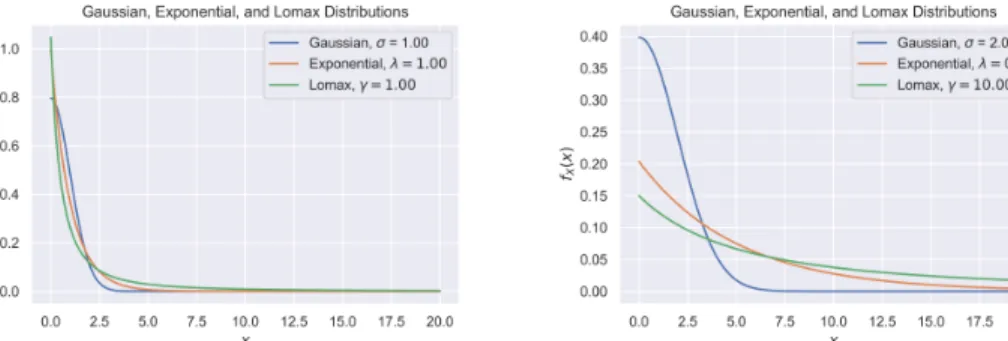
When considering different kinds of data, we are often interested in how they are distributed. Further, it is often important for us to characterize the tail of the dis-tribution. In some distributions, the frequencies of large elements drop very quickly (“light-tailed”), while in others, the frequencies of large elements drop more slolwy (“heavy-tailed”), meaning more samples are needed to see important elements. In this thesis, we give an algorithm that allows us to determine whether a distribution is “heavy-tailed” or “light-tailed”. For example, in Figure 1-1, we show the probability density functions of canonical heavy-tailed (Lomax), medium-tailed (exponential), and light-tailed (Gaussian) distributions, noting that the functional forms are some-what flatter in the end of the distribution for the heavy-tailed distribution and decays rather quickly for the light-tailed one.

Over the course of the thesis, we motivate the problem by mentioning several settings in which this attribute of distributions is important to consider in Chapter 1. We define important terminology and notation in Chapter 2. Then, we present an overview of our main contribution in Chapter 3, and in Chapter 4, we delve into the details of the algorithm and prove correctness.

Here, we first discuss settings in which our problem has arisen. Then, we present work that has been done to solve this problem in a different model and under different assumptions than ours. Next, we motive our setting and recapitulate work in that setting. Finally, we present our contributions.

Figure 1-1: Plots of probability density functions of three distributions. Lomax are heavy-tailed, exponential are medium-tailed, and Gaussian are light-tailed. When the parameters are set to all be one, we can see that the Lomax has the high weight for the largest elements, while the Gaussian has the small weight for the largest elements. This is exaggerated in the second plot by changing the parameters to make evident what it means for the tail to have more weight.

1.1

Motivation

In this section, we describe the real-world motivation for our problem.

Wanting to computationally understand properties of objects led to the develop-ment of property testing algorithms. In the presence of intractable amounts of data, we wish to test for these properties in a sublinear number of queries to the input. Indeed, distributions are such objects. Consider a multi-class classification problem with millions of input samples. We might want to understand whether the distribu-tion of that input data is uniform. For such problems, testers requiring a tiny number of queries exist.

In some settings, we may want to know what proportion of elements occur infre-quently. That is, we may wish to understand the nature of the tail of the distribution, and in particular, whether the tail has heavy or light weight. For example, Hsu et al. showed that in the presence of a stream of data following a Zipfian (particular kind of heavy-tailed) distribution, their approach improves significantly upon previ-ous approaches [13]. They evaluate Zipfianness on the entire dataset, but determining linearity of a log − log plot.

In other machine learning settings, the shape of the distribution affects the kinds of methods chosen [18]. Indeed, for certain distributions of data, we can prove that

we need to memorize training data in order to have any hope of generalization [11]. Thus, characterizing the tails of the distribution of data is of great importance for machine learning practitioners and learning theorists alike.

Similarly, in real-world settings, the completion time of jobs have been found to have heavy-tailed distributions. In the past, much of the analysis had been done with exponential workloads, so Harchol-Balter has analyzed the effect of heavy-tailed distributions on system design [12]. As properties differ between the exponential and heavy-tailed workloads, it would be valuable to be able to quickly determine which workload distribution we have.

Thus, the desire to quickly evaluate whether a distribution is heavy-tailed or not motivates the need for an algorithm to efficiently compute whether or not a distribution is heavy-tailed. We present what is to our knowledge a novel algorithm to solve this problem. The test statistic that we propose is guaranteed to work asymptotically.

1.2

Heavy-tailed Testing in Asymptotic Statistics

In this section, we discuss a prior approach to testing whether a distribution is heavy-tailed. This method is guaranteed to work as we approach infinitely many samples.

Bryson has proposed a tester for tail weight [9] that tester performs a simple hypothesis test to distinguish between an exponential distribution (𝑓𝑋(𝑥) = 𝜆𝑒−𝜆𝑥,

null hypothesis) and a Lomax distribution (𝑓𝑋(𝑥) = 𝛼_𝜆[︀1 + 𝑥_𝜆

]︀−(𝛼+1)

, alternative hy-pothesis). Their tester relies on a statistic called the conditional mean exceedance (CME):

CME(𝑥) = E [𝑋 − 𝑥|𝑋 ≥ 𝑥] (1.1)

The aim of the CME is to measure where the remaining mass is centered past a certain point 𝑥 in the distribution. We can express this as an integral:

CME(𝑥) = _¯1 𝐹 (𝑥) ∞ ∫︁ 𝑥 ¯ 𝐹 (𝑡)𝑑𝑡, ¯𝐹 (𝑥) = ∞ ∫︁ 𝑠=𝑥 𝑓𝑋(𝑠)𝑑𝑠 (1.2)

If the CME is increasing with 𝑥, then the tails are heavy. The tester given in the paper uses the fact that if CME(𝑥) = 𝑎 + 𝑏𝑥∀𝑥, then 𝑥 is drawn from a Pareto distribution. In the limit where 𝑏 → 0, we achieve the exponential distribution. After a series of transformations, the test statistic calculated in this paper, as a function of the samples received 𝑥(𝑖) for 𝑖 ∈ {1...𝑛}:

𝑇′ = 𝑥𝑥¯ (𝑛) (𝑛 − 1)¯𝑥2

𝐺𝐴

This statistic and method work well when we can get infinitely many samples from the distribution. Our result works in a similar setting albeit using a different charac-terization of what it means to be “heavy-tailed.”

1.3

Distribution Testing in Computational Statistics

In this section, we define the goals and setting of distribution testing as a computa-tional problem.

Distribution testing in the sublinear regime for discrete distribution usually takes the form of testing whether samples come from one of a certain class of distributions or are 𝜖-far from the closest distribution in that class, “far” being measured in a distance metric such as total variation.

The problem of distinguishing between classes of distributions with finitely many samples was first considered from a computational lens in [4] and later in [6]. The focus of the question became: how many samples do we require from a given distribution to distinguish it from something else? Since then, testers have been given for several properties of distributions [1] and under several conditions [3] [2].

As mentioned previously, the question of testing heavy-tailedness of a distribution has been studied in statistics [9]. To study it in the computational setting, we use several tools and results. We are concerned about how well quantiles calculated from samples concentrate, which is studied in [15] and [8].

1.4

Contributions

In this work, our main contribution is an algorithm that tests whether a distribution is heavy-tailed (as Lomax) or not (as exponential) a distribution is from a set of samples. The algorithm makes use of a test statistic we have developed that recovers the hazard rate characterization of heavy-tailedness. Our algorithm and test statistic make use of a new bucketing scheme based on dividing the support of a distribution into intervals with equal probability mass in each bucket defined by an interval. The test statistic we propose for heavy-tailedness is independent of the parameter of the distribution. In the rest of this section, we discuss these parts in more detail.

Our bucketing scheme (presented in section 4.1) is devised to capture the shape of the distribution even in parts of the distribution where we might not see many samples. This is especially valuable for heavy-tailed testing, since in light-tailed distributions, we expect to not see very many samples from the tail.

We present a test statistic (in Algorithm 1) for a general class of distributions that accurately captures the decreasing hazard rate condition for heavy-tailedness based on the aforementioned bucketing scheme. Importantly, this test statistic does not depend on the parameters of the underlying distribution, only the functional form. Further, this test statistic does not rely on seeing the end of the tail, meaning we can understand the tail behavior of a distribution from the beginning and middle of it.

We also present an efficient algorithm to calculate this tester from a set of samples. Our algorithm is presented in algorithm 1.

Chapter 2

Preliminaries

In this section, we present several preliminaries that prove useful throughout the thesis. In considering distributions and their properties, we make use of several statistics on the distributions and define them here. We present various definitions of “heavy-tailed”ness based on those statistics and then show how they relate. Then, we specify our setting and assumptions we make. Finally, we define distributions we reference that follow our assumptions.

2.1

Defining Heavy-Tailed Based on Statistics on

Dis-tributions

In this section, we provide two definitions for the notion of “heavy-tailed” and show how they relate. We say that a distribution has Probability Density Function (PDF) 𝑓𝑋(𝑥) and Cumulative Density Function (CDF) 𝐹𝑋(𝑥).

2.1.1

Conditional Mean Exceedance

The conditional mean exceedance (CME) is defined in [9] to be:

In the continuous setting, we can expand this in terms of the PDF 𝑓𝑋(𝑥) and the CDF 𝐹𝑋(𝑥) as: 𝐶𝑀 𝐸(𝑥) = ∞ ∫︀ 𝑥 (𝑠 − 𝑥)𝑓𝑋(𝑠)𝑑𝑠 1 − 𝐹𝑋(𝑥) (2.2) According to [9], a distribution is considered heavy-tailed if the CME is increasing for all 𝑥. The CME essentially captures the shape of tail by considering how the expectation of the tail of the distribution evolves throughout the tail. Thus, if it is increasing, the further into the distribution we go, the more that remains.

This definition considers an exponential distribution the canonical “medium-tailed” distribution and the Lomax distribution the canonical “heavy-tailed” distribution. In practical settings, this metric is valuable, as it represents “decreasing failure rate” [12]: the longer a job has been alive (as 𝑥 increases), the longer it is expected to stay alive (E(𝑋 − 𝑥|𝑋 ≥ 𝑥) increasing).

2.1.2

Hazard Rate

The hazard rate (HR) is defined in [17] to be:

𝐻𝑅(𝑥) = 𝑓𝑋(𝑥) 1 − 𝐹𝑋(𝑥)

(2.3)

A distribution with hazard rate that is a decreasing function of 𝑥 is considered to be heavy-tailed [14]. The hazard rate definition captures the fact that the significance of a given point relative to the tail decreases as we go further into the distribution.

2.1.3

Relating CME and HR definitions

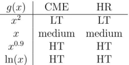
In this section, we consider the relationship between the two definitions of “heavy-tailed” presented in the previous section. Both characterizations (1) and (2) both treat the exponential distribution as “medium-tailed.” Indeed, calculation of the CME and HR of various distributions of the form 𝑒−𝑔(𝑥) shows that they agree in many cases (Table 2.1).

𝑔(𝑥) CME HR

𝑥2 _{LT LT}

𝑥 medium medium

𝑥0.9 _{HT HT}

ln(𝑥) HT HT

Table 2.1: How 𝑒−𝑔(𝑥) is classified by CME and HR. HT is heavy-tailed and LT light-tailed.

According to [17], the CME is the reciprocal of the hazard rate function of the equilibrium distribution of the CDF 𝐹𝑋(𝑥), which essentially “accumulates” the weight

in the tail.

Thus, there is a relationship between the two; we choose to use the HR defini-tion, since we are able to immediately relate it to a bucketing scheme we propose in Section 4.1.

2.2

Setting and Assumptions

Continuous Distribution

We consider continuous distributions on [0, ∞). We say that a distribution has Proba-bility Density Function (PDF) 𝑓𝑋(𝑥) and Cumulative Density Function (CDF) 𝐹𝑋(𝑥).

Monotone Decreasing

We assume that the PDF 𝑓𝑋 of the distribution is monotone decreasing. That is,

𝑓𝑋(𝑥1) ≥ 𝑓𝑋(𝑥2) when 𝑥1 < 𝑥2. In a real-world setting, this assumes that we know

how to sort elements by their frequency. While this is a somewhat strong assumption to make in some settings, in others, it is reasonable. For example, when considering job lengths, we often can make this assumption, at least in the tail.

Lipschitz Inverse CDF

We assume that the inverse CDF of a distribution is Lipschitz on [0, 𝑐2], where 𝑐2 < 1

interested in, this is a reasonable assumption.

Query Model

We have sample access to the distribution. When we query the distribution, we are returned one iid sample from the distribution. Thus, the sample complexity is exactly the query complexity.

2.3

Notation

We say that a distribution has Probability Density Function (PDF) 𝑓𝑋(𝑥) and

Cumu-lative Density Function (CDF) 𝐹𝑋(𝑥). A set of 𝑛 samples drawn from a distribution

with PDF 𝑓𝑋 is denoted 𝑋1, 𝑋2, ..., 𝑋𝑛. The order statistic at index 𝑛𝑖 of this set of

samples is denoted 𝑋(𝑛𝑖). The mean of the 𝑋(𝑛𝑖) is denoted 𝜇𝑖 and the variance 𝜎

2 𝑖.

The endpoints and lengths of equal weight buckets during the continuous interpreta-tion are denoted as I(𝑥), L(𝑥). Upon discretizainterpreta-tion, we switch to the use of 𝐼[𝑖], 𝐿[𝑖]. The number of samples is denoted by 𝑛, the number of buckets by 𝑘, and the index of the considered bucket by 𝑖.

2.4

PDF, CDF of Continuous Distributions

Based on these assumptions and setting, we use the names of well-known distributions in slightly different ways to common use. Thus, in this section we define the various distributions that are referenced throughout the paper as are relevant in our setting.

Exponential

The cutoff between heavy-tailed and light-tailed distributions according to both the CME and HR definitions is the exponential distribution. The continuous exponential distribution requires parameter 𝜆 > 0 has probability density function (PDF):

and cumulative density function (CDF):

𝐹𝑋(𝑥) = 1 − 𝑒−𝜆𝑥 (2.5)

The quantile function is:

𝐹_𝑋−1(𝑥) = −1

𝜆 ln 1 − 𝑥 (2.6)

Lomax

The Lomax distribution requires parameters 𝛼 > 0, 𝜆 > 0 and has PDF:

𝑓𝑋(𝑥) = 𝛼 𝜆 [︁ 1 + 𝑥 𝜆 ]︁−(𝛼+1) (2.7) and CDF: 𝐹𝑋(𝑥) = 1 − [︁ 1 + 𝑥 𝜆 ]︁−𝛼 (2.8) The quantile function is:

𝐹_𝑋,𝐿−1(𝑥) = 𝜆 (︂ 1 (1 − 𝑥)1/𝛼 − 1 )︂ (2.9)

We consider this the canonical “heavy-tailed” distribution.

Half-Gaussian

The half-Gaussian distribution requires parameter 𝜎 and has PDF:

𝑓𝑋(𝑥) = 2 𝜎√2𝜋𝑒 −1₂₍𝑥_𝜎)2 ; 𝑥 ∈ [0, ∞) (2.10) and CDF: 𝐹𝑋(𝑥) = erf (︂ 𝑥 𝜎√2 )︂ (2.11) The quantile function is:

Chapter 3

Overview of Main Result

In this section, we present our main result (Theorem 4.4.1) and discuss an overview of its proof. We specify the steps required to prove the result and expand upon them in Chapter 4. Further, we briefly explain extensions we believe we can make to our result.

3.1

Result

Theorem 3.1.1. There exists an algorithm that distinguishes between Lomax distri-butions with 𝛼 = 1 and exponential distridistri-butions. This algorithm is guaranteed to succeed as the number of samples gets large with a sufficient number of buckets. Such an algorithm is given in Algorithm 1.

Our algorithm solves the problem solved in [9] in a new way. While they develop a test statistic to distinguish between Lomax distributions and exponential distributions based on the CME characterization (Section 2.1.1), our test statistic distinguishes between Lomax distributions and exponential distributions by means of the hazard rate characterization of heavy-tailedness.

To develop such an algorithm, we make use of an equal weight bucketing scheme (Section 4.1). We develop a test statistic using this bucketing scheme that is equiva-lent to the hazard rate condition for heavy-tailedness and consider its concentration

to consider the sample complexity and success probability of the algorithm. For this, we use the asymptotic normality of the order statistic.

In order to show that the test statistic succeeds asymptotically, we use the fact that each of the random variables in the test statistic concentrate well. The random variables are order statistics (discussed in Section 4.3.3) and we use results from the literature [15] showing their concentration in Section 4.4.2. We then evaluate a prob-abilistic lower bound for the distance in our statistic between the Lomax distribution and the threshold (equivalent to the statistic for the exponential distribution). From this bound, we show that with enough samples, we can concentrate well enough. The probability with which this gap is significant would represent the success probability of the test.

3.2

A Note

We expect that this result can be extended in to a finite sample scenario. We can make use of the fact that we can characterize the distribution of the order statistics of a uniform random variable on [0, 1] well. We can then show using the delta method [16] that the standard deviation of an order statistic from a uniform distribution can be transformed into a standard deviation for an arbitrary distribution, allowing us to extend results about the former to arbitrary distributions. (This calculation for the transformed standard deviation is analogous to the result from [15] for the standard deviation of the order statistics of an arbitrary distribution.) By bounding the probability of failure, we can give a parameterized sample complexity.

Likewise, we expect that this result can be extended to distinguish broader classes of distributions, for example, light-tailed from Lomax. Our exact test statistic (given in Theorem 4.3.1) certainly works to distinguish general light-tailed and heavy-tailed distributions, so in order to make this extension, we would require that approxima-tions we make hold in the more general case.

Chapter 4

Algorithm

In this section, we expand upon our main result, that there exists an algorithm re-quiring to test whether a distribution is a Lomax with 𝛼 = 1 (hereafter referred to as Lomax) or exponential, and such an algorithm (Theorem 4.4.1). First, we discuss an equal weight bucketing scheme in Section 4.1. Then, we present the algorithm to test heavy-tailedness that makes use of that scheme (Section 4.2). Next, in Section 4.3, we show that the test statistic used in the algorithm correctly reflects the property we are testing. Finally, we consider sample complexity. To do this, we utilize re-sults regarding the order statistic and its concentration, then show that with enough samples, the test statistic for the Lomax distribution will be far away from the test statistic for the exponential (Section 4.4.2, Section 4.4.3).

4.1

Equal Weight Buckets

In this section, we motivate and define Equal Weight Buckets.

Dividing the support of a distribution into buckets is a well-known approach in distribution testing and is used in [7], [5], [10]. In essence, by considering the distri-bution on these buckets, we often can see trends that are less susceptible to sampling noise. In this case, the weight in the tail of a distribution is intrinsically linked to how quickly the distribution decays, which is reflected by the changing lengths of the buckets. Further, in typical bucketing schemes, the support is divided in the same

way regardless of the nature of the distribution, which in this setting would lead to very few samples being seen in buckets falling in the tail of the distribution. For these reasons, we can instead bucket the distribution into buckets containing equal weight. That way, we expect each bucket to have an equal number of samples fall in it. The lengths of these buckets, however, will vary. These equal weight buckets are equivalent to considering the quantiles of the distribution.

In this section, we refer to PDF of the distribution we are trying to test as 𝑓𝑋 and

the corresponding CDF as 𝐹𝑋. The endpoints of the buckets are given by I(·) and

their lengths by L(·). The “weight” refers to probability mass. First, we derive and define the notion of equal weight buckets according to the PDF and CDF and then explain how they are generated from samples.

The endpoints of the buckets are determined by the inverse of the CDF, giving us that in general: I(𝑥) = 𝐹𝑋−1(𝑥) (4.1) I(𝑖; 𝑘) = 𝐹𝑋−1 (︂ 𝑖 𝑘 )︂ ∀𝑖 ∈ {1, 2, ..., 𝑘 − 1} (4.2)

where 𝑖 is the index of the interval, and there are 𝑘 intervals1. For now, we derive the expressions for the continuous notion of these buckets: if we wanted to find the point in the support at which 𝑥 of the weight has been achieved, and the rate at which the weight changes, we can use the continuous versions. In Section 4.3.2, we describe how we discretize this. The derivative 𝑑𝐼_𝑑𝑖 gives us the length of the intervals. By chain rule: 𝑑 𝑑𝑥𝑓 −1 (𝑥) = 1 𝑓′_(𝑓−1_(𝑥))

Here, we have that:

𝐹𝑋(𝑥) = 𝑥 ∫︁ 0 𝑓𝑋(𝑥′)𝑑𝑥′ ⇐⇒ 𝑓𝑋(𝑥) = 𝑑 𝑑𝑥𝐹𝑋(𝑥)

1_{𝑖 = 𝑘 is not included since these distributions have infinite support and therefore lim} 𝑥→1𝐹

−1 𝑋 (𝑥) =

Thus, the lengths of the intervals are: L(𝑥) = 𝑑 𝑑𝑥𝐹 −1 𝑋 (𝑥) = 1 𝐹_𝑋′ (𝐹_𝑋−1(𝑥)) = 1 𝑓𝑋(𝐹𝑋−1(𝑥)) (4.3)

The rate of change of the lengths of the intervals are: 𝑑 𝑑𝑥L(𝑥) = −1 𝑓𝑋(𝐹𝑋−1(𝑥))2 · 𝑓_𝑋′ (𝐹_𝑋−1(𝑥)) · 1 𝑓𝑋(𝐹𝑋−1(𝑥)) (4.4)

4.2

Statement of the Algorithm

In this section, we present the algorithm and explain how it works. At a high level, the algorithm calculates a test statistic whose correctness we show in Section 4.3. In order to do this, we draw 𝑛 samples (determining 𝑛 is discussed in Section 4.4.3) and split them into buckets as described in Section 4.3.2. We present the algorithm in Algorithm 1.

Algorithm 1 Heavy-Tailed (Lomax) Test

1: 𝒮 ← 𝑛 samples from the distribution 2: Split 𝒮 randomly into disjoint 𝒮1, 𝒮2, 𝒮3

3: Sort 𝒮1, 𝒮2, 𝒮3

4: Split into 𝑘 equal weight buckets and determine interval endpoints I

5: Calculate L[i] = I[i + 1] - I[i] and dL[i] = L[i+1] - L[i]

6: Calculate S[i] = _{𝑑𝐿[𝑖]}𝐿[𝑖] for 𝑖 ∈ {1, 2, ..., 𝑘 − 2}

7: if 𝑆[𝑖] < 1 − _𝑘𝑖 −1

2 gap for 𝑖 ∈ {𝑐1· 𝑘, ..., 𝑐2· 𝑘} then

8: PASS

9: else

10: FAIL

The algorithm breaks the set of samples first into three sets as described in Sec-tion 4.3.3 and each of them into 𝑘 equal weight buckets by determining the end points of the buckets to be every 𝑛/𝑘𝑡ℎ sample. The way 𝑘 is set is discussed in Section 4.4.4. Indeed, in Section 4.3.3, we discuss how this allows us to analyze the statistic in terms of the order statistics. Subsequently, the algorithm calculates the lengths and the change in lengths of the buckets and computes a test statistic 𝑆 for 𝑖 ∈ {𝑐1 · 𝑘, ..., 𝑐2 · 𝑘}, where 0 < 𝑐1 < 𝑐2 < 1. We discuss the correctness of this test

statistic in Section 4.3 and justify the range of 𝑖 considered in Section 4.4.3. The threshold considered is the threshold given by the derivation of the statistic with some adjustment for the class of distributions we seek to distinguish between. The specifics of the gap mentioned are discussed in Section 4.4.3.

4.3

Test Statistic

In this section, we present a test statistic based on the idea of equal weight buckets that verifies the hazard rate condition on the tail. First we derive the tester from the hazard rate definition given in Section 2.1.2. Then, we show that we can use an approximation to the derivative to we can calculate the test statistic from samples. Finally, we motivate the use of order statistics and state the test statistic in terms of order statistics.

4.3.1

Derivation of Tester

The hazard rate condition for being heavy-tailed can be rearranged to give a con-dition on the tail of a distribution. Viewing this tail concon-dition from the lens of the aforementioned equal weight buckets, we get the following theorem.

Theorem 4.3.1. If for all 𝑖:

L(𝑥)|𝑥=𝑖/𝑘 𝑑

𝑑𝑥L(𝑥)|𝑥=𝑖/𝑘

< 1 − 𝑖 𝑘

then the underlying distribution is heavy-tailed according to the hazard rate definition.

Proof. According to [14], if the hazard rate of a distribution is decreasing, then the distribution is heavy-tailed. Let 𝑓𝑋(𝑥) be the PDF of a distribution and 𝐹𝑋(𝑥) the

implies: 𝑑 𝑑𝑥 𝑓𝑋(𝑥) 1 − 𝐹𝑋(𝑥) = (1 − 𝐹𝑋(𝑥))𝑓 ′ 𝑋(𝑥) − 𝑓𝑋(𝑥)(−𝑓𝑋(𝑥)) (1 − 𝐹𝑋(𝑥))2 < 0 (4.5) ⇒ (1 − 𝐹𝑋(𝑥))𝑓𝑋′ (𝑥) − 𝑓𝑋(𝑥)(−𝑓𝑋(𝑥)) < 0 (4.6) ⇒ −𝑓𝑋(𝑥) 2 𝑓_𝑋′ (𝑥) < 1 − 𝐹𝑋(𝑥) ⃒ ⃒ ⃒ ⃒ 𝑥=𝐹_𝑋−1(𝑖 𝑘) (4.7) ⇒ −𝑓𝑋(𝐹 −1 𝑋 ( 𝑖 𝑘)) 2 𝑓′ 𝑋(𝐹 −1 𝑋 ( 𝑖 𝑘)) < 1 − 𝐹𝑋 (︂ 𝐹_𝑋−1(︂ 𝑖 𝑘 )︂)︂ = 1 − 𝑖 𝑘 (4.8)

Equation (4.7) involves a sign change since we assumed that 𝑓𝑋(𝑥) is monotone

decreasing, and so its derivative must be negative. This derivation gives us a condition on the tail of the distribution which, if satisfied, implies that the distribution is heavy-tailed. From Equation (4.3) and Equation (4.4) in the previous section, we find that we can satisfy this condition when considering the ratio of the length of the buckets to the rate of change of the derivatives:

𝐿(𝑥) 𝑑 𝑑𝑥𝐿(𝑥) = 𝐿(𝑥) −𝑓′ 𝑋(𝐹 −1 𝑋 (𝑥))𝑓𝑋(𝐹𝑋−1(𝑥))−2𝐿(𝑥) = −𝑓𝑋(𝐹 −1 𝑋 (𝑥))2 𝑓′ 𝑋(𝐹 −1 𝑋 (𝑥)) ⃒ ⃒ ⃒ ⃒ 𝑥=_𝑘𝑖 = −𝑓𝑋(𝐹 −1 𝑋 ( 𝑖 𝑘)) 2 𝑓′ 𝑋(𝐹 −1 𝑋 (𝑘𝑖)) (4.9)

Thus, if this ratio is less than 1 −_𝑘𝑖∀𝑖, then the distribution is heavy-tailed. Likewise, if the ratio is greater than 1 − _𝑘𝑖∀𝑖, then the distribution is light-tailed.

In this work, we show that this threshold adjusted by a gap works to distin-guish between the Lomax and exponential distributions, but Theorem 4.3.1 holds for general heavy-tailed and light-tailed distributions. Indeed, we could use the latter statement, that the ratio being greater than 1 −_𝑘𝑖 implies light-tailedness as justifica-tion for the use of 1 −_𝑘𝑖 as the threshold between Lomax distributions and light-tailed distributions.

This theorem also leads us to the following corollary for distributions of the form 𝑓𝑋(𝑥) = 𝐶𝑒−𝜆𝑔(𝑥).

𝐶, 𝜆 are constants, if 𝐻𝑅𝑓(𝑥) > 𝑔′(𝑥), then 𝑓𝑋(𝑥) is heavy-tailed, and if 𝐻𝑅𝑓(𝑥) <

𝑔′(𝑥), then it is light-tailed. If 𝐻𝑅𝑓(𝑥) = 𝑔′(𝑥), then 𝑓𝑋(𝑥) is the exponential

distri-bution.

4.3.2

Tester in Terms of Buckets

Since we are drawing samples from a distribution and do not learn the distribution, we must approximate this statistic from the drawn samples. We can do this by approximating the derivative by the difference quotient. For the kinds of distributions we consider, we can make this approximation without incurring too much error due to the Lipschitz-ness of the PDF.

Lemma 4.3.2. When the derivative of a function 𝑔 is 𝐵 − 𝐿𝑖𝑝𝑠𝑐ℎ𝑖𝑡𝑧 for 𝐵 = 𝜖/∆𝑥, and the derivative 𝑔′(𝑥) is monotone, then approximating 𝑔′(𝑥) by the difference quo-tient 𝑔(𝑥+Δ𝑥)−𝑔(𝑥)_Δ𝑥 incurs no more than 𝜖 additive error.

Proof. By intermediate value theorem, there exists some point 𝑥′ ∈ [𝑥, 𝑥 + ∆𝑥], s.t.,

𝑔′(𝑥′) = 𝑔(𝑥 + ∆𝑥) − 𝑔(𝑥) ∆𝑥

|𝑔′(𝑥′) − 𝑔′(𝑥)| ≤ |𝑔′(𝑥 + ∆𝑥) − 𝑔′(𝑥)| ≤ 𝐵 · ∆𝑥 = 𝜖 (4.10)

Applying this to the inverse CDF, if 𝑓𝑋(𝑥) is 𝐵1−Lipschitz and 𝑓𝑋′ (𝑥) is

mono-tone, then approximating the derivative of the 𝐹_𝑋−1(𝑥) by the difference quotient

𝐹_𝑋−1((𝑖+1)/𝑘)−𝐹_𝑋−1((𝑖)/𝑘)

1/𝑘 incurs no more than

𝐵1

𝑘 additive error. Thus, for large enough

𝑘, we can make the difference quotient approximation and derive a statistic in terms of the samples from the distribution. We derive the exact bounds in Section 4.4.4.

equivalent is as follows: 𝑔(𝑥)|_𝑥=𝑖 𝑘 = 𝑔[𝑖] (4.11) 𝑑 𝑑𝑥𝑔(𝑥) ≈ 𝑔(𝑥 + ∆𝑥) − 𝑔(𝑥) ∆𝑥 ⃒ ⃒ ⃒ ⃒ 𝑥=_𝑘𝑖,Δ𝑥=1_𝑘 = 𝑔( 𝑖+1 𝑘 ) − 𝑔( 𝑖 𝑘) 1/𝑘 (4.12) = 𝑘 (︂ 𝑔(︂ 𝑖 + 1 𝑘 )︂ − 𝑔(︂ 𝑖 𝑘 )︂)︂ = 𝑘 (𝑔[𝑖 + 1] − 𝑔[𝑖]) (4.13)

Using this to expand the test statistic, and approximating the derivative for both 𝐿(𝑥) = _𝑑𝑥𝑑𝐼(𝑥) and _𝑑𝑥𝑑𝐿(𝑥) = _𝑑𝑥𝑑22𝐼(𝑥), we get: 𝑆[𝑖] = _(︁ (𝐼[𝑖 + 1] − 𝐼[𝑖])/(1/𝑘) 𝐼[𝑖+2]−𝐼[𝑖+1] 1/𝑘 − 𝐼[𝑖+1]−𝐼[𝑖] 1/𝑘 )︁ /(1/𝑘2₎ = (𝐼[𝑖 + 1] − 𝐼[𝑖]) 𝑘(𝐼[𝑖 + 2] − 2𝐼[𝑖 + 1] + 𝐼[𝑖]) (4.14)

4.3.3

Tester in Terms of Order Statistic

In order to calculate the endpoints of the equal weight buckets, we draw a set of samples, sort them, and then consider the samples at indices _𝑘𝑖 · 𝑛; 𝑖 ∈ {0, 1, ...𝑘}. These samples are known as the order statistics at those indices. The concentration of order statistics has long been studied [8], [15]; results from this literature are used and cited.

We randomly divide the set of samples 𝒮 drawn from the distribution into three subsets 𝒮1, 𝒮2, 𝒮3 ⊂ 𝒮 such that 𝒮1∪ 𝒮2∪ 𝒮3 = 𝒮, 𝒮1∩ 𝒮2∩ 𝒮3 = ∅, and |𝒮1| = |𝒮2| =

|𝒮3|. Then, we calculate 𝑋(_𝑘𝑖·𝑛) from 𝒮1, 𝑋(𝑖+1_𝑘 ·𝑛)from 𝒮2, and 𝑋(𝑖+2_𝑘 ·𝑛) from 𝒮3. Thus,

the three order statistics considered for each test statistic are independent, as they are calculated from different sets of samples, which makes the analysis easier. In terms of the order statistic, and approximating the derivative as the difference divided by the length, we get that the aforementioned tester can be written as follows in terms of the order statistic:

𝑆 = (︁ 𝑋₍𝑖+1 𝑘 ·𝑛)− 𝑋( 𝑖 𝑘·𝑛) )︁ 𝑘(︁𝑋₍𝑖+2 𝑘 ·𝑛)− 2 · 𝑋( 𝑖+1 𝑘 ·𝑛)+ 𝑋( 𝑖 𝑘·𝑛) )︁ < 1 − 𝑖 𝑘∀𝑖 ⇒ heavy tailed (4.15)

Defining 𝜆𝑖 = _𝑘𝑖, we can write this as:

𝑆 = (︀𝑋(𝜆𝑖+1·𝑛)− 𝑋(𝜆𝑖·𝑛) )︀

𝑘(︀𝑋(𝜆𝑖+2·𝑛)− 2 · 𝑋(𝜆𝑖+1·𝑛)+ 𝑋(𝜆𝑖·𝑛)

)︀ < 1 − 𝜆𝑖∀𝑖 ⇒ heavy tailed (4.16)

4.4

Sample Complexity and Concentration

In this section, we present the main theorem of this work, an algorithm distinguishes between exponential and Lomax with 𝛼 = 1. We analyze the value of the test statistic for a Lomax distribution when the order statistics concentrate well and show that if enough samples are drawn and enough buckets used, we expect that the test statistic for a Lomax distribution should be far from that for the exponential. Likewise, with enough samples and buckets, the test statistic for an exponential be close to the true value. We cite an old result showing that the order statistic is asymptotically normally distributed and use that to show that with enough samples, the test statistic will lie in the expected region. Finally, we computationally verify that the gap is significant with enough samples.

4.4.1

Statement of Main Result and Proof Outline

We restate the main theorem of our work.

Theorem 4.4.1. There exists an algorithm that distinguishes between Lomax distri-butions with 𝛼 = 1 and exponential distridistri-butions. This algorithm is guaranteed to succeed as the number of samples gets large with a sufficient number of buckets. Such an algorithm is given in Algorithm 1.

In the rest of this section, we show first how the order statistic concentrates. Next, we show that when an adequate number of samples have been drawn, there is a gap between the statistic evaluated for the Lomax and the threshold. Then, we determine the number of buckets required in order to accurately make the difference quotient approximation to the derivative as discussed in lemma 4.3.2. We finally show a computational validation of our theoretical result.

4.4.2

Asymptotic Normality of Order Statistic

A natural question is how to characterize the distribution of an order statistic. Ac-cording to [15], order statistics from continuous distributions that do not vanish and away from the ends behave asymptotically like normal distributions. The second condition is formalized by stating that the ratio of the index 𝑛𝑖 of the order statistic

in question to 𝑛, the number of samples must be a constant 𝜆𝑖 away from 0 and 1.

Thus, we can use this asymptotic normal approximation when considering quantiles of the distribution, as we are, since in this case, 𝜆𝑖 = _𝑘𝑖 for 𝑖 ∈ 1, ..., 𝑘 − 1.

The proof proceeds by taking a Taylor expansion of the PDF and discarding high order terms. Thus, by quantifying the error incurred by discarding these higher order terms, we can understand how much error we incur by making this normal approximation.

According to Theorem 2 in this paper, the mean and variance of the order statistics are 𝜇𝑖 = 𝐹_𝑋−1(𝑥), 𝜎𝑖2 =

𝜆𝑖(1−𝜆𝑖)

𝑛𝑓𝑋(𝐹_𝑋−1(𝜆𝑖))

2. Further, with enough samples, this should converge in distribution to normal. We use this result without proving it here. To convert this to a with high probability bound, we can use the inverse transform of a uniform normal variable and apply the delta method to show high concentration of the order statistics of the uniform implies high concentration of the order statistics of an arbitrary distribution.

4.4.3

Distinguishing Between Exponential and Lomax WHP

In this section, we calculate the statistic for exponential and Lomax distributions and show that if the individual order statistics concentrate well, then the gap between the test statistics for exponential and Lomax is large and discernible.

Lemma 4.4.2. The gap between a Lomax distribution with parameter 𝛼 = 1 and an exponential distribution in our test statistic is 𝑂(1) with enough samples and 𝑖 = Θ(𝑘). Proof. We calculate the value of the test statistic for the Lomax distribution and for exponential when the values of the order statistics differ from their expectations by some parameter 𝜂 number of standard deviations. We then show that if we draw

enough samples, we still will have an appreciable gap between the Lomax distribution and the exponential in our statistic.

The upper and lower bounds when the realization of the 𝑖𝑡ℎ _{order statistic varies}

by 𝜂𝜎𝑖 from its mean 𝜇𝑖 are as follows:

E [𝑆] ≥ 1 𝑘 𝜇𝑖+1− 𝜂𝜎𝑖+1− (𝜇𝑖+ 𝜂𝜎𝑖) 𝜇𝑖+2+ 𝜂𝜎𝑖+2− 2(𝜇𝑖+1− 𝜂𝜎𝑖+1) + 𝜇𝑖+ 𝜂𝜎𝑖 (4.17) = 1 𝑘 𝜇𝑖+1− 𝜇𝑖− 𝜂(𝜎𝑖+1+ 𝜎𝑖) 𝜇𝑖+2− 2𝜇𝑖+1+ 𝜇𝑖+ 𝜂(𝜎𝑖+2+ 𝜎𝑖+1+ 𝜎𝑖) (4.18) E [𝑆] ≤ 1 𝑘 𝜇𝑖+1− 𝜂𝜎𝑖+1− (𝜇𝑖− 𝜂𝜎𝑖) 𝜇𝑖+2− 𝜂𝜎𝑖+2− 2(𝜇𝑖+1+ 𝜂𝜎𝑖+1) − 𝜇𝑖+ 𝜂𝜎𝑖 (4.19) = 1 𝑘 𝜇𝑖+1− 𝜇𝑖+ 𝜂(𝜎𝑖+1+ 𝜎𝑖) 𝜇𝑖+2− 2𝜇𝑖+1+ 𝜇𝑖− 𝜂(𝜎𝑖+2+ 𝜎𝑖+1+ 𝜎𝑖) (4.20)

Note that these hold with high probability if we wish to bound 𝜂 or if 𝑛 is very large. Based on the discussion in Section 4.4.2, we have that the mean and standard deviation of the order statistic are defined as 𝜇𝑖 = 𝐹𝑋−1(𝜆𝑖) and 𝜎𝑖 =

𝜆𝑖(1−𝜆𝑖)

𝑛𝑓𝑋(𝐹𝑋−1(𝜆𝑖)) 2 where 𝜆𝑖 = _𝑘𝑖. Note that in general, with enough samples, even if 𝑓𝑋(𝐹𝑋−1(𝜆𝑖))2 is

very small, we can keep the variance small.

For the exponential distribution, just as in Equation (2.4) and Equation (2.5):

𝑓𝑋,𝐸(𝑥) = 𝛾𝑒−𝛾𝑥 (4.21)

𝐹𝑋,𝐸(𝑥) = 1 − 𝑒−𝛾𝑥 (4.22)

𝐹_𝑋,𝐸−1 (𝑥) = −1

𝛾 ln (1 − 𝑥) (4.23)

Likewise, setting 𝛼 = 1 and the other parameter to 𝛾 for the PDF defined in Equa-tion (2.7), we get that:

𝑓𝑋,𝐿(𝑥) = 1 𝛾(︁𝑥_𝛾 + 1)︁2 (4.24) 𝐹𝑋,𝐿(𝑥) = 1 − 1 𝑥 𝛾 + 1 (4.25) 𝐹_𝑋,𝐿−1 (𝑥) = 𝛾 (︂ 1 1 − 𝑥− 1 )︂ (4.26)

Denoting the distribution to which the parameter 𝛾 belongs by subscript, E for the exponential and L for the Lomax, we have:

𝜇𝐸,𝑖 = −1 𝛾𝐸 ln (1 − 𝜆𝑖) (4.27) 𝜎_𝐸,𝑖2 = 𝜆𝑖 𝑛𝛾2 𝐸(1 − 𝜆𝑖) = 𝑖 𝛾2 𝐸𝑛(𝑘 − 𝑖) (4.28) 𝜇𝐿,𝑖 = 𝛾𝐿 (︂ 1 1 − 𝜆𝑖 − 1 )︂ (4.29) 𝜎_𝐿,𝑖2 = 𝛾 2 𝐿𝜆𝑖 𝑛(1 − 𝜆𝑖)3 = 𝑘 2_𝑖𝛾2 𝐿 𝑛(𝑘 − 𝑖)3 (4.30)

Next, we calculate the upper bound for the test statistic calculated from samples from a Lomax distribution. We calculate such an upper bound when the realization of the 𝑖𝑡ℎ order statistic varies by 𝜂𝜎𝑖 from its mean 𝜇𝑖 (note that the 𝛾𝐿 have all factored

out and cancelled):

𝑆𝐿𝑖 = 1 𝑘 1 1−𝑖+1_𝑘 − 1 1−_𝑘𝑖 + 𝑘𝜂 (︁√︁ 𝑖+1 𝑛(𝑘−𝑖−1)3 + √︁ 𝑖 𝑛(𝑘−𝑖)3 )︁ 1 1−𝑖+2_𝑘 − 2 1 1−𝑖+1_𝑘 + 1 1−_𝑘𝑖 − 𝑘𝜂 (︁√︁ 𝑖+2 𝑛(𝑘−𝑖−2)3 + 2 √︁ 𝑖+1 𝑛(𝑘−𝑖−1)3 + √︁ 𝑖 𝑛(𝑘−𝑖)3 )︁ (4.31) ≤ 1 𝑘 1 𝑘−𝑖−1 − 1 𝑘−𝑖 + 2𝜂 (︁√︁ 𝑖+1 𝑛(𝑘−𝑖−1)3 )︁ 1 𝑘−𝑖−2 − 2 1 𝑘−𝑖−1 + 1 𝑘−𝑖 − 4𝜂 (︁√︁ 𝑖+2 𝑛(𝑘−𝑖−2)3 )︁ (4.32) = 1 𝑘 1 (𝑘−𝑖−1)(𝑘−𝑖) + 2𝜂 (︁√︁ 𝑖+1 𝑛(𝑘−𝑖−1)3 )︁ 2 (𝑘−𝑖−2)(𝑘−𝑖−1)(𝑘−𝑖) − 4𝜂 (︁√︁ 𝑖+2 𝑛(𝑘−𝑖−2)3 )︁ (4.33)

Similarly, we compute a lower bound for the statistic for the exponential. Here, too, all the 𝛾𝐸 factor out and cancel.

𝑆𝐸,𝑖= 1 𝑘 −1 𝜆𝐸 (︀ln(1 − 𝑖+1 𝑘 ) − ln(1 − 𝑖 𝑘))︀ − 𝜂 𝜆𝐸 (︁√︁ 𝑖+1 𝑛(𝑘−𝑖−1) + √︁ 𝑖 𝑛(𝑘−𝑖) )︁ −1 𝜆𝐸 (︀ln(1 − 𝑖+2 𝑘 ) − 2 ln(1 − 𝑖+1 𝑘 ) + ln(1 − 𝑖 𝑘))︀ + 𝜂 𝜆𝐸 √︁ 𝑖+2 𝑛(𝑘−𝑖−2) + 2 √︁ 𝑖+1 𝑛(𝑘−𝑖−1) + √︁ 𝑖 𝑛(𝑘−𝑖) )︁ (4.34) ≥ 1 𝑘 − ln(︀1 − 1 𝑘−𝑖)︀ − 2𝜂 √︁ 𝑖+1 𝑛(𝑘−𝑖−1) − ln(︁1 −_{(𝑘−𝑖−1)}1 2 )︁ + 4𝜂√︁_{𝑛(𝑘−𝑖−2)}𝑖+2 (4.35)

The distance between the exponential and the Lomax test statistic with arbitrarily small variances is:

𝑔 = |𝑆𝐸,𝑖− 𝑆𝐿,𝑖| = ⃒ ⃒ ⃒ ⃒ 𝑘 − 𝑖 − 2 𝑘 + 1 𝑘(𝑘 − 𝑖) − (︂ 𝑘 − 𝑖 − 2 2𝑘 )︂⃒ ⃒ ⃒ ⃒ (4.36) = 𝑘 − 𝑖 − 2 2𝑘 + 1 𝑘(𝑘 − 𝑖) = 1 2 − 𝑖 2𝑘 − 1 𝑘 + 1 𝑘(𝑘 − 𝑖) (4.37)

Note that we lower bounded the test statistic for the exponential using its Taylor expansion. From Theorem 4.3.1, we know that in the exact test statistic (𝑆*), we have that: 𝑆_𝐿* = 1 2− 𝑖 2𝑘 (4.38) 𝑆_𝐸* = 1 − 𝑖 𝑘 (4.39) gap* = 1 2− 𝑖 2𝑘 (4.40)

Thus, we almost exactly recover the gap in the exact statistic, reducing it by only

𝑘−𝑖−1

𝑘(𝑘−𝑖). In the next section, we describe what this implies about the required number

of buckets.

Note that we can actually reduce the value of the variances appreciably when 𝑛 is large enough without even strictly needing for 𝑛 → ∞. In particular, if 𝑛 = 𝑜(𝑘4_),

then the size of the standard deviation would be larger than the the combination of means causing terms to become negative. If 𝑛 = 𝑂(𝑘5_{), there are some 𝜂 for which}

this works and others for which it does not. If 𝑛 = Θ(𝑘6), then the term with the standard deviation becomes a factor of 1_𝑘 smaller than the rest (when 𝑖 = Θ(𝑘)). Thus, if 𝑛 = Ω(𝑘6), then there is a constant gap between the test statistics calculated for exponential and Lomax. In Section 4.4.5 , we show computationally that Lemma 4.4.2 holds for various parameter settings.

4.4.4

Number of Buckets Required

In this section, we calculate a lower bound on the number of buckets required for the approximation to the derivative to not cause conflation between a Lomax and an exponential distribution. Essentially, we want to find a 𝑘 such that the error incurred by the approximation to the derivative does not take up more than a quarter of the gap.

In particular, we would like for the gap after making the derivative approximation to still be half the gap in 𝑆*. From the calculation in Equation (4.36), the approxi-mation for the Lomax distribution increases the test statistic by an additive _𝑘1. Thus, we will require that for the exponential, we do not want to go below the exact value of the statistic by more than 1₄(︀1 − _𝑘𝑖 − 𝑘−𝑖

2𝑘 )︀, meaning that we want:

𝑘 − 𝑖 − 2 𝑘 + 1 𝑘(𝑘 − 𝑖) > 7 8 − 7𝑖 8𝑘 (4.41) 2 𝑘 < 1 8 − 𝑖 8𝑘 (4.42)

To satisfy this, we can use 𝑘 > _1−𝑐16

2. For the Lomax, the statistic with the approxi-mated derivative was in fact lower than the exact statistic, so it does not “encroach” on the gap.

4.4.5

Gap for Different Parameter Values

In this section, we present and discuss how the gap between the exponential and Lomax distribution varies with different settings of 𝑘, 𝑛, 𝜂.

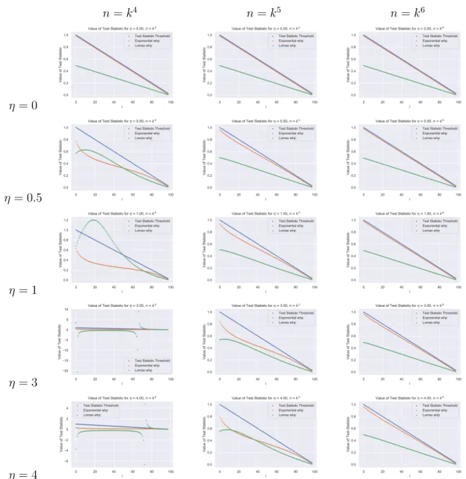
Figure 4-2 shows the gap for 𝑘 = 1000, Figure 4-1 shows the gap for 𝑘 = 100 for various values of 𝑛, 𝜂. In the rows of Figure 4-1 and Figure 4-2, we consider different values of 𝜂, the parameter that controls the number of standard deviations by which each order statistic differs from its expectation. As the order statistic is approximately normal, we need not consider more than 4 standard deviations away from the expectation. The rows show different values of 𝑛. We would expect that 𝜂 = 0 would represent the same gap as we would get if we did not consider the

𝑛 = 𝑘4 _{𝑛 = 𝑘}5 _{𝑛 = 𝑘}6 𝜂 = 0 𝜂 = 0.5 𝜂 = 1 𝜂 = 3 𝜂 = 4

deviations from expectation, and we expect that that should be independent of the number of samples, which is what we see in the first row.

In subsequent rows, we see some cases in which the gap is obvious and others in which there is no gap and perhaps even no clear meaning to the plot. When 𝜂 = 3, 4 and 𝑛 = 𝑘4, for certain values of 𝑖, either the value of the test statistic for Lomax has actually become negative.

Where Figure 4-2 shows the gap for 𝑘 = 1000, Figure 4-1 shows the gap for 𝑘 = 100. In comparing the plots, we can clearly see that the the smaller value for 𝑘 causes the statistic to “invade” the gap more due to a poorer approximation to the derivative.

𝑛 = 𝑘4 _{𝑛 = 𝑘}5 _{𝑛 = 𝑘}6 𝜂 = 0 𝜂 = 0.5 𝜂 = 1 𝜂 = 3 𝜂 = 4

Chapter 5

Conclusions and Next Steps

In this work, we presented a novel algorithm and test statistic for determining whether the tail of a continuous distribution is Lomax with 𝛼 = 1 or exponential. Our result differs from a result in [9] by using the hazard rate characterization of tail weight rather than CME as used by [9].

Our result relied on an equal weight bucketing scheme that we developed to cap-ture the shape of regions of the distribution where we may not see too many samples. We showed that using this bucketing scheme, we can exactly recover the hazard rate characterization, and when we calculate the buckets from samples, we incur little approximation error so long as we define a sufficient number of buckets.

We finally showed that if we draw enough samples, the distance between the test statistic for Lomax and the exponential is high and with enough buckets, any error incurred by approximating the derivative cannot interfere with how we classify the distribution.

We expect that this result can be extended to a finite sample setting by accurately determining the probability with which the order statistic is close to its expectation. This would allow us then to determine the number of samples required by fixing the number of standard deviations away from normal the order statistic falls with high probability. Further, our exact tester works for general heavy-tailed and light-tailed distributions, and we expect that our approximate tester can be extended to more general heavy- and light- tailed distributions.

Preliminary experiments also suggest this algorithm is practically useful. Future work will include evaluating the performance of the algorithm on synthetic and real-world data.

Bibliography

[1] Jayadev Acharya, Constantinos Daskalakis, and Gautam Kamath. Optimal test-ing for properties of distributions. In Proceedtest-ings of the 28th International Con-ference on Neural Information Processing Systems - Volume 2, NIPS’15, pages 3591–3599, Cambridge, MA, USA, 2015. MIT Press.

[2] Maryam Aliakbarpour, Ilias Diakonikolas, Daniel Kane, and Ronitt Rubinfeld. Private testing of distributions via sample permutations. In Advances in Neural Information Processing Systems 32, pages 10877–10888. Curran Associates, Inc. [3] Maryam Aliakbarpour, Ilias Diakonikolas, and Ronitt Rubinfeld. Differentially private identity and equivalence testing of discrete distributions. In International Conference on Machine Learning, pages 169–178.

[4] Tugkan Batu, Lance Fortnow, Ronitt Rubinfeld, Warren D. Smith, and Patrick White. Testing that distributions are close. pages 259–269.

[5] Tugkan Batu, Ravi Kumar, and Ronitt Rubinfeld. Sublinear algorithms for testing monotone and unimodal distributions. In Proceedings of the thirty-sixth annual ACM symposium on Theory of computing - STOC ’04, page 381. ACM Press.

[6] Tugkan Batu, Ravi Kumar, and Ronitt Rubinfeld. Sublinear algorithms for testing monotone and unimodal distributions. In Proceedings of the Thirty-sixth Annual ACM Symposium on Theory of Computing, STOC ’04, pages 381–390, New York, NY, USA, 2004. ACM.

[7] Lucien Birge. On the risk of histograms for estimating decreasing densities. 15(3):1013–1022. Publisher: Institute of Mathematical Statistics.

[8] Stephane Boucheron and Maud Thomas. Concentration inequalities for order statistics. 17(0).

[9] Maurice C. Bryson. Heavy-tailed distributions: Properties and tests. 16(1):61– 68.

[10] Clément L. Canonne, Themis Gouleakis, and Ronitt Rubinfeld. Sampling cor-rectors. 47(4):1373–1423.

[11] Vitaly Feldman. Does learning require memorization? a short tale about a long tail.

[12] Mor Harchol-Balter. The effect of heavy-tailed job size distributions on computer system design. page 17.

[13] Chen-Yu Hsu, Piotr Indyk, Dina Katabi, and Ali Vakilian. Learning-based fre-quency estimation algorithms.

[14] Dan Ma. The pareto distribution. https://statisticalmodeling.wordpress.com/2011/06/23/the-pareto-distribution/.

[15] Frederick Mosteller. On some useful "inefficient" statistics. 17(4):377–408. [16] Alex Papanicolaou. Taylor approximation and the delta method. page 6. [17] Chun Su and Qi-he Tang. Characterizations on heavy-tailed distributions by

means of hazard rate. 19(1):135–142.

[18] Yu-Xiong Wang, Deva Ramanan, and Martial Hebert. Learning to model the tail. In I. Guyon, U. V. Luxburg, S. Bengio, H. Wallach, R. Fergus, S. Vishwanathan, and R. Garnett, editors, Advances in Neural Information Processing Systems 30, pages 7029–7039. Curran Associates, Inc.