The analysis and synthesis of linear servomechanisms

THE ANALYSIS AND SYNTESIS OF LINEAR SERVOMECRANISMS

by

ALBERT CARRUTHERS HALL

. IT,

wE

10 1946

S.B., Agricultural and Mechanical College of Texas 1936

S.M., Massachusetts Institute of Technology 1938

SUBMITTED IN PARTIAL FULFILLbNT OF THE BEQUIREMENTS FOR THE DEGREE OF

DOCTOR OF SCIENCE

at the

MASSACHUSETTS INSTITUTE OF TECHNOLOGY 1943

Signature of Author

Signature Redacted

Department of Electrical Engineering, May 10, 1943 A

Signature Redacted

Signature Redacted

Chairman, Dept. Comm. on Gradu.atettudents

MITLibraries

DISCLAIMER NOTICE

Due to the condition of the original material, there are unavoidable

flaws in this reproduction. We have made every effort possible to

provide you with the best copy available.

Thank you.

The following pages were not included in the

original document submitted to the MIT Libraries.

This is the most complete copy available.

I

At

' 713

sq ii

COAPTER PAGE

ACKNOWIEDGMENTS

Advantages of a Closed-Cycle Control System 13

General Response Characteristics of Servomechanisms 22 II. MINIMUM INTEGRAL-SQUARED-ERROR

Servomechanism Response Criterion 33

Example: Type I Servo 37

Example: Third-Order Servomechanism 43 III. FUM&4iV4TAL PROPERTIES OF SERVOMECHANISM

TRANSFER-FUCTION LOCI 48

Graphical Calculation of the Error and Output

Functions 52

Nyquist's Stability Criterion 57

Transfer-Locus of Zero-Displacement-Error Servo 62 Transfer-Locus of Zero-elocity-Error Servo 66 Zero Acceleration-Error Servomechanisms 69 Shape of Transfer-Locus at Infinite Frequency 71

Ideal Zero-Displacement-Error Servo 73

IV. APPLICATION OF TRANSFER-LOCI TO THE ADJUSTMENT OF

SERVOMECHANISMS 76

Servomechanism Design Procedure 76

Factors Important in Servo Adjustment 77

CHAPTER _PAGE

Frequency Transformation ₈₀

Selection of the Gain Factor "K" 81

Example: Servomechanism with Third-Order

Transfor-Func tion 92

V.,

Zero Velocity-Error Systems 106

Minimum Velocity-Error Systems 131

Case I: h - 1; Under-Compensating

Integral-Controller 132

Case II: h>l; Over-Compensating

Integral-Controller 138

High-Gain Integral-Controller 144

Realization _{of Under-Compensating}

Integral-Control by Cascade Circuits 145

VI. THEORY OF PHASE-LEAD-CONTROLLERS ₁₅₀

Derivative Controller ₁₅₃

Basic Lead-Controller 162

Type I Servo with Basic Lead-Controller 167 Limitations Upon the Transfer-Functions of

Systems with Lead-Controllers 178.

Third-Order Transfer-Function Servomechanism with

Basic Lead-ontroller 186

Third-Order Transfer-Function Servo with CompounA

Third-Order Transfer-Junction Servo with Compound

Lead-Controller. Case 2: C3'1.0 204

Third-Order Transfer-Iunction Servo with Compound

Lead-Controller. Case 3: C3 1.0 208 Synthesis of Lead-Controllers: Generalization 214

VII. APPROXIMATION CRITZRIA ₂₁₉

VIII. THEORY OF MINIMUM VEOCITY-ERROR SERVOMEGHANISMS

PART 2 ₂₂₉

Systems Comprising both Integral- and

Lead-Controllers ₂₂₉

Example: Third-Order Transfer-Yunction Servo with

Basic Lead-Controller and Integral-Controller 235

Integral-Controller Design Limitations ₂₃₉

RLC Integral-Controller ₂₄₄

IX. BASIC CONTROLLER NETWORKS ₂₅₁

Under-Compensating Integral-Controller: Effect

of Source and Load Resistances 254

Under-Compensating Integral-Controller: Inductive

Circuit ₂₅₆

Basic Lead-Controller: _{Effect of Source and Load}

Resistances ₂₅₈

Basic Lead-Controller: Inductive Equivalent 261

Matching Lead-Controller 262

Matching Lead-Controller: Resistance of Voltage

CHAPTER PAGE Combined Basic Lead-Controller and

Integral-Controller: Case I, m =M 269

Combined Basic Lead-Controller and

Integral.-Controller: Case II, (X> 274

Combined Basic Lead-Controller and

Integral-Controller: Case III, ad 7 M 277

X. REGENERATIVE CONTROT-IES 281

Under-Compensating Integral-Controller 282

Basic Lead-Controller 284

Matching Lead-Controller 2S6

Combined Lead-Controller and Integral-Controller:

Attenuation Factors Equal 287

XI, CONSTANT-RESISTANCE CONTROLLERS 290

Under-Compensating Integral-Controller t

Constant-Resistance Network 300

Basic Lead-Controller: Constant-Resistance

Network 305

Combined Integral- and Basic-Lead Controller i

Constant-Resistance. Network 308

Matching Lead-Controller: Constant-Re si stance

Network 311

Bridged-T Equivalent of the Lattice 319

SUGGESTIONS FOR FURTHER WORK 323

The theory set forth in this thesis has been tested and proved

on numerous servo problems encountered by the Servomechanisms laboratory at M.I.T. In order to make the development inherently complete, a number of points have been discussed which have been

covered previously by other papers. Reference to these papers is made in the text; those of Black, 2, Nyquist,21 and Harris1 3

' are worthy of special reference and the paper by Bomberger and Weber,3 1 _,

which was not available to the author until most of the work was

completed, is particularly significant.

Chapter II, devoted to the minimum-integral squared error criterion, is included in the paper because of the frequency with which that criterion is applied in servo design. Those who are not specifically interested in that criterion can omit Chapter II without loss of continuity.

Acknowledgment is gratefully made to Professor G. S. Brown, the director of the Servomechanisms Laboratory in which much of

the work was done, for his interest and for the fact that it was he who was primarily responsible for arousing interest in servo design; to Professor H. L. Hazen for his continued interest and

encouragement; to Professor M. F. Gardner, Professor E. A. Guillemin, Professor J. C. Boyce, and Mr. H. T. Marcy for numerous helpful

suggestions; and especially to Mr. G. J. Schwartz for his careful reading of the paper and valuable criticisms.

Albert 0. Hall Cambridge, Massachusetts

ABSTRACT

This paper is a formulation of a servomechanism design proced-ure based primarily upon an analysis of the system response to

sinusoidal inputs of various frequencies. Although a knowledge of the transient performance of a servomechanism provides an excellent basis for predicting the response of the system to the conditions of a particular application, the complexity of most physical systems makes the computation of the transient perform-ance and the translation of the resulting information into physi-cal design criteria extremely laborious. On the other hand, knowledge of the response of the servomechanism to sinusoidal

inputs is not quite as useful in enabling a prediction to be made of the servo response to the conditions of most practical applications, but the computation of the sinusoidal response and the translation of this information into useful design criteria are much simpler.

The methods developed are based upon the characteristics of

the servomechanism transfer-function which is defined as the vec-tor ratio of the servo output to the difference between the

servo input _{and output for sinusoidal inputs of various}

fre-quencies. _{The characteristics of a servomechanism are completely} determined once its transfer-function is specified. Moreover,

physical devices that realize a prescribed transfer-function are readily synthesized if the given function is of such nature that such devices exist. This paper undertakes first to derive the

-2-interconnecting relations between particular servomechanism characteristics and the transfer-function of the servo, and sec-ond to synthesize devices that physically realize desired transfer-functions.

The study of transfer-function characteristics is aided by considering the transfer-function to be a vector and plotting the locus described by the tip of the vector as the frequency of the servo input is varied. The application of graphical analysis to this locus, termed a transfer-locus, facilitates the calcula-tion of certain servomechanism characteristics and provides a clearer insight to many servomechanism phenomena. It is also

shown how a knowledge of the transfer loci of a servomechanism enables the system to be so adjusted that optimum performance is

obtained.

The performance of a servomechanism may be unacceptable if either the steady-state error or the transient error is unsatis-factory under operating conditions. The steady-state error is

defined as the difference (or error) between the servomechanism output and its input under input conditions of such nature that this difference is either constant or varying periodically. The transient error is the difference between the servomechanism out-put and inout-put under inout-put conditions that result in a

non-periodic variation in that difference. This paper derives the form the servo transfer-function must possess if the steady-state error and the transient error are to fall below allowable limits. It is shown that, if necessary, certain compensating functions

Criteria are developed that serve as guides in the analysis,

application, and adjustment of the devices that physically real-ize the compensating functions.

Following the discussion of compensating functions, their

physical realization is considered and it is shown how several very different types of circuits may be synthesized that yield the desired function. Advantages and shortcomings of the various compensating devices are discussed.

TME _{ANALYSIS AND SYNT}aSIS OF LITEAR SERVOMECHANISMS}

INTRODUCTION

It is frequently necessary to control the position of a de-vice or the state of a process in accordance with indications or signals supplied by a suitable controlling instrument. If the power required to operate the device or process is large com-pared with the power available from the controlling instrument, means must be provided for effectively amplifying the controlling signals in order to secure proper operation of the device or proc-ess. The element that amplifies these signals and operates the device or process is known as an automatic controller, and the complete system, comprising the automatic controller, the con-trolling instrument that provides the automatic controller with signals, and the device or process being controlled, is known as

an automatic control system.

Automatic control systems, in general, comprise two types, namely, oPen-cycle control systems and closed-cycle control sys-tems. The signals supplied to the controller of an open-cycle control system are received solely from the controlling instru-ment instru-mentioned above, while in the case of the closed-cycle con-trol system additional signals that are proportional to the posi-tion of the device or the state of the process being controlled are received by the controller. Use of a closed-cycle control system permits much greater accuracy to be attained than is pos-sible with an open-cycle control system.

A closed-cycle control system is also termed a servomechanism.

Hazen1* _{has formally defined a servomechanism as "a}

power-amplify-ing _{device in which the amplifier element driving the output is}

actuated by the difference between the input to the servo and its output." _{Servomechanisms are used wherever accurate,} auto-matic control is desired. For example, they are employed to

steer ships, jr _{to control airplanesi'" to regulate temperature,'' 2} to maintain liquid levels, to control many military devices, and for general industrial process control.'1 6

'2 While a great deal

has been published describing particular types and applications of servomechanisms, relatively little has been written concern-ing the broader aspects of the problem of their analysis and design.

The type of servomechanism discussed in this paper is the type employed when results of highest accuracy are required, namely, the continuous-control type. This type of

servomechan-ism is distinguished by the fact that a definite and continuous

corrective action is developed by the servo-controller and ap-plied to the device being controlled no matter how small is the

error in the position of that device. This paper is devoted ex-clusively to the analysis of the continuous-control type of servomechanism.

If the performance of a system can be expressed

mathemati-cally by a linear differential equation with constant coefficients,

-6.-that system is said to be linear. While the following paper is

concerned with linear sevomechanisms only, the results are

guides to predicting the performance of systems with certain

non-linear characteristics. The load of many servomechanisms

in-cludes Coulomb friction, i.e., friction whose magnitude is

inde-pendent of velocity and whose direction is such as always to

oppose the direction of motion of the servo output. The effect

of a small force or torque of this type on an otherwise linear

system can be predicted approximately without the need of making

an exact analysis of the system, provided the analysis of the

otherwise linear system is known. The subsequent theory, however,

is devoted entirely to linear systems.

Most of the published works dealing with the subject of

automatic control have been concerned principally with the

de-scription of the performance and application of a particular

automa'tic control system. Certain earlier papers of analytic

nature are listed in the bibliography under

Further reference is made to these papers in subsequent portions

of this paper.

The theory of feedback amplifiers is applicable in many

respects to the analysis of servomechanisms and the similarity

between feedback amplifiers and servomechanisms is stressed at

appropriate points in the paper. Certain important basic

differ-ences, however, exist between the two devices. One is that a

accuracy; much design effort, therefore, is devoted to secur-ing as small a servo error as practicable. On the other hand, most feedback amplifier theory is relatively unconcerned with this problem. A second essential difference arises from the fact that the load on a servomechanism is generally such a com-paratively massive member that the important part of the

fre-quency response of the complete system lies in and below the low audio frequency band. On the other hand, most feedback am-plifier theory is concerned with securing good response at and above high audio frequencies. The frequency response of

servo-mechanisms can be extended and the servo response improved by em-ploying compensating circuits whose characteristics become unim-portant at frequencies higher than the audio range. In most

cases, therefore, the effects of parasitic inductances and

capaci-tances present in these compensating circuits are relatively un-important. On the other hand, the frequency response of most feedback amplifiers is limited by the parasitic inductances and capacitances of the amplifier circuit. The type of compensating circuits applicable in servomechanism controllers may not be em-ployed to extend the frequency range of amplifiers, therefore,

because of the effect of the parasitic elements on these circuits at high frequencies. References are made to feedback amplifier

theory and portions of the theory are utilized, but, in general, the results in this paper have been developed along separate

-8-Methods of Analysis

The design of electrical equipment of all types is aided by obtaining, by calculation or laboratory measurements, the response of the equipment to certain test conditions so chosen that the resulting effect upon the equipment will yield information

per-tinent both to its final operation and to improvements in design. In the final analysis, electrical equipment cannot be considered completely tested uhtil operating results under actual working

conditions are known. Nevertheless, carefully chosen, easily

ap-plied, test conditions will yield information that aids in the

prediction of the performance of the equipment "in the field" and

serves as a guide to designing improvements in the equipment. An example of a device which is frequently tested only by obtaining its response to purely artificial conditions is communi-cations equipment. A telephone filter is seldom tested by sub-jecting it to actual telephone conversations. Instead, sinusoi-dal voltages of various frequencies are applied to the input of

the filter and the amplitude and phase relationship between the input voltage and the resultant output voltage or current are determined. If the frequency range of the input voltage is

chosen correctly, the performance of the filter under actual work-ing conditions may be accurately predicted. If the filter is

un-satisfactory, the test yields information that is a guide to the

The scientific basis for testing filters with sinusoidal input voltages lies in the fact that if the phase and amplitude

response of the filter is known for all input frequencies from zero to infinity, its response may be predicted for any type of input, whether that input is sinusoidal or transient. Mathema-tically, it is necessary to know only the amplitude or the phase response over the infinite frequency range since the other re-sponse may be calculated from the known function. Practically, this calculation is not easy to make and it is better to deter-mine both responses independently.

More pertinent results may be obtained in certain problems by studying the response of the equipment to transient inputs

rather than to sinusoidal inputs. Television amplifier networks are frequently tested in this way, and it has been found that in many cases the results so obtained are more easily interpreted than those obtained by testing the network with sinusoidal input voltages. It may be shown that if the response of a network to any transient is inown, its response to all other types of input may be determined. Therefore, any linear system is completely determined if either (1) its amplitude and/or phase response to

sinusoidal inputs over the entire frequency range are specified,

or (2) its response to some type of transient input is specified. Whether a particular device is tested by applying a transient or a sinusoidal input is controlled by (1) the ease with idAch the test may be applied; (2) the closeness with which the test

-10-approximates operating conditions; (3) the facility with uhich the results may be interpreted and transferred into criteria that serve as a guide for further design. In the field of automatic control there has been considerable discussion as to the type of input test that should be applied. In practice a servomechanism may never be subjected to either a sinusoidal input or an

instan-taneously applied displacement or velocity input. Such test in-puts, however, are most frequently used for determining the response of the servo because of the ease with which they are applied and the resulting response measured. While methods have been developed for testing and rating a servomechanism under the actual input conditions to which it will be subjected, these methods at present are used infrequently because either the form of the input is not accurately known, or the labor required to

obtain significant results from this type of test is too great. Hazen,4 Brown,' and others have pointed out the value of

determining the response of a servomechanism to a transient in-put. Briefly, this advantage lies in the fact that the transient

input may be so chosen that it closely approximates actual opera-ting input conditions. A knowledge of the transient response, therefore, enables an accurate prediction to be made of the

operating response of the system. Although the transient re-sponse of a servomechanism, if properly interpreted, will yield almost conclusive results as to whether the servo is suitable or unsuitable for the particular application it is intended, the

results obtained from such a test are frequently very difficult to interpret if it is necessary to use the information as a guide to the design of improvements in the system. The reason for this lies in the difficulty attending the transient analysis

of all but simple systems.

The response of a servo to its actual operating conditions generally may not be predicted from sinusoidal test data as ac-curately as from transient test data; however, sinusoidal test

data, if correctly interpreted, yield information that is much more valuable than the transient test data if it is desired to improve the servo performance. Obviously, the two types of tests can be made to complement one another.

This paper endeavors to show how sinusoidal analyses may expedite the design of servomechanisms. Throughout the paper, those factors are emphasized that are important in obtaining good transient response, since in the final analysis the servomechanism must respond well to inputs of transient nature. A procedure

that has been found very satisfactory is to (1) carry out the

de-sign on a sinusoidal basis; (2) set up the system in the labora-tory, using the design results; and (3) make such a final adjust-ment of the parameters that optimum transient response of the

system is attained. The final adjustment makes allowance for the fact that many parameters important in servo design are diffi-cult to predict with high accuracy.

I

I

I

t

I

I',

-12-The synthesis of compensating devices in this paper ap-proaches the problem as though the devices were always electri-cal networks. Mechanical, hydraulic, and other types of equiva-lents exist for these networks, and their use is frequently preferable to that of purely electrical circuits. The theory developed in the following chapters is just as applicable to linear devices of such types as It is to electrical networks.

CHAPTER I

SERVOMCHANI SM FUNDAMENTALS

The first chapter is devoted to a presentation of the mathe-matical reasons for employing a closed-cycle control system and

a summary of servomechanism fundamentals. The mathematical

methods utilized throughout the paper are also introduced.

Advtages _9-f .A Closed-Cycle Control System

The reasons for employing a closed-cycle control system are

best explained _{if the conditions necessary to secure high accuracy} operation with such a system are compared with the conditions that must be maintained if an apen-cycle control system is to give corresponding accuracy. Accuracy is the primary requirement upon an automatic control system and the following analysis

makes clear the advantages of a closed-cycle system over an open-cycle system in this respect. A block diagram of an open-open-cycle

system is illustrated by figure 1. The input to the system is

Ampifer

Motor

Z 00d

Figure 1

expressed as a function of time by i $ (t) and the output as a function of time is represented by (t). &O (t) and (t)may

represent a linear or angular position, a voltage or a current. The response of the open-cycle system is completely specified if

I

If

6

cal-culated. Thus if

1 (t) = Ai cos(wt + (1)

the output may be erpre seed as 0(t) = A cos(wt +

00

The relations between the magnitudes A and A and the phases_i

0

and specify the response of the control system. Equations (1) and (2) may be written in another way:

9

1(t)

(t) = Re[A e e

(3)

(4)

The smbol Re[ Jsignifies "the real part of." The quantities A ie and A e 4 are vectors and the ratio of the second to the first is also a vector. The response of the control system is completely prescribed by specifying this ratio which is known as the transfer-function of the system and is represented by P(jw). The magnitude and the phase of the vector ratio depends upon the frequency, w, of the input to the system.

P(OW) A eU A e

(5)

(2)

-14-9 0 w) = A 0e

Ai ₄₀

The functions A e and A e are frequently denoted by the

symbols 98(Jw) and

(9

(jw).

(9(jw)

(7)

E quation (5) can be written,

PFjw) = _ I__ (8)

or employing a short-hand used later,

P(jW)

o

)

The function P(jw) is calculated by methods described in any, text on circuit analysis.

Equation (8) expresses the output of the control system as a function of its input provided that the input is a sinusoidal

function. An equivalent relation can be written in case Si(t) is a suddenly applied disturbance by employing Laplacian trans-forms. Suppose '(t) is some function to be applied to the

system and(9i(s) is its Laplacian transform.

( = (s) (9)

The symbol[ ]signifies the "Laplacian transform of" and s is"

a complex variable. Similarly the transform of the system output is

-.

16-O(t)i

&9(s).

(10)

The relation between the transforms 6)(s) and e (s) for this open-cycle system is

o = B(s). (11)

The transfer-function P(s) is the identical function defined by Equation (8) except the frequency variable, jw, is replaced by

the complex variable, s.

The time function, 9 (t), caused by an arbitrarily applied

0

input function

0

(1) Determine the Laplacian transform,S9.(s), of i9(t) from a

table of transforms or by calculation. (2) Find the transfer-function, P(s), by routine circuit analysis methods. (3) Calcu-late @ (s) .by means of Equation (11). (4) Determine the inverse

transform, & (t), of(9 (s) from a table of transforms or by

other means.

Laplacian transform theory can be applied to the

calcula-tion of the static error of the open-cycle system by arbitrarily

applying a change in input position and calculating the output

position after a sufficiently long period that steady-state

con-ditions again exist. Assume that the servo input is a time

func-tion such as illustrated by Figure 2. The equations for this type of input function are as follows:

O,;

at

8

(9

=

Step

Funct'on

Fgure 2 t) 0 t 0

(12)

(W = t 0

This type of input function is known as an unit function and its

Laplacian transform is

* ( s) =_._ . (13)

(s

The Laplacian transform of the output is obtained by applying Equation (11).

9

(14)

It is next necessary to calculate the final or steady-state

value of the servo output, i.e., Lim 0 (t). t+CO

This calculation is performed very easily by applying the final value theorem of Laplacian transform theory.* This theorem

states that if

F(s)

=1f(tj

₍₁₅₎

lim

f

(t)

=

lim

sF (s).

(16)

t -+ 0 S -+ O Applying this theorem,

lim

9

(t)

t -000 s-+O

If the open-cycle controller is to have no static error, the

final value of (t) must equal the applied displacement.

Therefore,

lim

p(s)

8-+0

Stated in a slightly different way, Equation (18) amounts to pre-scribing that the zero-frequency value of the transfer-function of the open-cycle controller mast equal unity (or some other value invariant with frequency in case the controller amplifies the input motion.) This requirement, of course, is obvious with-out such a detailed calculation, but the calculation was carried through to introduce certain analysis principles.

The significance of the condition for zero static error in

the open-cycle controller is apparent at once. The quantity lim P(s) must be invariant with changes of load, ageing, tempera-s-+0

ture effects and the like if high accuracy is to be maintained, and therefore, the open-cycle controller essentially must be a calibrated system. In general, such requirements are extremely difficult to satisfy, and consequently, open-cycle control sys-tems are seldom employed in applications requiring high accuracy.

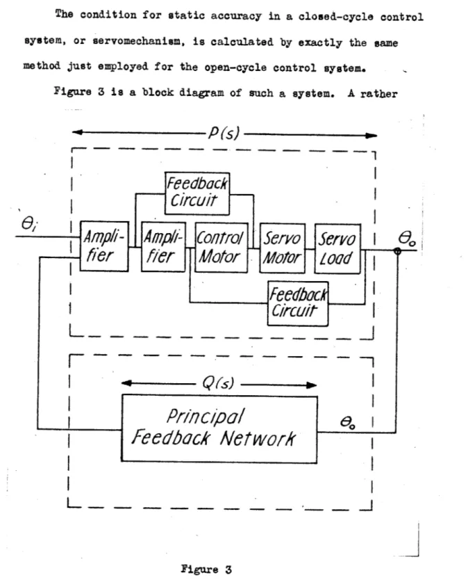
The condition for static accuracy in a closed-cycle control system, or servomechanism, is calculated by exactly the same

method just employed for the open-cycle control system. Figure 3 is a block diagram of such a system. A rather

P(s)

|

Feedback

~Circult ~~

--

-

n

Sero Saw

\

-0

fl

ie

Motor

Motor

~

0601

feecback

CIrcull

Principal

G

feedback /etwork

complex system is illustrated for the sake of generality and is divided into two components according to the dotted line enclosures.

-20-If the transfer-function (in the forward direction) of the upper enclosure is P(s) and that of the lower enclosure (in the reverse direction) is

Q(s),

00(s) = F(s)[e (s) + Q(s)& (s). (19)

Equation (19) can be written

(s) P~s9 (s -. (20)

1 - B(s)

_Q

If99 (t) is a unit function, as illustrated by Figure 2, the

transform of the servo output is

(3)

s l1 - P(s)Q(s).

The final value of,a (t) is

lim th = lim it av (22)

t -+ 01 s 1-Ps (s)

If the servomechanism is to have no static error, the following restriction must be maintained.

lim P(s) =

1

s+0 1 - P(s)

Q

Cs)

Solving,

lim Q(s) = li m - F(s)- (23a)

s-+0 s-+0 P(s)

the quantity _{lim P(s) should be as large as possible. It is}

s+0

shown in a following chapter that this quantity can be made in-finite, which is, of course, highly desirable, since in that case finite changes in its value, caused by external factors,have no effect. Equation (23a) shows, that if this function is infinite, the value of the transfer-function of the principal feedback path at zero frequency must equal negative unity in order to at-tain sero static error. Thus the following two conditions should be maintained in the closed-cycle controller in order to secure zero static error:

lim P(s) = Go a-* 0

(24)

lim

Q(s)

=

-1

The second requirement of (24), namely, that the zero-frequency value of the transfer-function of the feedback path equal a constant, must be maintained under all conditions if the static error of the system is not to vary from zero. Although it is impossible to secure a physical device with no variation in its transfer-function, the power level of the feedback path is such (it supplies signals from a

_bigh-

elec-trical and mechanical properties that the transfer-function of the feedback path approximates the required value for long

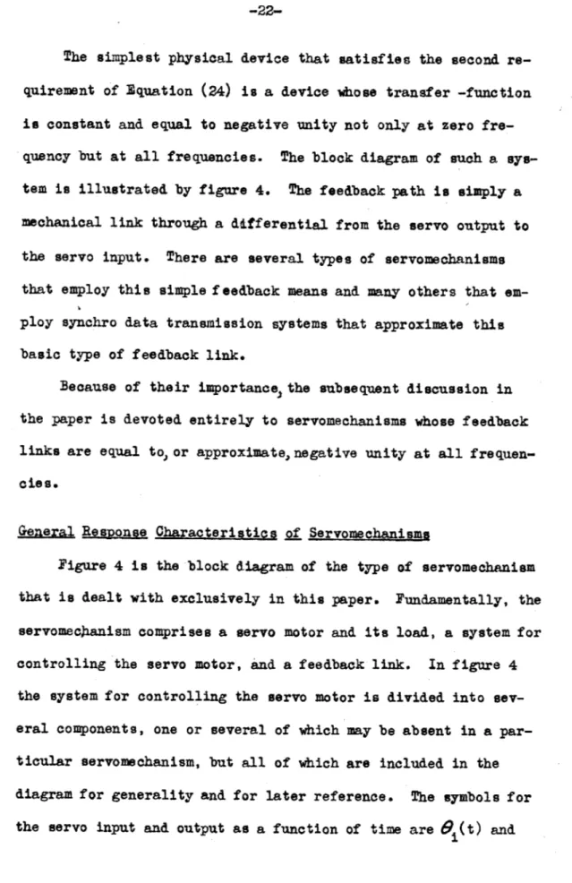
-22-The simplest physical device that satisfies the second re-quirement of Equation (24) is a device whose transfer -function is constant and equal to negative unity not only at zero fre-quency but at all frequencies. The block diagram of such a sys-tem is illustrated by figure 4. The feedback path is simply a mechanical link through a differential from the servo output to

the servo input. There are several types of servomechanisms

that employ this simple feedback means and many others that em-ploy synchro data transmission systems that approximate this basic type of feedback link.

Because of their importance, the subsequent discussion in the paper is devoted entirely to servomechanisms whose feedback

links are equal to, or approximate, negative unity at all

frequen-cies.

General Response Oharacteristics of Servomechanisms

Figure 4 is the block diagram of the type of servomechanism that is dealt with exclusively in this paper. Fundamentally, the servomecianism comprises a servo motor and its load, a system for controlling the servo motor, and a feedback link. In figure 4

the system for controlling the servo motor is divided into sev-eral components, one or sevsev-eral of which may be absent in a par-ticular servomechanism, but all of which are included in the diagram for generality and for later reference. The symbols for the servo input and output as a function of time are 19(t) and

POpO/of0/1H

CotIro/

Servo

SrVO

A///e/

Mo/or

Mo/or

ZOOd

Bas/c

Port/O? of

y51steM

Feedback L/ik-\

o 6g

SteGd'-S5atc

Error

CO/JpensJ'r

Error

CoMpe7Wtor

ConpeasOting

COnVro//er

I

-24-6

(t),

functions are defined by Equations (9) and (10). In addition, a third term is introduced which is the difference between the servo input and output mdisknown as the servo error. Its symbol is c(t), and its Laplacian transform is E(s).

C((t) 9)- (t) (25)

XEc(tU

=

E(s)

The Laplacian equivalent of Equation (25) is

E(s) =@(s) -@(s). (27)

i 0

The response of the servomechanism is completely specified by prescribing the transfer-function of the system.

KG(s) = G (28)

E(s)

The transfer-function KG(s) is the product of two functions. one that is invariant with frequency and represented by the

symbol "Y", and another, that is frequency dependent and is rep-resented by G(s). The term "K" is known as the gain factgr

or simply the gain of the system.

The Laplacian expressions for the output and error are found from equations (27) and (28).

E(s) = 1 S(s) (29)

(s)= KG(s) (s) (30) 1

+ KG( s)

Equations (29) and (30) are the defining equations of the servo system and both the transient response and the steady-state

re-sponse of the servo can be calculated from these equations. The

procedure involved in calculating these responses is outlined below.

Suppose it is desired to test the servomechanism by obtain-ing its response to some type of transient input. The general procedure to be followed in calculating either the servomeghanism

error or output is (1) determine the Laplacian transform 9 (s) of the particular input function to be applied to the servo,

(2) substitute this expression in Equations (29) and (30) and

(3) obtain the inverse transforms 19(t) and c(t) corresponding to the expressions obtained for ((s) and E(s). A common test

input is an instantaneous change of unit magnitude in the input displacement as illustrated in figure 2. The equation for this type of input function is given by Equation (12) and its Laplacian transform by Equation (13). The Laplacian transforms of the

output and error functions are found by substituting Equation (13) into Equations (29) and (30).

zi(s) =

1

__

(31)

1 + KG(s)

s

e (s) = KG(s)

1

The time responses cl(t) and t9 (t) are determined by finding

01.

the inverse transforms of Equations (31) and (32). The process involved is outlined briefly for the case of the output function.

The determination of the inverse transforms of Equation (32) is simplified if the right-hand side of the equation is expanded as a partial fraction. This is always possible for a particu-lar physical system since for such a system Equation (32) will be a rational function.

(S) = A + Al + A + + . . .(33)

9 _{a + a, s +}

a2 s + a₃

The terms a₁ , aa , a3 , etc., are the negatives of the roots of

the equation

1 + KG(s) = 0 , (34)

known as the characteristic equation of the system, and the terms Ao , A, , A , A3 , etc., are known as the residues of the

functione (s) at its respective poles. The simple form of

Equation (33) permits the inverse transform of (s), which is

01

(t), the output of the servo as a function of time, to be

found at once. It is given by Equation (35).

S(=A

Ct)

01 0

A"%l aat A &a ₃ t 11etc. The transient

transient terms Ale , A 3

real numbers or complex numbers with positive real parts. The condition that mist be met if the steady-state servo output is to be equal to the input has been considered on p.Z. If this condition exists, the steady-state term, A₀ , of Equation (35) is equal to unity, and the steady-state error consequently is equal to zero.

The character of the roots of Equation (34) (the exponents -a, , -a₂ , -a3 , etc.) and the residues A, , A2 , A3 etc.,

deter-mine the manner with which the servo output

0

_Ct)

its final value. In the ideal case the residues A, , A₂ , A₃ ,

etc., would be zero or the exponents a] , a₂ , etc.,-would be

infinite, and the servo output would follow the input instantly. Such a system is physically unattainable and the best that can be done is to so design the system that the output approaches its final value sufficiently rapidly that reasonable application requirements are met. Typical servo response curves are illus-trated in figure 5. Curve A is the response of a system all the roots ( -as , .-a2 , -a3 , etc.) of which are real and unequal;

such a system is said to be "overdamped." If the roots of the characteristic equation (Equation (34)) are all real and equal,

the system is said to be "critically damped" and the response is

illustrated by Curve B of figure 5. Complex roots give rise to responses such as are illustrated by curves C and D of figure 5

Curve

A

Ovcrdcf/pc'

Sys5/6

Curi'e

B

Crf/7//

7/ape

Systez

Curve~ C)

₇

Cufe

vJ

Sgst/C1s

9(L)

0

2

Jigure 5

and the system is said to be "underdamped." The amount the servo

output "overshoots" its final value is an inverse function of

the magnitude of the real part of the complex roots. Thus curve D is the response of a system the complex roots of which have

smaller real parts than those of the system the response of which is illustrated by curve C.

Certain requirements must be met by the roots -a, , -az -a3 , etc., in order that the servo performance be satisfactory.

Those roots that are real must be sufficiently large that the factor e-at _{0 is negligible at the end of a time interval t0}

determined by the servo application. Those exponentials that are

-28-complex must have a sufficiently large real part (damping constant)

that they, too, are negligible after the prescribed time interval,

t . A "fast" servo is characterized by large real roots and

complex roots whose real parts are large. The residues Al , A2, etc., also affect the speed of the system but not so greatly as the roots of the characteristic equation. Figure 5 shows that in general fastest servo response is obtained provided the system is so adjusted that it is slightly underdamped. Brown6

has con-sidered the transient response of servomechanisms in some detail and has given adjustment criteria for simpler systems that result

in rapid servo response.

The steady-state response of the servomechanism is also of

value as a guide to proper system adjustment. The relative

mag-nitude and phase of both the servo error and tie servo output are found from Equations (29) and (30) by replacing the complex vari-able, s, by the frequency, jw. This process has been explained

on p.1S. ___) =(36)

i1

(jw)

Valuable information is gained by studying the phase and magni-tude of both Equations (36) and (37) but at this point Equation (37) alone is considered. The functions to be examined are (1)

-30-the magnitude ratio,

Q

arcf9 (jw)J - arcfei(jw)j , (where "arc" signifies"the angle of ) of the servo output and input. Similar functions exist for the

seribmechanism error.

An ideal servo is characterized by amplitude and phase

functions illustrated in figure 6 in which the amplitude function is unity, and the phase function is zero for all frequencies.

Amplitude IResponse

=Un

ity

Phase

Response

Zero

0

_C)

---Figure 6

Such a system cannot be physic&314 obtained; however, every opera-tive servomechanism will have amplitude and phase functions which approximate the ideal over a limited frequency range. The prob-lem is to make the approximation good over a sufficiently wide

frequency range that the requirements of the application are met for which the servo is intended.

The correlation of the amplitude and phase response of a servo with application requirements such as speed of response and

6 .1

/

0

_C')

-90'

amplitude response peak is a function of the real part of the complex root. If the real roots and the complex roots of the characteristic equation are to be large and have large real parts respectively, the peaks in the amplitude response function

must be limited in magnitude and occur at large frequencies.

It has been found by experience that the real part of the root is sufficiently large if the peaks in the amplitude response are limited to approximately one and one-third. With this restriction

correlation is simplified by relating the sinusoidal response to

the transient response. _{The amplitude and phase response of a} physical servo are illustrated in figure 7. Peaks in the amplitude response generally indicate the presence of complex roots of the characteriitic equation whose complex parts correspond to the frequencies at which these peaks occur. The height of the

-32-upon the amplitude peak, the "damping ratio" of the root, as defined by Brown, _{is approximately 0.5 to 0.8, and the} imagin-ary part of the root is equal to the angular frequency at which the amplitude peak occurs within about twenty per cent. This correlation permits a rough calculation of the speed of response

MINIMUM INTEGRAL-SQUARED-ERROR SERVOMECHANISM RESPONSE CRITERION

In general it is difficult to set up and apply precise mathe-matical criteria for optimum servomechanism performance because of the individual nature of each servo application and the com-plexity of exact criteria. However, the optimum set of adjust-ments for a servo designed for any application will, in general, fall within a range that is fixed and can be predicted with fair

accuracy. _{While the accuracy and speed of response requirements}

are prescribed entirely by the individual servo application, the damping constants of the roots of the characteristic equation should all lie within a well-defined range for most servo appli-cations. The requirements of individual servo applications may best be met by particular values of damping constants, but, in general, these particular values are not widely separated.

Therefore, ideal adjustments for one servo application are close to the ideal for another application, and a servomechanism re-sponse criterion developed for a particular servo application is useful as a guide to proper servo adjustment in other problems.

A less complex mathematical criteria to set up and apply is based upon the time-integral of the square of the servo error produced by _{a particular servo input distanbance. Wor example,}

if in figure 8 curve A is the time plot of an instantaneous or step-displacement in the servo input, ti(t) , and curve B is a

-34-CurveveA

carvecc

Figure 8

possible time-plot of c(t), the resulting servo error, the

func-tion &(t)j 2 is curve C of figure 8,and the total area bounded by curve C and the time axis (the shaded area of figure 8) is a

measure of the speed of response of the system. The value of this area, denoted by the symbol, I, is expressed mathematically by Equation (38).

S=

j

[e:c(t)J

dt

(38)

This criterion is applied by so determining the adjustable

parameters of the servomechanism that the quantity, I, is a mini-mum.

The first step in applying the criterion is to express the quantity, I, in terms of the servo constants. The necessary

calculations can be performed in two ways: (1) by expressing the Laplacian transform of the error in terms of the system constants,

determining the corresponding equation for the servo-error as a function of time, and finally performing the time integration of

the square of the error as indicated in Equation (38); (2) by calculating the function, I, by integration in the complex plane. The first of these two methods is straightforward; the second is less obvious and its theory is therefore developed below.

Let c(t) equal the servo error resulting from an arbitrary input function,

0

i

of the function

0

i i

provided by Equation (29):

(

=

®

(s)

(29)

1 + KG(s)

Since KG(s) , the transfer-function of the system, can be ex-pressed in terms of the system parameters, and since the inverse transform, c(t), of E(s) can be found, a relation between the

system parameters and the time response, c(t) is derivable. The following theorem in Laplacian transform theory is di-rectly applicable to the calculation of I.*

-36-I f

_{111(s) =f fi(tg}

Then [fl(t) f

'(tJ

2r~j C2-jdo

The operation indicated by Equation (39) is a line integration in the complex plane along a line displaced c2 units to the right

of tie imaginary axis, where c2 is just large enough to avoid any

singularities lying on the imaginary axis. The function Fi(w) is the function Fl(s), with the complex variable, s, replaced by the complex variable of integration, w.

Equation (39) can be applied to the problem of calculating I.

(t) 1 c2+j E(w) E s-w) dw (40)

A second theorem in Laplacian transform theory is useful here:*

fff

(t) dt

)

+

(

dt =-0+

s s

Making use of Equation (41) and realizing that the second term on the right hand side of Equation (41) must be zero,

LJc(t)

J

s 2Se

For the last step in the calculation, use can be made of the

initial and final value theorems of Laplacian transform theory.*

Lim f(t) = lim sF(s) (43)

t-+0 s -00

Lim f(t) = lim sF(s) (16)

t+00 S-9

Then

J

sILJ

ct

s-1-0 S -+Ob

(44) Finally, since the value of

fj(t)

a

follows that Lim sdYe (t)J2 dtj= 0.

S Ce*

Therefore,

C2+jCO

I = Lim

L

s-t0 2rTj

c2-jI0

By complex variable theory,**

Jca+jO

c-00

in which JR represents the sum of the residues at the poles of

the function Fh(w) E(s-w) in the left half of the complex w plane.

Thus Equation (45) becomes

I = Lim 2 R (47)

80

Example: Type I Servo

The procedure that is followed in calculating the area under

the error-sqtared curve is clarified if an example is carried

* See reference 9 , p. 265 and 267. ** See reference

26,

113

--4

-38-through. A simple system that is often employed to demonstrate design principles comprises a servo motor whose load consists of moment of inertia, J , and viscous damping, f , and whose

torque is directly proportional to the error. Such a system, termed a type I servo by Brown,6 _{is illustrated by figure 9.}

TYPE

1

SERvo

SProp

orfiori

U

T

Servo

s

o

C017M11Crmotor

G117

= kP

Servo

This servo is discussed in more detail in the discussion begin-ning with p.I56 . At this point it will be employed as an example to illustrate the calculation and application of the criterion

just developed.

The Laplacian expression for tue error of this system is given by Equation (48).

i(s) =

Ls

+ 1)

(s)

(48)

TL(82 + _ + kP

L L L In the above equation,

k = torque - error constant of the system (torque developed

I

by the servo motor per unit of error.)

JL = moment of inertia of the load and rotating parts of

the motor.

f = viscous damping acting upon the motor output.

TL L

If the input function,

9

trans-form,

e.(s),

squared-error curve may be calculated by Equation (47) and is found to be

I =

s-+0 _{f+p + L (s-w)+ -w +T}

L .L L L L

(49)

in which R signifies "the sum of the residues in the left half plane." The residues occur at the roots of the

charac-teristic equation.

W + w + p ='0

L L L

These roots are

w=-1 Ll +1-.A p L )J. 2T L p L Let P

L

-40-The residues are evaluated from Equation (53), derived from Equation (49): I = Lim + T w TL (s-W) +

1

JJ1

)+

the following compact form:

I= L (C+.b) (5)

2 b

Equation (48) is frequently written in the following form:

) = S(s + 2tw S2 + 2tw_{0s + W} (55)

In the above equation

'IT L

k/J =w .

(56)

(57)

The time function, c(t), is then studied for various values of

C,

held invariant. If Equation (54) is rewritten in terms of the

symbols w and , Equation (58) is obtained.*

I =

_

w 4C

It is, of course, desirable to so adjust the system constants

that I, the area under the squared-error curve, is a minimum.

Equation (58) shows that the value of I varies inversely with the

natural frequency, wo₀, provided the damping ratio, C, is held

con-stant. If t is varied and w0 held constant, a minimum value of

I occurs when the damping ratio is equal to 0.5. The resulting

value of I is given by Equation (59).

1

~(59)

Thus the criterion of minimum integral-squared-error yields the fact that the optimum value of C is 0.5 provided the natural

freauency,w0 , is constant.

However, the ratio, wo, is not a convenient quantity to hold invariant, since it is proportional to the torque-error constant, k, the only system constant easily adjusted. The

p

ratio T = L is more logically held constant since it

de-pends only upon the load on the servormotor output and is gener-ally fixed by externgener-ally imposed restrictions. A more correct consideration of the problem, therefore, is to so adjust the

con-stant, k, that a minimum value of I occurs for a given value of p

-42-T_{L. Equation (54) supplies the answer to this problem.} Since

b is directly proportional to kp, the correct value of k is

cal-p

culated from the value of b that result s in a minimum value of I. A plot of I as a function of b is given in figure 10.

- 4 . 4 4 - t - 1 FT 1

.4

VV4

4

47-

-T-

The significant fact is that I is a constantly decreasing

uIM.-jion with i

ncrasing

constant, ) , is iainite. Obviously, such a conclusion is errone-p

ous for any physical system. The reason such a result appears is that the simple system of figure 9 is stable for all values of )E although very large values of k produce a very low damping

ratio. The natural frequency, w0, increases as iC is increased,

however, and at such a rate as to overcome the result of the creasing damping ratio and to result in the variation in I de-picted by figure 10. Actually, no physical system exists that is stable for all values of gain and there is always a finite optimum value of gain for every physical system. The fact that

I decreases constantly with increasing values of gain is an indi-cation that for certain purposes the type I servo is an invalid approximation for a physical system. This point is discussed

again in Chapter VI.

xamle: Third-Order Servomechanism

The response of a physical servo system is much more accu-rately represented by an expression for E(s) orSo(s) of the third order than of the second order. A system whose character-istic equation is of the third order will always become unstable if the gain of the system is increased indefinitely, and therefore, the fallacy of a constantly decreasing integral I with increasing gain will not be encountered. It is of interest, therefore, to determine the conditions under which the integral, I, is a minimum for the case of the third-order system.

The transform of the error of a third-order system can gen-erally be written

E(s) S(82 +

ea

(s)

Equation (60) is general for all servo 4ystems that have no positional error (see p.6-) and thus applies to practically all systems of interest. Because of the relation between the numera-tor and denominanumera-tor of Equation (60), specification of the roots of the characteristic equation (the denominator of Equation (60)

equated to zero) completely determines the system response. Let -the three roots be known as X3, X₂ , and X . Since the product of

the three roots is r,

%I X2 X3 = r, (61)

the roots can be written as

X= a L (62)

Xa = a (63)

X r[ 0 ₍₆₄₎

a2

-In the above three equations, advantage is taken of the fact that optimum performance is secured if the roots are complex in char--acter, and that in a third-order-system at least one root must be real. Therefore, a is the magnitude and the angle of the complex roots.

The expression for I, the area under the squared-error

curve, may be found by one of the two methods outlined previously. The actual calculation although straightforward is laborious. The work is not repeated here but the final result is given by Equation (65).

1=

_.1.

_e

D2 a3 r a3Cosa

+ 8Aaar sinGi sin(b -6-

y)

B

2a

sin/

ja

cos

- a

tan'l

a

sin

'

sin

cosG

The complete determination of the mathematical minima of the quantity I is unsolved. It is possible to show that one minimum exists whenO equals zero and a = ; that is, the function I possesses a minimum when all the roots of the charac-teristic equation are real and equal. Although other, and

smaller, minima exist when the roots of the characteristic equa-tion are complex, the mathematical condiequa-tions for their existence

have not been found. The approximate determination of the minima

(65)

of the function, I, has been carried out, however, by calculat-ing and plottcalculat-ing the function for various assigned values of the magnitudes and angles of the roots of the characteristic equation. These results are summarized in the curves of figure 11. It is

4

7-

----~T

I

t

-

'

-;l~G iiljii-

-

j-/250-

7-

1/

i ot

m

o

e

t

an.

te

see tha th mleto h ormnm hw cuev h

senta h

magnitud of the r o su l tiiao n 2r) r 1/ n henglhe