Analysis and comparison of metrology methods for quantifying micro-endmills

(1)

Analysis and Comparison of Metrology Methods

for Quantifying Micro-Endmills

by

Jennifer Ariel Doyle

SUBMITTED TO THE DEPARTMENT OF MECHANICAL ENGINEERING IN PARTIAL FULFILLMENT OF THE REQUIREMENTS FOR THE DEGREE OF

BACHELOR OF SCIENCE IN MECHANICAL ENGINEERING AT THE

MASSACHUSETTS INSTITUTE OF TECHNOLOGY

June 2009

in whole or in part in any medium now known or hereafter created.

MASSACHUSETTS INSITUTE OF TECHNOLOGY

SEP 16 2009

UL BARIES

/

De rtmef of"'/' - z

Jennifer Ariel oyle anical Engineering May 18, 2009 Certified by: _j

Accepted by:

/ / Martin L. Culpepper

A te Professor of Mechanical Engineering

Thesis Supervisor

John H. Lienhard V lins Professor of Mechanical Engineering Chairman, Undergraduate Thesis Committee

(2)

(3)

Analysis and Comparison of Metrology Methods

for Quantifying Micro-Endmills

by

Jennifer Ariel Doyle

Submitted to the department of Mechanical Engineering on May 18, 2009 in partial fulfillment of the requirements for the degree of Bachelor of Science in

Mechanical Engineering

Abstract

Micromilling is a powerful machining method increasingly used in the medical, optical, and electronics industries to rapidly create 3-dimensional, micro-scale components for meso-scale devices. The micromilling process causes higher incidences of tool wear and breakage, which are often not readily visible on micro-scaled tools. However, these tool defects must be accounted for if the process is to be made reliable. Size differences on the order of tens or hundreds of microns may be negligible in macroscale or "conventional" milling, but in micromilling it is not uncommon for the workpiece to be on the order of this size. As such, accurate, repeatable tool metrology is necessary for successful micromilling. This thesis presents a summary of four micro-tool metrology methods, relating qualitative measures such as ease of use, image quality, and tool throughput as well as the numerical validity of tool measurements obtained by the four methods. This was achieved by measuring the diameters of ten micro-endmills of five different sizes; each endmill was measured using all four measurement techniques. A Microlution 363-S series micromill, which uses a laser-occlusion measurement system to confirm tool geometry, was found to be simpler and faster than optical, digital, and scanning electron microscopy methods. Though laser occlusion lacks the visual information provided by microscopy, calculated Student t-test p-values for this method were greater than a set 0.1 significance level for every tool size. All three microscopy methods had p-values below the 0.1 significance level for some tool sizes, suggesting that the laser occlusion method provides the lowest statistical likelihood of variance in measured tool geometry due to measurement error. Furthermore, all four measurement techniques were found to be more accurate when measuring smaller tools than when measuring larger tools; in particular, SEM measurements of large tools suggested a high probability of incorrect measurement. The findings presented here have the potential to foster further discussion and use of on-machine measurement systems in microscale metrology over the currently prevailing microscopy methods, in particular SEM.

Thesis Supervisor: Martin L. Culpepper

(4)

Acknowledgements

I would like to thank first and foremost Professor Culpepper for selecting me to participate in the MIT-Lincoln Lab Beaverworks project. It was not always an easy path, but I have learned incredible lessons which I would not have learned in any other

class, through both the successes and the failures of this project.

Thanks goes out to all of the Beaverworks team, in particular: Alex Slocum, Jr., for helping me find my way on this thesis project despite some initial struggles. Also, I would like to thank Dan Lorenc and Aaron Ramirez for their nonstop, late-night efforts with me on the micromilling machine. Writing G-code late at night is not the same without a friend!

I would like to give a special thanks to the engineers at MIT's Lincoln Laboratory who accommodated me and my metrology research, giving much of their own time and tons of invaluable advice over the past few months. In particular, I would like to thank George Haldeman, David Ruscak, Christine Wang, and Saunak Shah. I hope that my research and experiences with the Keyence microscope can be of use to the Lab in the future.

My sincerest thanks also goes out to others at MIT who assisted with measurements, specifically Pierce Hayward in the AMP Laboratory on the optical microscope and Mark Ralph in the Pappalardo II Laboratory with the scanning electron microscope.

Finally, I would like to thank my friends and family. Special thanks to Karina Pikhart, for her endless support over the last semester and past semesters - I could not have made it through Course 2 without her infinite amount of encouragement. Thank you to my twin brother, Brian, for his last-minute assistance on data analysis and editing, as well as his upbeat outlook.

To everyone above and to those who I have somehow forgotten to mention, thank you for your help and support.

(5)

List of Figures

2.1: Illustration demonstrating the minimum chip thickness effect [4]. ... 12

2.2: Comparison of tool size versus grain size in macroscale milling (left) and micromilling (right) [7]... ... 13

3.1: The Microlution 363-S micromilling machine. ... ... 18

3.2: The tool, spindle, and palette in position during a laser measurement sense ... 19

3.3: The first image taken using the digital microscope - the side view of a 0.0050" diameter endmill, shown under 1000x magnification ... ... 21

3.4: 3-dimensional digital image of the tip of a 0.015" 2-flute diameter endmill, magnified 500x. Color contours provide height information. ... ... 22

3.5: Point-to-point measurement of a sample 0.005" diameter endmill, measuring from flute tip to flute tip. The large size of the green point selectors yielded variable results, resulting in the switch to a different image analysis method ... 22

3.6: When zoomed in on this SEM image of a 0.015" diameter tool, it is possible to see the amount of pixelation that makes it difficult to select the "true" tool edge; thus, high and low estimate values are taken from each image ... 25

4.1: Tool A, a 0.005" diameter endmill, imaged under optical microscope. ... 28

4.2: Tool A, a 0.005" diameter endmill, imaged under scanning electron microscope ... 29

4.3: Tool A, a 0.005" diameter endmill, imaged under digital microscope. Note that scale in this image is incorrect and should actually be half the values shown ... 29

4.4: Tool B, a 0.005" diameter endmill, imaged under optical microscope. ... 30

4.5: Tool B, a 0.005" diameter endmill, imaged under scanning electron microscope ... 30

4.6: Tool B, a 0.005" diameter endmill, imaged under digital microscope ... 31

4.7: Tool C, a 0.015" diameter endmill, imaged under optical microscope. ... 32

4.10: Tool D, a 0.015" diameter endmill, imaged under optical microscope. ... 34

4.11: Tool D, a 0.015" diameter endmill, imaged under scanning electron microscope...34

4.12: Tool D, a 0.015" diameter endmill, imaged under digital microscope ... 35

4.13: Tool E, a 0.020" diameter endmill, imaged under optical microscope. ... 36

4.14: Tool E, a 0.020" diameter endmill, imaged under scanning microscope ... 36

(7)

4.16: Tool F, a 0.020" diameter endmill, imaged under optical microscope...38

4.17: Tool F, a 0.020" diameter endmill, imaged under scanning electron microscope ... 38

4.18: Tool F, a 0.020" diameter endmill, imaged under digital microscope ... 39

4.19: Tool G, a 0.040" diameter endmill, imaged under optical microscope. ... 40

4.20: Tool G, 0.040" diameter endmill, imaged under scanning electron microscope. ... 41

4.21: Tool G, 0.040" diameter endmill, imaged under digital microscope...41

4.22: Tool H, a 0.040" diameter endmill, imaged under optical microscope. ... 42

4.23: Tool H, a 0.040" diameter endmill, imaged under scanning electron microscope. ... 43

4.24: Tool H, a 0.040" diameter endmill, imaged under digital microscope. ... 43

4.25: Tool J, a 0.125" diameter endmill, imaged under scanning electron microscope. ... 44

4.26: Tool J, a 0.125" diameter endmill, imaged under digital microscope. ... 44

4.27: Tool K, a 0.125" diameter endmill, imaged under scanning electron microscope...45

4.28: Tool K, a 0.125" diameter endmill, imaged under digital microscope ... 45

5.1: The 0.040" diameter endmill broken during machining the tool wear slot sample. Most broken tools split at an angle rather than parallel to the plane of the tip... 50

5.2: Correct positioning of endmill on optical slide for true diameter measurement. Note that the two cutting tips are oriented at the upper-most and lower-most points in the Y direction, so that a vertical measurement line drawn from tip to tip measures the true diameter with no Z-component [16]. ... ... 52

5.3: As the positioning of the two endmill tips rotates away from being vertically aligned with the Y-axis, a Z-axis component of the diameter is introduced that is not visible from the microscope view direction, potentially skewing diameter measurements [17]. ... ... 5 2 5.4: A misaligned 0.005" diameter endmill, misaligned (left) and correctly aligned (right). 53 5.5: Top, a completely horizontal endmill, such that the vertical length measurement from tip to tip correctly measured the diameter. Below, an unaligned endmill with an incorrectly measured diameter... ... ... 54

5.6: On the left, the 0.015" diameter endmill with its upper tip in focus and its lower tip out of focus; on the right, the same tool and image, but with the focus shifted to the lower tip . ... ... 5 5 5.7: Tool D, a 0.015" diameter endmill, has its shaft more in focus than its tip, which caused difficulty in im age processing ... 57

(8)

5.8: The image of tool F, a 0.020" diameter endmill, is almost completely dark on its left side. ... ... 58 5.9: A 0.010" unused diameter tool, which appears to have dark pockets and shadows on the right h alf. ... ... 59 5.10: A rotated and color contoured version of Fig. 5.9 demonstrates that what appeared to

be pockets are actually raised areas. ... 60 5.11: The cleaned 0.010" diameter tool tip now shows little evidence of damage or wear. ... 61

List of Tables & Charts

3.1: Tools purchased from Performance Micro Tool with corresponding dimensions... 16 4.1: Measurements of ten tools using the milling machine laser sensing and the optical

microscope. All values are in microns ... ... 46 4.2: Measurements of ten tools using the scanning electron microscope and the digital

microscope. All values are in microns ... ... 47

(9)

Analysis and Comparison of Metrology Methods for

Quantifying Micro-Endmills

Chapter

1 Introduction

This thesis was conducted as part of a larger group project hosted by the MIT Precision Compliant Systems Laboratory and sponsored by MIT's Lincoln Laboratory. One specific aim of the project was to investigate the capabilities of micromilling as a rapid prototyping process. The research activities undertaken in this aspect of the project were framed within the context of designing and fabricating a prototype metering valve for a micro-power generator for further use by Lincoln Laboratory.

One of the goals set by Lincoln Laboratory was to compare micromilling with other modes of manufacturing at the microscale, for example microlithography and etching, to assess the capabilities of micromilling for rapid prototyping. Comparisons can be made between process parameters such as cost, rate, quality, flexibility, repeatability, feasibility, and size and shape limitations of each of these micro-manufacturing methods. Preliminary research into a variety of micro-micro-manufacturing methods was undertaken in the first stage of this project. From this it was determined that although microlithographic processes may be superior for mass fabrication and production, micromilling is one of the most efficient processes for conducting rapid prototyping of microscale designs, such as the microscale metering valve design used as the case study by this project group.

Within the context of the project discussed above, the original purpose of this thesis was to more thoroughly investigate and experiment with micromilling, in order to develop Design for Manufacturing (DFM) guidelines for when using micromilling for prototyping. In addition, it was expected that although micromilling would be used in the prototyping stages of the design process, lithographic processes would be implemented in later bulk production stages. As such, it was essential for such DFM guidelines to map features created using micromilling to lithographic processes capable

(10)

of creating those features as well. Following these guidelines would allow a design to be manufacturable both by micromilling and by lithographic methods.

The initial plan for developing DFM rules for micromilling was to machine various features like holes, slots, and pockets, within a wide variety of aspect ratios

-pocket depth to width/length, for example. These features could be measured; the accuracy and repeatability with which each feature was created, as well as the feasibility of creating each feature, would then be recorded. In order to obtain suitable numerical data, however, it was necessary to confirm the geometry of the tool used to create each feature both before and after machining. It became apparent that obtaining useful and usable qualitative and quantitative information about these tools is a far more complex and time consuming problem than initially assumed.

Due to the inadequacies encountered in the tool measurement methods, this thesis evolved from its original concept into one examining microscale tool metrology.

Although creating DFM guidelines for micromilling is important - and may certainly be

undertaken at a later time - it was thought that the issues with tool metrology must be

resolved before a high-quality development of DFM rules could be attempted. As such, the ultimate goal of this thesis was to analyze different methods of measuring specific parameters of micromilling cutting tools. This would be done to both establish the advantages and disadvantages of each method and to determine if any one method was most applicable for micromilling.

It was hypothesized that there would be no one "correct" method of measuring tools on the microscale. Certain metrology methods may produce better qualitative images but lack suitable means to process those images; other methods may produce higher quantitative accuracy and repeatability yet require greater training or setup time to use them, and thus not be economically feasible from a rate and flexibility point of view. However, it was expected that the qualitative and quantitative analysis undertaken in this project would help elucidate the comparative merits of each method, making it easier to select a relatively superior method of microscale measurement for use in the future.

(11)

Chapter 2 Background

2.1 Motivation for Micromilling

The increasing trend towards miniaturization in such fields as electronics, telecommunications, medicine, biotechnology, and optics has increased the need for reliable ways of producing microscale components. These components, such as micro-sized fuel cells, pumps and valves, nozzles, masks, and molds, consist of complex 3-dimensional features ranging in size from a few microns to a few hundred microns. For example, according to Vogler et al., parts with lengths and widths of no larger than 500 microns, wall thicknesses of 25-50 microns, and holes 125 microns in diameter are not uncommon in current applications [1].

Due to the proliferation of microcomponents over the last several years, development of new microscale manufacturing methods has also increased. Many of these microfabrication methods are lithography based, such as wet etching, dry etching, plasma etching, and surface machining, and have been put to use in the creation of microelectromechanical systems (MEMS) devices. While these methods are perhaps appropriate in the fabrication of MEMS, they have their limitations. Lithographic methods are primarily focused on using silicon or silicon-like materials [2], which may be appropriate for certain applications or for final production runs but due to cost may not be suitable for use during the prototyping process. When using lithographic techniques, features are produced in a single plane; creating 3-dimensional structures requires layering that is once again costly as well as time consuming. In contrast, 3-dimensional features can be machined in a single operation using microscale machining. Compared with the monetary expenses of manufacturing exposure masks and the time costs of lithographic layering, micromilling offers a more viable means of creating single parts and prototypes or small batches of components [3].

2.2 Working at the Microscale

Micromilling is, in both principle and execution, similar to macroscale milling, but there are major differences in the underlying physics due to the process being

(12)

miniaturized in scale. In conventional, macroscale milling, the characteristic thickness of chips produced are generally at least an order of magnitude greater than the edge radius of the cutting tool. However, the edge radii of cutting tools used in micromilling are comparable in size, or even slightly larger than, the micromachined chip size. As a consequence, in micromilling, no chip forms when the chip thickness is below a minimum value, or trmin. When the chip thickness is below tmin, the part of the workpiece under the edge of the tool plastically deforms, while the rest of the material elastically recovers. This ploughing- and rubbing-based elastic-plastic deformation is known as the minimum chip thickness effect, and is shown visually below in Fig. 2.1.

Chip / Tool

ToolTl

C / F

B A t

(a) (b)

Figure 2.1: Illustration demonstrating the minimum chip thickness effect [4].

Unlike in macroscale milling, where the cutting process is dominated by chip formation, in micromilling, the process frequently switches between the mechanism of shearing and chip formation and this mechanism of ploughing and rubbing [5]. In fact, the cutting mechanism may switch between ploughing and shearing even within a

single cut from flute to flute [2].

In addition, when machining on the microscale, desired part geometries and the grain sizes of common workpiece materials such as steel and aluminum are on the same

order of magnitude - between roughly 100 nm and 100 microns. This results in the

microstructure of the workpiece material playing a much larger role than in macroscale

milling, as many workpiece materials - even commonly-used materials such as steel

-can no longer be considered homogeneous, as demonstrated in Fig. 2.2 below. In macroscale machining, a single cut likely passes through several grains. Conversely, in micromilling, the cutting tool may be completely contained within one grain while cutting [6].

(13)

V V

>->, Tool

Figure 2.2: Comparison of tool size versus grain size in macroscale milling (left) and

micromilling (right) [7]. _{The individual grains, in this case shown as interlocking}

triangles, are delineated by the red lines.

2.3 Tool Wear

These two major differences - the introduction of the minimum chip thicknesses

effect and the grain size effect - _{are frequently discussed in the literature and have}

been shown to impact surface finish and quality, particularly with respect to burr formation [2]. However, the most important reason to address these phenomena in this project is because of the increased risk of tool wear and tool breakage. Switching between the shearing/cutting mechanism and the rubbing/ploughing mechanism can increase cutting forces [5]. The movement of the cutting tool between grains of a material and from one phase to another also creates significant variations in cutting forces; furthermore, there are accounts of significant workpiece excitation when crossing grain boundaries [6]. Increased cutting forces and the resulting vibrations lead to accelerated tool wear [1]. In addition, when increased cutting force and tool wear are combined, stresses occur in the tool that surpass the yield strength of such micromilling tools, leading to tool breakage -often quite rapidly after initial onset of wear [8].

Because of the small size of micro cutting tools, tool wear and even breakage are not easily visible to the naked eye. Thus, the macroscale methods of observing tool breakage or even hearing tool breakage are not applicable, and new methods of detection are necessary. Tool wear and breakage must be recognized and accounted for, since part geometry and accuracy are directly dependent on the accuracy of the tool. While size differences and wear on the order of tens or hundreds of microns may be negligible on the macroscale, at the microscale this cannot be ignored. Along with the expectation that there will always exist some variability between manufactured tools of

(14)

the same size, this makes tool metrology a necessity for accurate and repeatable micromilling.

2.4 Current Micro-Metrology Methods

Currently, the scanning electron microscope, or SEM, appears to be the most common tool of investigation used in assessment of micromilling. For example, in a study of chip formation during micromilling, Kim et al. collected chips and examined them using an SEM in order to estimate chip length, width, and thickness [9]. Lee and Dornfeld qualitatively measured burr sizes using an SEM in their examinations of burr formation when milling aluminum and copper [10]. Moriwaki et al. investigated the impact of micromilling on chip formation along various crystallographic planes in single-crystal copper by performing experiments in situ inside an SEM [11]. Micromilling-related scratch tests conducted by Taniyama et al. were analyzed using a field emission SEM [12].

Even though SEM use is prevalent in current metrology methods, other metrology tools are also used. The details and structures of micro-scratches on different materials investigated by Jardret et al. were measured using a 3D SURFASCAN topometer [13]. Additionally, in Vogler, DeVor, and Kapoor's modeling and analysis of surface generation and quality in micromilling, the surface roughness of sample machined slots was measured using a Wyko NT 1000 optical profiler, which created a 2D grid of surface heights. However, for a further qualitative look at the impact of grain boundaries on surface effects and burr formation, Vogler et al. then imaged the

machined slots again with a SEM [6].

It is important to note that in most of the literature, metrology is often used, but the results are limited to being somewhat qualitative. In addition, almost every single mention of metrology for micromilling is in regards to measuring aspects of the machined samples, rather than measuring the working tools. When Schaller et al. shaped their own single-edge endmills using commercial metal tool grinding techniques, they admitted the difficulty of comparing tools of "equal" geometry. Rather than measuring each tool to investigate tool quality and accuracy, tools were simply judged by failure during machining tests and optical inspection of machined samples

(15)

[15]. There are few exceptions, such as in the research by Rahman et al., where tool wear was measured using an Olympus Toolmakers microscope [14].

Thus, the research in this thesis - specifically focusing on tool metrology - hopes to uncover what has been traditionally ignored by previous work in the micromilling field.

(16)

Chapter 3 Experimental Design

3.1 Cutting Tools

Cutting tools were purchased from Performance Micro Tool', a company offering solid carbide tools in micro- and nano- sized diameters. 2-fluted endmills with cutting tips 180 degrees apart were chosen in a range of diameters, listed below in Table 3.1.

Table 3.1: Tools purchased from Performance Micro Tool with corresponding dimensions.

Manufacturer's Part Tool Size (in inches) Tool Size (in microns)

Number TS-2-0050-S 0.005 127 TS-2-0100-S 0.010 254 TS-2-0150-S 0.015 381 TS-2-0200-S 0.020 508 TS-2-0400-S 0.040 1060 SR-2-1250-S 0.125 3175

Over the course of this project and the sample machining undertaken, many tools were broken, such that not all tools measured necessarily came from the same ordered batch. With the exception of the 0.125" endmills, the tools from PMT have a tolerance specification of ±0.0005" (12.7 microns). The 0.125" endmills have a tolerance of +0.000 (0 microns)/-0.002" (50.8 microns).

3.1.1 Tool Parameters

There are several properties of the cutting endmill that potentially impact whether a machined part matches the desired shape and dimensions. In order for the tool to cut slots and pockets with vertical walls, the tool shaft must be straight and untapered. Concentricity of the shaft and cutting flutes with the machine spindle is also important, as a shaft whose tip is not concentric with its base has the potential of producing eccentric holes or holes that are larger than the tool diameter. The most

(17)

critical parameter is the tool diameter. A tool whose diameter is different from expected, due to mis-production, wear, or even misidentification the tool - which could arise in micromilling due to the cutting tips being too small to be identified by the

naked eye - will most definitely produce a machined part with undesired dimensions.

It is important to realize that there are various parameters that affect the size, shape, and finish of machined parts; in an ideal situation, all of these parameters would be measured and validated before machining. However, due to constraints on resources and time, the experimental process undertaken in this paper only looks at tool diameter. It was determined that this parameter is perhaps the most fundamental; if tool diameter is not accurate, then all other process parameters are irrelevant. In addition, tool diameter is also a characteristic that could be measured in a large variety of ways. For example, the tool could be imaged orthogonal to its plane of symmetry or along its axis of rotation to obtain diameter measurements. This aspect of measurement flexibility opened the door to a larger number of metrology methods.

3.2 Measurement Apparatus

Four metrology methods were selected for this project: the built-in laser tool sensing apparatus on the Microlution 363-S milling machine, optical microscopy, digital microscopy, and scanning electron microscopy. Further discussion of each method is described below.

3.2.1 Milling Machine Laser Tool Sense

The micromilling machine used in this project was a Microlution 363-S 3-axis, CNC, horizontal milling machine, shown below in Fig. 3.1.

(18)

Figure 3.1: The Microlution 363-S micromilling machine.

This machine has a laser occlusion-based tool tip sensor that can automatically detect tool length and tool diameter. The laser is fixed to the workpiece palette. To conduct measurements, the chosen tool was clamped in the spindle, and the desired measurement option was selected on the machine's onboard computer system. The spindle moved forward to the workpiece palette, and the palette moved accordingly to allow the tool to move into range of the laser. This is demonstrated in Fig. 3.2 below. When the measurement was completed, the spindle retreated backwards and the single measurement was projected on the computer screen.

(19)

Laser

Workpiece Palette Endmill

Figure 3.2: The tool, spindle, and palette in position during a laser measurement sense. 3.2.2 Optical Microscope

A Nikon optical microscope with an attached camera was used to take images of the selected tools. The chosen tool was placed on its side on a microscope slide and fastened in place using fixturing gum. To ensure an accurate diameter measurement, the tool was aligned horizontally, using the parallel (long) edge of the microscope slide as a reference. Tools measured with the optical microscope were magnified under a 20x

objective lens, which provided a 200x view when combined with the 10x ocular lens.

The captured images were loaded into Motic Images Plus software, which contains a

length-measurement function correlated with the microscope zoom. The length function in the image viewing software was used to measure from the cutting tip of one flute to the cutting tip of the opposite flute. These measurements were recorded and the images saved for qualitative investigation.

3.2.3 Digital Microscope

A Keyence VHX-500F series digital microscope at Lincoln Laboratory was used for the next phase of the tool measurement process. One problem with using an optical microscope such as the one described above is that the depth of field is limited - the microscope can only focus clearly on a small depth range. The digital microscope solves this issue by capturing images over a range of focuses and then combining the images into a single, in-focus composite, a process known as focus stacking. This allows for a

(20)

greater depth of field and thus better viewing of a specimen with a large height

difference - a specimen that an optical microscope may not be able to focus on

adequately.

Basic operation of the digital microscope was similar to that of the optical microscope. The selected tool was placed underneath the lens and a chosen depth on the

tool - typically the lowest desired point - was brought into focus. Interchangeable

heads with varying zoom powers were available and switched depending on the tool being measured to provide the highest level of magnification possible (higher magnification heads for smaller tools, and vice versa). Starting with the lowest desired point in focus, a view range was selected on the computer by adjusting the focus until the highest desired point was clear. Once the focus range was chosen, the microscope automatically repositioned, refocused, and took images over a series of steps within the range. There was the option of guiding the stepped image process in terms of height per step or total number of images within the range. In all cases for this project, it was decided that taking 50 images of equal step size within the height range would be appropriate.

Due to the digital microscope's additional functions and the author's unfamiliarity with the device, this microscope's imaging capabilities were initially explored outside of the context of any specific experiment. Whereas image quality and depth of field made viewing tools from the side a necessity with the optical microscope, sample tools were examined with the digital microscope in a side-on position, as shown in a sample image in Fig. 3.3, as well as in a tip-on position. An attempt was made to position the selected tool at an angle in order to inspect both the tip and the sides concurrently; however, difficulties in focusing the microscope and achieving intelligible results resulted in this approach being discarded. For the most part, the tip-on view proved to be more useful for conducting diameter measurements, as it was much easier to pin-point both flute tips than when looking at the tool from the side. Thus, with the exception of a few qualitative side-on views, all images captured with this method beyond this point were taken directly viewing the tool tip. Due to limited materials at Lincoln Laboratory, tools were secured into position by inserting them into block of foam.

(21)

Figure 3.3: The first image taken using the digital microscope - the side view of a 0.005"

diameter endmill, shown under 1000x magnification.

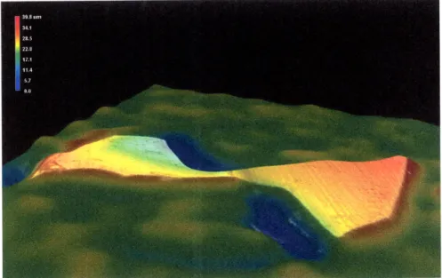
Although tools were oriented in the tip-on position for a majority of the images, the Keyence digital microscope does have the additional capability of being able to create rotate-able 3-dimensional images with height-based color contouring, as shown on another test image below in Fig. 3.4. This capability was used for qualitative analysis on some tools and was used as an alternative to side-based imaging, but was not used in diameter measurement.

(22)

Figure 3.4: 3-dimensional digital image of the tip of a 0.015" 2-flute diameter endmill,

magnified 500x. Color contours provide height information.

The Keyence software came with a point-to-point measurement system that was initially explored as a potential way of easily measuring images, similar to the method used with the optical microscope software. However, the point selectors on this software program were quite large and tended to obscure too much of the tool tips, as shown in Fig. 3.5.

Figure 3.5: Point-to-point measurement of a sample 0.005" diameter endmill, measuring

from flute tip to flute tip. The large size of the green point selectors yielded variable results, resulting in the switch to a different image analysis method.

(23)

It seemed unlikely that this would lend itself to accurate measurement. Instead, captured images were viewed in Paint Shop Pro and the pixel coordinates locations of the tool flute tips were recorded. The horizontal and vertical pixel differences between the two points were converted into a hypotenuse pixel measurement. Because the images were saved with a scale bar, it was possible to create a pixel-to-micron

conversion ratio, which was then used to translate the pixel hypotenuse measurement into a diameter measurement in microns.

3.2.4 Scanning Electron Microscope

A scanning electron microscope (SEM) was the final method used to image the

micro endmills in this project. Tools were positioned with the tip facing the SEM microscope lens, similar to the setup implemented when using the digital microscope. However, the SEM required a more specific holder for the tool specimens than the foam support used for the digital microscope. The holder needed to be electrically conducting; in addition, because of the challenges associated with unloading and reloading the SEM, it was decided to design the holder to accommodate multiple tools. A disk-shaped holder was fabricated out of 0.5" aluminum stock with 12 holes spaced radially about disk to hold the tool shafts. The holder mounted into the SEM via a computer-controlled central shaft, which allowed the disk to be rotated to change which tool was in view without opening and evacuating the specimen chamber.

Each selected tool was rotated into view, brought into focus, and then imaged. The image processing method used to calculate the tool diameter from the SEM images was the same as described above for the images taken using the digital microscope.

3.3 Experimental Procedure

To compare the four different metrology methods, a set of ten unused tools was selected for diameter measurement. The ten tools consisted of two 0.005", two 0.015", two 0.020", two 0.040", and two 0.125" diameter endmills, which were respectively labeled as tools A-K (excepting I) for convenience. Each tool was measured using the four measurement techniques, using the processes described in the previous section. Note that for future reference, the ten cutting tools themselves were typically referred to by their letter designation or their size in imperial units, as that was the unit system

(24)

provided by the manufacturer. However, the resulting measurements and analysis were conducted in metric microns; given the small size of the tools, such a scale seemed more appropriate, and all four metrology methods provided measurements or scale bars in microns.

For the Microlution laser sense method, three measurements were taken for each tool, providing three diameter values for each tool. Each image taken by the three

microscopy methods yielded two diameter measurement values - a "high" measurement

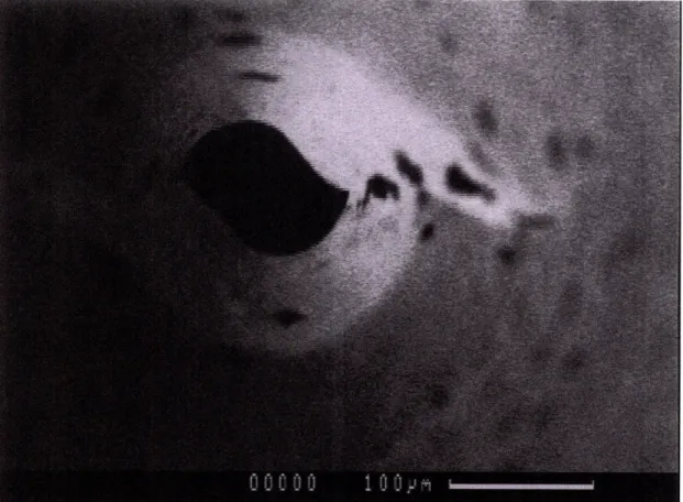
and a "low" measurement. Because the resolution and quality of images are not infinite, there must be some pixelation at the tool edges. The "high" measurement was therefore the value on the outside range of the pixelation, the "low" measurement on the inside range. This process is shown in Fig. 3.6. As can be seen in the Fig. 3.6, in some cases the pixelation was so extreme that the high and low estimates were rough estimates at best.

(25)

Low estimate

Figure 3.6: When zoomed in on this SEM image of a 0.015" diameter tool, it is possible to

see the amount of pixelation that makes it difficult to select the "true" tool edge; thus, approximate high and low estimate values were taken from each image.

Two different images were captured for each tool using the optical microscope. Two images were also taken using the SEM for each tool. In each of these two SEM

images, the positioning of the tool was the same, but one image was at a low

magnification and one image was at a higher magnification. Due to time constraints,

only one image (with its respective two estimated measurement values) was taken of

each tool using the digital microscope.

It was expected that there is some variation between tools of the same size, perhaps greater than the tolerances specified by the manufacturer. Without details

from the manufacturer, is it unclear whether the tolerances given are based on any sort

of experimental measurement data or are only unchecked, estimated values. However, in order to have a baseline value for comparison for this experiment, it was assumed in this case that the ten unused tools were within the tolerance specifications given by the

(26)

With the assumption that manufactured tools lie within a normal distribution between their tolerance limits, it was possible to use a Student t-test to compare the measurement data to the given tolerance in the tool diameter. A measurement variable

AM was defined as:

AM = 8expected - (Dmeasured - Dexp ected) (1)

where &xpected was the given manufacturing tolerance (0.005" or 12.7 microns in all cases excluding the 0.125" diameter endmills), Dmeasured was the measured diameter value, and Dexpected was the given nominal tool diameter. Values of AM should theoretically lie in a normal distribution between 0 and 2&expected with the mean at

1l&xpected. The statistical null hypothesis was that the potential variability between

measurements was due to variability in the diameter of the tools, rather than variability produced by the system of measurement. p-values calculated from the Student t-test that were below the 0.1 significance level lead to rejection of the null hypothesis, as the p-value equals the confidence interval that the data observed occurred with the null hypothesis being true. In those rejected cases, the distribution of measured data was significantly different enough from the expected distribution of diameters to suggest inaccurate measurement and thus potential problems with the measurement method.

To process the differing quantities of data for each measurement method in order to conduct the Student t-test, the following approach was used. For the Microlution laser sensing data measurements, each of the three diameter values for each tool was averaged. Individual AM and p-values were calculated for each tool, but the two sets of data for the two tools of each diameter (ie, diameters for tool A and tool B, tool C and tool D, and so on) were also then averaged, and a combined p-value was determined. For the optical microscopy and SEM data, the average of the upper and lower limit measurements was calculated for each of the two images taken. The mean of the two images for each tool was taken, and corresponding AM and p-values were calculated. Once again, the diameters for each pair of same-size tools were then averaged and a corresponding AM and thus p-value were found. For the digital microscopy data, the average of the upper and lower limit was taken for the image of each tool. The mean of

(27)

the two images for each tool diameter was then averaged and a AM and matching p-value was found. The averaged-tool-size p-p-values were used for later comparison and

discussion.

While obtaining these numerical values for quantitative comparison, many qualitative characteristics were also noted for future discussion, including setup time, measurement time, training time, measurement difficulty, presence of graphical information, quality of visual information, and so on.

(28)

Chapter 4 Experimental Results

4.1 Tool Images from Microscopy Method Comparison

Images of the ten measured tools as taken by the three different microscopy methods are produced in Figs. 4.1 - 4.28 below. Note that tools J and K - the two 0.125"

diameter endmills - _{lack images using the optical microscope, as the microscope zoom}

was too intense to capture the whole tool effectively. Similarly, the SEM zoom was too strong to show the entire tool tip for tools J and K; however, close-up images of the tips are provided in those two cases, as the image quality was considered good enough to merit their inclusion.

(29)

Figure 4.2: Tool A, a 0.005" diameter endmill, imaged under scanning electron microscope.

Figure 4.3: Tool A, a 0.005" diameter endmill, imaged under digital microscope. Note that

(30)

Figure 4.4: Tool B, a 0.005" diameter endmill, imaged under optical microscope.

(31)

(32)

Figure 4.7: Tool C, a 0.015" diameter endmill, imaged under optical microscope.

(33)

(34)

Figure 4.10: Tool D, a 0.015" diameter endmill, imaged under optical microscope.

Figure 4.11: Tool D, a 0.015" diameter endmill, imaged under scanning electron

(35)

(36)

Figure 4.13: Tool E, a 0.020" diameter endmill, imaged under optical microscope.

(37)

(38)

Figure 4.16: Tool F, a 0.020" diameter endmill, imaged under optical microscope.

Figure 4.17: Tool F, a 0.020" diameter endmill, imaged under scanning electron

(39)

(40)

(41)

Figure 4.20: Tool G, 0.040" diameter endmill, imaged under scanning electron microscope.

(42)

(43)

Figure 4.23: Tool H, a 0.040" diameter endmill, imaged under scanning electron

microscope.

(44)

Figure 4.25: Tool J, a 0.125" diameter endmill, imaged under scanning electron

microscope.

(45)

Figure 4.27: Tool K, a 0.125" diameter endmill, imaged under scanning electron

microscope.

(46)

4.2 Tool Measurements from Metrology Method Comparison

A table of diameter values measured using each of the four metrology methods is

provided below in Tables 4.1 and 4.2.

Table 4.1: Measurements of ten tools using the milling machine

optical microscope. All values are in microns.

laser sensing and the

Tool Nominal Toler- Microlution Laser Sense Optical Microscope

Value ance

Measure Measure Measure Image 1 Image 2

1 2 3 127.9 129.4 A 127 ±12.7 121.3 121.6 118.8 133.8 _133.8 135.3_135.3 126.5 132.4 B 127 ±12.7 125.6 120.9 118.6 132.4 133.8 132.4 133.8 385.3 383.8 C 381 ±12.7 383.4 384.6 383.4 386.8 386.8 386.8 386.8 391.2 386.8 D 381 ±12.7 387.1 381.9 386.6 392.7 389.7 392.7 389.7 479.4 483.8 E 508 ±12.7 507.8 506.2 504.4 482.4 485.3 482.4 485.3 501.5 504.4 F 508 ±12.7 507.3 500.2 503.8 502.9 507.4 502.9 507.4 1000 1000.4 G 1016 ±12.7 1018.3 1018.2 1025.8 1001.5 1004.4 1000.4 964.7 H 1016 ±12.7 1019.8 1027.2 1021.4 1004.4 970.6 1004.4 970.6

Too large to Too large

J 3175 -0.0, 3142.9 3145.6 3143.8 be to be

+50.8 _measured _measured

Too large to Too large

K 3175 -0.0, 3146.5 3140.7 3141.5 be to be

(47)

Table 4.2: Measurements of ten tools using the scanning electron microscope and the

digital microscope. All values are in microns.

Nominal

Toler-Tool Nominal Toler- Scanning Electron Microscope Digital Microscope

Value ance

High Low

Magnification Magnification Image 1

119.91 112.12 127.34 A 127 r-12.7 121.60 125.58 129.52 115.80 124.81 128.02 B 127 +12.7 122.23 144.46 130.77 357.85 354.77 387.60 C 381 ±12.7 368.62 381.74 391.05 370.29 366.90 375.93 D 381 -12.7 393.47 404.37 380.85 428.52 423.76 529.39 E 508 : 12.7 435.70 439.72 536.77 450.34 430.50 528.71 F 508 +12.7 457.19 449.12 532.97 891.23 876.77 1081.52 G 1016 +12.7 912.32 890.97 1093.48 853.34 839.68 1051.83 H 1016 +12.7 863.40 853.01 1064.75

J 3175 -0.0, Too large to be Too large to be 3204.86

+50.8 measured measured

K 3175 -0.0, Too large to be Too large to be 3219.49

(48)

Conducting the Student t-test using the data as described in Section 3.3 yielded the Chart 4.3, which plots the p-values of the four metrology methods for the five given tool diameters. The yellow horizontal line marks the significance level p = 0.10, and the

red horizontal line marks p = 0.05. These are two common significance levels, and

reflect a 10% and 5% confidence interval for the null hypothesis, respectively - that is to say, points plotted below these lines are situations in which the confidence level is

low enough for the null hypothesis to be rejected. Note that p-values were not

calculated or charted for the 0.125" endmills, as not every measurement method was able to produce numerical data for those two tools.

Chart 4.3: Statistical p-values for the four measurement methods.

.30

200 400 600

Tool Diameter (um) a Optical 800 1000 1200 0.35 0.25 0.20 0.15 0.10 0.05 0.00 x x A U • x

(49)

Chapter 5 Discussion

5.1 Qualitative Comparison of Measurement Methods

5.1.1 Milling Machine Laser Tool Sense

The built-in laser tool sense on the Microlution milling machine was by far the simplest and quickest way of obtaining diameter measurements of the experimental cutting tools. No additional equipment was required, removing the hassle of obtaining access to special measurement apparatuses and saving the time otherwise spent going to different laboratories to use such devices. Because the tool measurement system was integrated with the rest of the machine functions - the selected tool was positioned in the spindle in the same manner as during the machining process, the workpiece palette automatically moved to the correct positioning for the laser to act on the tool tip, and so

on - no additional training was required to take such measurements.

The measurement process undertaken with the Microlution milling machine and its laser occlusion sensor was also significantly quicker than other methods. There was no setup or preparation to be done in advance and no data processing after the fact. The time between the tool being inserted into the spindle and the computer outputting a measurement varied between roughly 25 and 35 seconds per tool. The variation between 25 and 35 seconds was originally thought to be due to tool size or tool use, the thought being that smaller tools or tools with imperceptible chip accumulation might be more difficult to measure. Nevertheless, there appeared to be no correlation. In any case, the ease and speed of taking measurements with this method was a definite positive and allowed a greater number of repeated measurements to be taken of each tool.

However, the ease and speed of the Microlution milling machine's laser sensor came with the lack of the user control, feedback, and visual cues provided by the three microscopy methods. The laser measurement device outputted just the single diameter number. Though this removed the additional need for the time consuming image processing required by the various microscopy methods used in this project, it also did

(50)

away with the valuable additional qualitative information such imaging provided.

Though this was not as relevant when measuring brand new endmills, tools test

machined through plastic - acrylic in particular - tended to accumulate a lot of

partially-melted, sticky chip material. These chips were clearly visible and easily

removable from the larger endmills but less so in the case of the smallest-sized tools. Without a visual image of the tool tip, it was impossible to determine whether the tool was clean and being measured truly, or if accumulated material was causing an inaccurate measurement.

In addition, it was anticipated that when using the laser sense method, a broken

tool tip might yield measurements discordant enough to warn the user of the tool's

broken state - since without a visual, this could possibly be the only way the user would

be alerted to such damage. However, oftentimes the diameter measurements of broken tools taken by the milling machine seemed reasonable enough as to not cause alarm. This is slightly perplexing, as most broken tools sheared off at an angle, such as the 0.040" diameter tool shown under optical microscopy in Fig. 5.1 below.

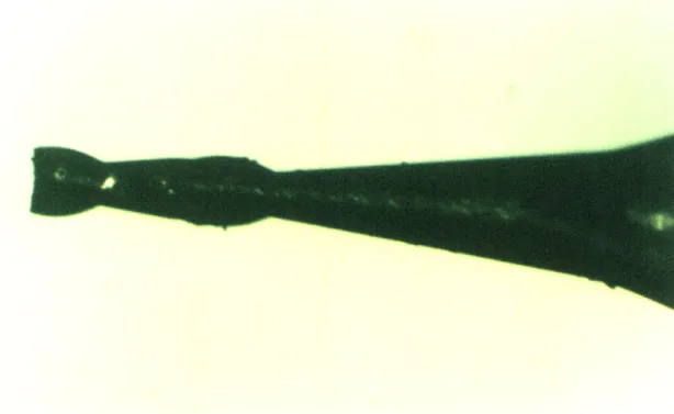
Figure 5.1: The 0.040" diameter endmill broken during machining the tool wear slot

sample. Most broken tools split at an angle rather than parallel to the plane of the tip. If the laser was measuring directly at the (now broken) tool tip, one might expect

the measurement value would come out significantly lower than the original tool

(51)

not measure at the broken point but instead evaluated the tool farther down towards its unbroken stem - perhaps the length sensing behavior conducted by the laser to find the tip fails when the tip is too small. The spindle rotates the tool while conducting the length and diameter measurements in order to perform a more uniform assessment. If

the broken tip of the tool has sheared at an angle, the revolutions of the tool would cause the tool tip-to-laser distance to alternate slightly with the rotation. It is not inconceivable that the machine might reposition the spindle and tool length-wise until this distance becomes constant, since in the case of an unbroken tool this would likely be an indication of correct tool tip positioning. Because the laser measurement process is entirely automated, there is no way to ensure how this measurement process is conducted or whether it is conducted properly on each run, and this is a downside.

On the other hand, in several later machining tests, tool breakage occurred in a way that was noticeable without graphical imagery. For example, the 0.040" endmill shown in Fig. 5.1 above broke violently enough that a cracking sound was heard. In addition, the snapped-off endmill tip became visibly embedded into the workpiece, and the spindle stopped rotating (though it should be mentioned that unexpected spindle starting and stopping were prevalent in these early machining tests, and such activity

may be unrelated to the tool breakage). However, other endmills - particularly those

0.010" in diameter and smaller - broke with no audio, visual, or machine-function cues, in which case it would have been advantageous if the laser tool was able to recognize such breaks. Of course, the earlier paragraph merely states that measurements of unknown-to-be-broken tools were found to be "reasonable enough" compared to expected value - a rather unspecific qualification related to the author's inexperience in working with tools of this scale.

5.1.2 Optical Microscope

The optical microscope was the most familiar of the four metrology methods and thus required little training time. However, the time that was not spent learning how to use the optical method was spent in specimen setup. Obtaining measurable images with the optical microscope proved somewhat more complicated and required a greater amount of time and care for tool setup than the previously discussed laser sensing

(52)

method. As discussed in Section 3.1, the experimental endmills were two-fluted, with the tip of each cutting edge located approximately 180 degrees apart. In order to obtain the correct measurement, the endmill needed to be oriented such that its tips were located at the upper-most and lower-most points on the tool (on the plane parallel with the slide) when imaged from the side, as demonstrated below in Fig. 5.2. In this

orientation, the vertical measurement from tip to tip measured the true diameter

-there was no perpendicular length component to account for, as would be the case otherwise. Fig. 5.3 demonstrates the potential for mis-measurements when a perpendicular length component exists.

Y Y

Z X

Figure 5.2: Correct positioning of an endmill on a microscope slide for true diameter

measurement. Note that the two cutting tips are oriented at the upper-most and lower-most points in the Y direction, so that a vertical measurement line drawn from tip to

tip measures the true diameter with no perpendicular Z-component [16].

Y

View direction

from

microscope

Figure 5.3: As the positioning of the two endmill tips rotates away from being vertically

aligned with the Y-axis, a perpendicular Z-axis component of the diameter is introduced that is not visible from the microscope view direction, potentially skewing

diameter measurements [17].

This mis-orientation occurred unintentionally in several cases and made re-imaging a necessity, such as in Fig. 5.4 below, which shows tool A, one of the 0.005" diameter endmills, misaligned and then correctly aligned.

(53)

Figure 5.4: The 0.005" diameter Tool A, misaligned (left) and correctly aligned (right).

On the medium- to large-sized endmills - those 0.020" in diameter and above -the tip features were visible to -the naked eye, allowing one to appropriately reposition the tool; however, smaller endmills often required several re-adjustments. Adjustments were somewhat tedious to perform, as removing the tool from the microscope to alter the orientation meant additional time was spent re-finding and refocusing the tool. Also, rotating the tool was done by hand. Given the small shaft size of the endmills, it was difficult to have much control over the angle of rotation - sometimes it was clear that only a small rotation was required, but even a small twist of the fingers would

realign the shaft too far.

Considering the diameter measurement was taken as the vertical distance from tip to tip as explained above, there was also the potential for mis-measurement if the tool was not aligned horizontally as shown in Fig. 5.5. The tool was only attached to the optical slide using fixturing gum, and while this gum prevented the endmill from rolling, it did not secure the tool solidly in place.

(54)

Figure 5.5: Top, a completely horizontal endmill, such that the vertical length

measurement from tip to tip correctly measured the diameter. Below, an unaligned endmill with an incorrectly measured diameter.

However, because this kind of alignment error was visible from the unmagnified side view, it was much more straightforward of a problem to fix. Adjustments could be made before the tool was located and focused through the microscope viewfinder. Thus, this was much less of an issue than the aforementioned rotation misalignment.

Optical microscopy also presented complications when preparing to measure due to its limited depth of field. Because only one depth could be clearly in focus at a given time, oftentimes the bulk of the tool edge would be unfocused as the contour followed a flute upwards or downwards in depth. On the other hand, the critical criterion for taking measurements was focusing just the very two tips. Provided the tool was in the correct alignment - both tips on a plane parallel to the microscope slide plane, and as

such at the same depth - the two tips would be in focus. Any blurriness outside of those

points was unfortunate from a graphical standpoint but was not problematic from a measurement standpoint. In fact, this was more of a problem with tools that were not perfectly rotationally aligned as described above, intrinsically providing another potential method of identifying misaligned tools. For example, in Fig. 5.6 are two images of a misaligned 0.015" D endmill, in which it is clear to see by adjusting the focus that the two cutting tips are not at the same depth of view.

(55)

Figure 5.6: On the left, the 0.015" diameter D endmill with its upper tip in focus and its

lower tip out of focus; on the right, the same tool and image, but with the focus shifted to the lower tip.

Also, the potential for experimenter bias should be noted here as well. For the milling machine laser sensing method, the experimenter had no control over the number output by the machine. Similarly, the digital and scanning electron microscopy methods were relatively unsusceptible to experimenter bias because the pixel coordinates of tool flute tips were collected and then converted into a diameter value. Without knowing the diameter value while collecting pixel coordinates, it was unlikely that the author tried to "fudge" results. However, in the case of the optical microscope software, the diameter measurement was presented on the screen with the point selector. Although not intentional, the author caught herself sometimes trying to pull the measurements more into sync with the nominal tool values. When noticed, these data were not used; however, it should be recognized that when presented the measurement value while in the process of measuring, the desire to collect "correct" results can sometimes be troublingly tempting.

5.1.3 Scanning Electron Microscope

Similar to the above analysis of the milling machine's laser sensing and optical microscopy, some of the first characteristics of the SEM method necessary to take into account are the setup-, training-, and measurement-times required for the process. There were several throughput-related drawbacks to using the SEM, especially when

(56)

considering its use for a student-run rapid prototyping project. The special holder for the tools, described in Section 3.2.4, was an additional pre-measurement task that required time. On the other hand, this step only needed to be completed once as the holder was reusable. Having the holder also sped up the imaging process considerably, since the machine did not need to be reloaded between tools; in addition, finding each

new tool was a simple matter of rotating the device a known amount - saving much of

the time and frustration that arose trying to find tools with both the optical and digital microscopes. Furthermore, an issue with both the abovementioned optical microscopy and the later-discussed digital microscopy was ensuring that the tool was aligned correctly - either lying perfectly horizontal in the case of the optical microscopy, or standing perfectly vertical in the case of the digital microscopy - so as to guarantee that diameter measurements were not impacted by introduction of perpendicular length components. Though the tools were aligned as best as possible by eye in the case of the optical and digital microscopy, it is assumed that the more precise holder required by

the SEM ensured a more precise vertical alignment. Naturally, this holder - with its

press-fit center stem removed - could be reused for tool alignment with the digital

microscope; it was not used for digital microscopy in this case simply because the SEM was used at a later date than the digital microscope.

While the initial inconvenience of specially machining a specimen holder for the SEM was ultimately beneficial, there were still several serious drawbacks to this method. While the author was trained to independently conduct the other metrology methods used in this project, using the SEM required a technical instructor to run the machine and supervise the process. This limited access was not only a scheduling problem, but prevented the opportunity for understanding the SEM process better. It is believed that the greater amount of time spent in direct use of each of the other three methods led to an increased sense of intuition about those methods. Had the time frame for this project been longer, it is likely training for the SEM could have been provided;

however, the likelihood that many users - for example, a set of students on an

undergraduate project - could be as easily trained on this device as the others seems much reduced.

(57)

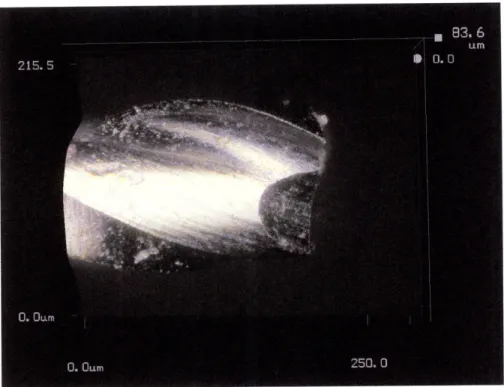
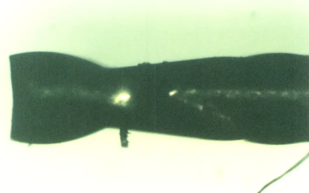
The SEM, like the optical microscope, could only focus at one distance, providing a limited depth of field. In some cases it was challenging to get the microscope to focus on the tool tip. Images of some tools, such as Fig. 5.7 of the 0.015" diameter tool D, clearly have the tool shaft more in focus than the tool tip, which made later image processing more difficult. Appropriate lighting also appeared to be a greater challenge with this method. The image of tool F, a 0.020" diameter endmill, is reproduced below in Fig. 5.8 to show how in some cases, the left half of the image was mostly obscured by darkness. Accurately pinpointing the flute tip of the darkened left side was difficult due to this lack of lighting.

Figure 5.7: Tool D, a 0.015" diameter endmill, has its shaft more in focus than its tip,