HAL Id: hal-02646891
https://hal.inrae.fr/hal-02646891
Submitted on 29 May 2020
HAL is a multi-disciplinary open access
archive for the deposit and dissemination of
sci-entific research documents, whether they are
pub-lished or not. The documents may come from
teaching and research institutions in France or
abroad, or from public or private research centers.
L’archive ouverte pluridisciplinaire HAL, est
destinée au dépôt et à la diffusion de documents
scientifiques de niveau recherche, publiés ou non,
émanant des établissements d’enseignement et de
recherche français ou étrangers, des laboratoires
publics ou privés.
Distributed under a Creative Commons Attribution - NoDerivatives| 4.0 International
density calculations: a comparison of approaches for
volume measurement
D. Maniatis, Laurent Saint-André, M. Temmerman, Y. Malhi, H. Beeckman
To cite this version:
D. Maniatis, Laurent Saint-André, M. Temmerman, Y. Malhi, H. Beeckman. The potential of using
xylarium wood samples for wood density calculations: a comparison of approaches for volume
mea-surement. iForest: Biogeosciences and Forestry, Italian Society of Silviculture and Forest Ecology,
2011, 4, pp.150 - 159. �10.3832/ifor0575-004�. �hal-02646891�
Standard Article - doi: 10.3832/ifor0575-004
©iForest – Biogeosciences and Forestry
Introduction
Tropical deforestation and degradation are estimated to have released on the order of 1 - 2 Pg C / yr (15 - 35 percent of annual fossil fuel emissions) during the 1990s (Houghton 2005). A key technical challenge for the suc cessful implementation of mechanisms that can help reduce emissions from deforestation and degradation is the reliable estimation of the aboveground biomass (AGB) in tropical forests. Reliable estimation of AGB depends on a number of sampling issues, including sampling of spatial variability, determination of forest structural allometry and determina tion of tree wood density, also known as wood specific gravity (WSG).
WSG is defined as the ratio of the oven-dry mass of a sample to the mass of a volume of water equal to the volume of the sample at a specific moisture content (ASTM Interna tional 2011) and is calculated by dividing the mass of a sample by its volume. Al though mass is easy to determine, the volume determination is a less straightfor
ward procedure. Moreover, sampling a suffi cient number of trees for WSG to represent the species and size distribution in highly di verse tropical forests is time consuming and costly. For tropical regions, published data on wood specific gravity are frequently limi ted to a number of commercial timber spe cies that only represent a fraction of the forest biomass.
On the other hand, there are collectively hundreds of thousand wood samples held in xylaria (botanical collection with wood samples from lignified plants (Beeckman 2008) around the world, spanning wide geo graphic areas including the tropics and many tens of thousands of species (Stern 1988).
Given the above, this paper focuses on WSG by: (1) exploring the possibility of ob taining the WSG of tropical tree species using xylaria samples; we examined the ac curacy and practicality of five different methodologies, two solid displacement me thods and three liquid displacement methods (of which two were specifically designed and
developed for the purposes of this paper); (2) measuring wood sample volume for the purpose of calculating WSG; and (3) provi ding a preliminary ecological assessment of WSG for 53 species in the Congo Basin in which we illustrate inter-individual variation in WSG, make a comparison of the WSG values of the species we measured to an ex isting wood density database, and examine genus-level WSG representativeness for spe cies-level WSG.
Background
There exists a great diversity of tropical woods with densities ranging from 0.1 (“light woods”) to 1.2 (“heavy woods”) g/cm3. WSG is considered as a crucial wood
property affecting the properties and value of both solid and fibrous wood products (Pliura et al. 2007). As a good predictor of mecha nical properties of wood, it is often viewed in relation to support against gravity, snow, wind and other environmental forces (Hacke et al. 2001).
Furthermore, WSG is an important factor for AGB estimates (Baker et al. 2004, Nogueira et al. 2005, Slik 2006). The most important predictors of ABG of a tree are its trunk diameter, wood specific gravity, total height and forest type (Chave et al. 2005). The most important source of error in AGB estimation is currently related to the choice of allometric model (Chave et al. 2005). However, ignoring variations in WSG can
(1) Environmental Change Institute, School of Geography and the Environment, Dyson Perrins Building, South Parks Road, OX1 3QY Oxford (UK); (2) CIRAD, UMR Eco & Sols, Ecologie Fonctionnelle, Biogéochimie des Sols & Agroécosystèmes, place Viala, F-34060 Montpellier (France); (3) INRA, UR BEF - Biogéochimie des Ecosystèmes Forestiers, F-54280, Champenoux (France); (4) Walloon Agricultural Research Centre (CRA-W), chaussée de Namur 146, B-5030 Gembloux (Belgium); (5) Laboratory for Wood Biology and Xylarium, Royal Museum for Central Africa, Leuvense Steenweg 13, B-3080 Tervuren (Belgium)
@
@
Danae Maniatis(danae.maniatis@gmail.com)
Received: Sep 15, 2010 - Accepted: May 16, 2011
Citation: Maniatis D, Saint André L,
Temmerman M, Malhi Y, Beeckman H, 2011. The potential of using xylarium wood samples for wood density calculations: a comparison of approaches for volume measurement. iForest 4: 150-159 [online 2011-08-11] URL:
http://www.sisef.it/iforest/ show.php? id=575
The potential of using xylarium wood
samples for wood density calculations: a
comparison of approaches for volume
measurement
Maniatis D
(1), Saint André L
(2-3), Temmerman M
(4), Malhi Y
(1),
Beeckman H
(5)Wood specific gravity (WSG) is an important biometric variable for above ground biomass calculations in tropical forests. Sampling a sufficient number of trees in remote tropical forests to represent the species and size distribution of a forest to generate information on WSG can be logistically challenging. Se veral thousands of wood samples exist in xylaria around the world that are ea sily accessible to researchers. We propose the use of wood samples held in xy laria as a valid and overlooked option. Due to the nature of xylarium samples, determining wood volume to calculate WSG presents several challenges. A de scription and assessment is provided of five different methods to measure wood sample volume: two solid displacement methods and three liquid dis placement methods (hydrostatic methods). Two methods were specifically de veloped for this paper: the use of laboratory parafilm to wrap the wood samples for the hydrostatic method and two glass microbeads devices for the solid displacement method. We find that the hydrostatic method with samples not wrapped in laboratory parafilm is the most accurate and preferred me thod. The two methods developed for this study give close agreement with the
preferred method (r2 > 0.95). We show that volume can be estimated accu
rately for xylarium samples with the proposed methods. Additionally, the WSG for 53 species was measured using the preferred method. Significant diffe rences exist between the WSG means of the measured species and the WSG means in an existing density database. Finally, for 4 genera in our dataset, the genus-level WSG average is representative of the species-level WSG average. Keywords: Wood specific gravity, Aboveground biomass, Dry xylarium samples, Tropical forests, Congo basin forest
result in mediocre overall prediction of the ABG biomass stand (Baker et al. 2004) greenhouse-gas emissions (Nogueira et al. 2005).
With regards to forest dynamics, WSG is related to the growth and mortality rates of a tree species (Muller-Landau 2004) and pro vides information on life-history strategies of tree species (King et al. 2005). Additionally, WSG is a strong indicator of ecological suc cession stages with the pioneer species ha ving greater variation and being less dense than climax species (Wiemann & William son 2002, Muller-Landau 2004). Several studies have shown that wood density is positively related to drought resistance in tropical trees (Hacke et al. 2001, Slik 2004) and shrubs (Hacke et al. 2000). Given the above, it is indeed unfortunate to find that the wood density of many tropical trees re mains unknown (Slik 2006).
As density is one of the most important parameters of wood quality, its measurement methods have been the subject of general publications on the physical properties of wood and moisture relations (cf. Simpson 1993, Simpson & TenWolde 1999) and spe cific measurement methods papers, such as: medical CAT-scan imaging for very small samples (Lindgren 1991); stereometric me thod (Rabier et al. 2006); mercury method (cf. Dutilleul et al. 1998); microdensitometer techniques (Cameron et al. 1959, Polge 1966, Mothe et al. 1998, Bergsten et al. 2001); basic density (dry weight / wet volu me) for freshly collected samples for conver sion to AGB (Fearnside 1997); vibrational spectroscopy such as near infrared reflec tance (NIR - Via et al. 2003, Via et al. 2005), Fourier Transform Infrared (FTIR) spectroscopic bands (Via et al. 2011) and Diffuse Reflectance Mid-Infrared Fourier transform (DRIFT-MIR - Nuopponen et al. 2006).
The above methods all have several ad vantages and disadvantages related to them. The main disadvantages related to some of the methods described above are: high cost; inability to take the xylarium samples out of the place they are stored (building); the fact that most samples do not have uniform or regular geometrical shapes; that the cutting of sub-samples is not allowed; and the phas ing out of mercury in many industries. What is clear is the need to develop feasible, prac tical, quick and cheap non-destructive meth ods to determine the volume of xylarium samples.
Material and methods
The wood sample collection
As a case study, we chose to focus on the major tropical forest region with perhaps the greatest deficit of ecological information: the Congo Basin Forest. The xylarium of the
museum for central Africa in Tervuren (Bel gium) holds the largest collection of wood samples for the Congo Basin Forest in the world (Beeckman 2007). Some samples have relatively precise descriptions of the trees (estimated height, large or small tree) and locations from where they were collected. There are also several samples per species, genus and family, making it possible to con duct a detailed study on the across- and within-taxon variability of WSG. The xyla rium also holds wood samples of what are now rare and protected species that could be difficult to collect today.
Particularities of using xylarium
samples
Due to the long-term mission of the xyla rium, samples are dry and have to remain in their original condition, i.e., the structural and chemical state of the sample must be preserved. Determining the WSG of such samples presents several difficulties. First, the format of the samples is not standard (e.g., irregular shapes, small planks, book shaped planks and circular pieces of wood). Second, it may not be allowed to cut pieces off the samples. Third, the samples may not be allowed to be covered in paraffin, wetted or treated with any chemical that may dama ge the sample, both in appearance and in any physical or molecular way. Last, the samples may perhaps not leave the designated area or be transported elsewhere for further studies.
Terminology
Of all the physical properties of wood, WSG was the first to be examined systema tically. An overview of the data from 18th
and beginning of 19th century has been given
by Chevandier & Wertheim (1848) in Koll mann (1951). We employ the terminology provided by the American Society for Tes ting and Materials (ASTM) specific gravity for wood can be defined as the ratio of the oven-dry mass of a sample to the mass of a volume of water equal to the volume of the sample at a specific moisture content (ASTM International 2011). Given that both the mass and, below the fibre saturation point, volume of wood vary with the amount of moisture contained in the wood, specific gravity as applied to wood is an indefinite quantity unless the conditions under which it is determined are clearly specified. The spe cific gravity of wood is based on the oven-dry mass, yet the volume may be that in the oven-dry, partially dry or green condition (ASTM International 2011).
Sample selection and preparation for
volume assessment
Two size categories of wood samples were selected: samples under 10 x 10 cm cross-sectional area and samples above 10 x 10 cm (hereafter referred to as “small” and “large”
samples, respectively). The samples are of ir regular shapes and sizes with varying de grees of surface smoothness. One hundred small samples were selected of 24 different species. For the large samples, 18 samples were selected of 15 different species.
To reach oven-dry mass, samples were dried in an oven for 48 hours: 2 hours at 60 °C, 4 hours at 80 °C and 42 hours at 103 °C to achieve constant weight. Temperature was increased gradually to minimise the risk of cracking the samples. Samples were weighed immediately after being taken out of the oven. The moisture content of the samples held in the xylarium before oven-drying (eqn. 1) was 8 percent. Samples under 2.1 g were weighed to the nearest 0.01 g while samples above 2.1 g were weighed to the nearest 0.1 g due to the limitations of the electronic balances used (eqn.1):
where mg is the mass of the wood sample as
held in the xylarium and mod is the oven dry
mass of the sample (attained after the oven drying and reaching constant mass). Volume measurements were done after the samples were oven dried and hence we measured an oven-dry WSG.
Sample selection for ecological assess
ment
The sample selection for a preliminary eco logical assessment focused on the regional scale of the Congo Basin Forest. Some 976 samples from 53 species were measured. Species were selected based on the following criteria: (1) each species needed to have a minimum of ten samples that could be mea sured; and (2) each species had to occur in more than one region of the Congo Basin forest.
A comparison was made between the spe cies means for the measured species and the means of the same species found in the Global Wood Density Database (GWDD - Zanne et al. 2009) using a two-sample t-test assuming unequal variances at a five percent significance level. In order to evaluate whether or not genus-level WSG averages were representative of species-level WSG averages, a nested analysis of variance (ANOVA) was used.
Liquid displacement methods
These are methods based on Archimedes’ principle: the volume of a sample is esti mated by the mass of the volume that is dis placed while the sample is submerged in li quid. The method used for this study is known as the hydrostatic method. In this method, the mass of the liquid which is dis placed by the sample (oven-dry) is deter mined. A beaker is filled with water and
MC=(mg−mod)
mod
Measuring the volume of wood samples
placed on a digital balance. The balance is then re-zeroed. The sample is attached to an adjustable screw clamp (of which the volume is known and corrected for when submerged in the water), which is in turn attached to a vertically moving arm of a stand. The mea sured weight of displaced water equals the sample’s volume (since water has a density of 1). The electronic balance was re-zeroed after every measurement. Three repetitions were made for each sample with the hydro static method. Three variations of the hydro static method were tested, using the same principle as described above and the same samples:
1. Samples wrapped in laboratory parafilm. The samples were weighed before coating and after coating them in laboratory para film. The difference in weight was sub tracted from the volume of the sample. The disadvantage with laboratory parafilm wrapping is that it may trap air. Wrapping the wood samples in laboratory parafilm was developed specifically for the pur poses of this paper. We used laboratory parafilm “M” which is water repellent and self-adhesive.
2. Samples not wrapped in laboratory para
film. The volume of the sample was taken,
the sample was dried off and the following repetition was made. Samples were not re-weighed after each measurement to ac count for increase in weight.
3. Samples not wrapped in laboratory para
film, with re-weighing the samples after each measurement in order to take account
of increase in weight due to water absorp tion. The sample was weighed, the volume was of the sample was taken, the sample dried off, its weight taken, the difference in weight added to the volume of the sample (accounting for absorption) and the follo wing repetition made.
Solid displacement method
These methods are based on the principle that solid materials are used to measure the volume of a given sample. Two solid dis placement methods were tested:
1. Sand using a vibrating bed for compac
tion. For this method calibrated white sand
was used. Sand was poured into a glass beaker until reaching a required volume (e.g., 100 ml). The beaker containing the sand was placed on a vibrating bed for 10 seconds to ensure compaction of the sand particles at a predefined volume (e.g., 100 ml). In a second glass beaker recipient, some of the sand was poured in to cover the bottom of the recipient and subse quently the sample was placed on the sand. The rest of the sand was poured on top of the sample until the sand containing the sample reached the same initial volume (100 ml) once again followed by compac ting the sand on the vibrating bed. The re
maining sand (again compacted) represents the volume of the sample. Two repetitions were made for each sample. A third mea surement was taken if the difference between the two volume measurements was above 5 percent.
2. Glass microbeads using height drop for
compaction. This machine was designed
specifically for this study (Fig. 1). The concept of the machine is a semi-closed system of two glass recipients connected by a graduated cylinder (each 2 ml gradua tion) held in a wooden structure. Two ma chines were built, one for small samples and one for larger samples. For the small samples, the volume of the graduated cy linder is 100 ml and approximately 95 cm in vertical height. For the large samples, the graduated cylinder is 1000 ml and the vertical height approximately 110 cm. The method works like an hourglass. There is a constant amount of glass microbeads in the glass recipients (of 0.5 micrometers), the volume of which is read off the graduated cylinder (e.g., 20 ml). The system is ro tated on its own axis and the glass mi cro-beads run into the second glass reci pient. The sample is placed in the first glass recipient that can be opened. Once the sample is placed in the container, the system is turned around on its axis once more. The volume is once again read (e.g., 50 ml) and the difference in volume is the volume of the sample (e.g., in this example the volume equals to 30 ml). Two repeti tions were made for each small sample. If the difference was greater than 5 percent, a third repetition was made. Three repeti tions were made for the large samples. To test the accuracy of the two machines
with known volume samples, the Walloon Agricultural Research Centre conducted the volume measurements on 56 different samples. Different defined shapes with smooth surfaces and known volumes were produced and measured using in the devices. For the smaller device, 10 cubic shaped samples (8.1 to 263 cm3), 10 cylindrical
shaped samples (3.4 to 279 cm3) and 10 par
allelepiped shaped samples (16.7 to 184 cm3) were processed in 5 replications. For
the larger device, the 8 cubic shaped samples (126 to 700 cm3), 9 cylindrical shaped
samples (30 to 1127 cm3) and 10 paral
lelepiped shaped samples (91.6 to 310 cm3)
were processed in 5 replications.
To evaluate the influence of each tested method on the wood sample density results, individual and global mean values, we calcu lated mean WSG and two measures of dis persion, the standard deviation and coeffi cient of variation of the WSG values (Wie mann & Williamson 2002). To compare the mean values of WSG obtained by the diffe rent methods, ANOVA were conducted at a significance level of 5 percent. A one-way ANOVA procedure was used for pair-wise multiple comparisons. The agreements between the chosen “preferred” method and other methods were evaluated using the coefficient of determination (r2) and the
F-statistical test for bias, slope = 1 and inter cept = 0 using SAS software (Mayer & But ler 1993, Leroy et al. 2007).
Results and discussion
Tab. 1 shows the mean densities (g/cm3)
and density ranges (g/cm3) for the measured
wood samples. The sand method was only used for the 100 small samples. It appears to
overestimate mean density and the standard deviation is highest. On the other hand, the glass microbeads method appears to under estimate WSG. Besides the case for the 18 large samples, this underestimation is similar to the underestimation when using labora tory parafilm. With the glass microbeads, it might be that the compaction of the beads is insufficient, giving a higher volume for the samples. For the wood samples wrapped in parafilm the increased volume is most likely due to the trapping of air between the sample and the parafilm. The mean densities of the hydrostatic method correcting for absorption and the mean densities of the plain hydro
static method are very similar. The patterns described can be observed clearly when looking at a randomly chosen samples (Fig. 2).
Large standard deviations for the sand and glass microbeads method are observed (Fig. 2: S4, S5, S7, S9, S10, S13, S14, S15 and S16). Assuming that the samples did not fall into the same position within the glass cylin ders at each repetition, perhaps the sand particles and glass microbeads could not compact around the sample in the same man ner, explaining the larger variation.
We performed an ANOVA on three sets of data: (1) 100 small samples; (2) the 18 large
samples; and (3) the small and large samples put together (see below).
1. Small samples: the method has a signifi cant effect on the estimation of density (p < 0.01). The Levene statistics test rejects the null hypothesis that the group varian ces are equal (p >0.05). Using Tamhanes’ test which does not assume equal varian ces, for the small samples, we find that there is a significant difference between the glass microbeads method and the sand method (p < 0.01), the sand method and the hydrostatic parafilm method (p < 0.01) and between the sand method and the hy drostatic method (p < 0.05);
Fig. 2 - Wood sample density for 10 small samples and 6 large samples estimated by five different methods. The y-axis shows the wood spe
cific gravity of a sample depending on the method used. Each column on the x-axis represents the WSG values for one sample. The sand method is only used for the small samples. Error bars show the standard deviation. S1 stands for sample 1 and so on.
Tab. 1 - Summary table of mean densities ± SE (g/cm3) and density ranges (g/cm3).
Method 100 small samples 18 large samples Combination of samples (118) Mean
density Densityrange densityMean Densityrange densityMean Densityrange
Sand
(solid displacement) 0.79 ± 0.24 0.22 ÷ 1.62 - - -
-Glass micro-beads
(solid displacement) 0.65 ± 0.18 0.16 ÷ 0.98 0.62 ± 0.22 0.24 ÷ 1.12 0.65 ± 0.18 0.16 ÷ 1.12 Wrapped in laboratory parafilm
(hydrostatic) 0.65 ± 0.17 0.17 ÷ 0.97 0.64 ± 0.20 0.29 ÷ 1.04 0.65 ± 0.17 0.17 ÷ 1.04 Not wrapped in laboratory parafilm and not correcting
for absorption (hydrostatic) 0.70 ± 0.18 0.19 ÷ 1.04 0.69 ± 0.21 0.30 ÷ 1.10 0.70 ± 0.19 0.19 ÷ 1.10 Not wrapped in laboratory parafilm but accounting for
Measuring the volume of wood samples
2. Large samples: the choice of method has no significant effect on the mean density (p > 0.05). The Levene statistics test rejects the null hypothesis that the group vari ances are equal (p > 0.05). Using Tam hanes’ statistic, we find that there is no si gnificant difference between the groups on mean density. Indeed, it appears that the sand method used on the small samples was the most problematic;
3. Combined: we find that choice of method has a slight but significant effect on the mean density (p < 0.02). The Levene stati stics test rejects the null hypothesis that the group variances are equal (p > 0.05). Using Tamhanes’ statistic, we find that there is no significant difference between the groups on mean density.
Regarding the hydrostatic method for samples not wrapped in parafilm but
re-weighing after each measurement (correcting for absorption), there is an increase in volu me for the samples when absorption is taken into account. There is an average volume in crease of 0.61 percent for small samples and 0.29 percent for large samples. This has an impact of 0.61 percent on the mean density of the small samples and 0.29 percent for the large samples, affecting the mean density by the same amounts. This percentage can be regarded as negligible meaning that either hydrostatic method with samples not wrap ped in parafilm could be a “preferred” choice of method. Not wrapping the samples in parafilm but correcting for absorption was chosen as the “preferred” method based on its precision and comprehensive approach for this study. However, this choice should be evaluated for each study and could, for example, be ranked on an assessment of an
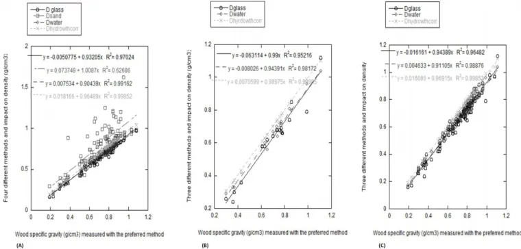
allowable error for the WSG measurement. All subsequent regression analyses use the “preferred” method against which the other four methods are tested (Fig. 3 and Tab. 2). The relationships between the preferred me thod and other methods were satisfactory for all methods excluding the sand method. For the small samples, the large samples and the small and large samples combined, the coef ficient of determination for: (a) the hydro static method (without parafilm or correction for absorption), (b) the hydrostatic method with parafilm, and (c) the glass microbeads method is highly significant (r2 > 0.95 in all
cases). Hence, any of these three other me thods are valid depending on the limitations of the samples to be worked with. However, the simultaneous F-test for bias, slope = 1 and intercept = 0 was significant for all methods and small, large or combined
Fig. 3 - Regression analyses comparing the “preferred method” (hydrostatic method without parafilm wrapping but with correction to take
account of water absorption) to the other different tested methods: (A) for 100 measured small samples, (B) for 18 measured large samples and (C) for all measured samples.
Tab. 2 - Statistical summary of linear regression (F-statistic) of the preferred method against the other methods. Slope H0 = 1, intercept H0 =
0; (*): p < 0.05; (**): p < 0.01; (***): p < 0.001.
Preferred method Sand Glass micro-beads Wrapped in laboratory parafilm parafilm and not correctingNot wrapped in laboratory for absorption Linear regression 100 small samples 100 small samples 18 large samples combined 100 small samples 18 large samples combined 100 small samples 18 large samples combined
Adjusted R2 0.63 0.97 0.95 0.96 0.99 0.98 0.99 1 1 1
Slope 0.62***± 0.05 1.04*± 0.02 0.96± 0.05 1.02± 0.02 ± 0.011.1*** 1.04± 0.04 1.09***± 0.01 1.03*** ± 0.0 1.0± 0.0 1.03*** ± 0.0 Intercept 0.22***± 0.04 0.03*± 0.01 0.1*± 0.04 0.04***± 0.01 ± 0.01-0.00 0.02± 0.02 0.0 ± 0.01 -0.02***± 0.0 -0.0± 0.0 -0.01***± 0.0 Bias 55.35*** 140.46*** 19.63*** 144.82*** 700.52*** 21.35*** 525.06*** 100.48*** 2.2 77.69*** % under or overestimation 38% -4% 4% -2% -10% -4% -9% -3% (none) -3%
samples (p < 0.001) but one: the 18 large samples not wrapped in laboratory parafilm. The slope was significantly different from 1 for sand - 100 small samples; glass mi crobeads - 100 small samples; not wrapped in laboratory parafilm - 100 small samples and combined. The intercept was signifi cantly different from 0 for sand; all three ca tegories of samples for glass microbeads; not wrapped in laboratory parafilm - 100 small samples and combined.
The analysis of the coefficient of variation shows that the shape of the sample did not influence the precision of the method (Fig. 4). On the other hand, it is clear that the coefficient of variation is higher for lower volumes. Moreover, the variation is higher for the larger device, compared to the small one. In order to improve the precision of the method it is advisable (Tab. 3) to avoid the use of small samples. The relative accuracy of the method improved from 2.30 percent (all tested samples) to 1.29 percent (sample volume > 20 cm3) for the small device and
from 3.60 percent (all tested samples) to
2.74 percent (sample volume > 100 cm3) for
the larger device.
Preliminary ecological application
We provide a preliminary ecological as sessment of the data collected. The WSG of the samples was measured using the pre ferred method. Tab. 4 provides a summary of the WSG values for each of the 53 species and compares the measured values to the values found in the GWDD (Zanne et al. 2009). For the species where a comparison of the averages could be made between the measured means and the means derived from the GWDD, there exists a significant diffe rence between the means (p < 0.05 - indi cated in Tab. 4 with an asterisk).Where two or more species in a genus are present in our dataset, genus-level WSG ave rages were calculated (Tab. 5). Although this dataset is not as extensive, our data indicates that the four genus-level WSG averages can be considered as representative of their spe cies-level WSG averages (the genus effect is significant at p < 0.01) for Central Africa,
similar to what Baker et al. (2004) observe in Amazonia.
We observe a considerable variation in WSG within many species (Fig. 5). How ever, it is important to highlight that al though some xylarium samples include in formation on tree location (with variable ac curacy), the position in the tree from which the sample was drawn is not available. As it is well known that wood density can vary substantially within, as well as between trees (Zobel & van Buijtenen 1989), this might partially explain the large variations in some species. Furthermore, marked variations in WSG may be observed for a tree species which are attributable to differences in site quality and/or forest types (Patiño et al. 2009) and site specific differences have been observed comparing the same species gro wing in different site conditions or forest types (e.g., Nogueira et al. 2005, Nogueira et al. 2007).
Conclusion
The purpose of this paper was to: (1) high light the potential use of xylarium samples to measure WSG; (2) provide an assessment on determining wood sample volume to calcu late WSG from dry xylarium samples that have to be preserved in their original state; and (3) contribute and compare the WSG values of the 53 measured species in the Congo Basin Forest to existing databases and present a preliminary ecological assess ment of the interindividual variation in WSG and the representativeness of genus-level averages compared to species-level averages.
Tab. 3 - Precision of the different sample sizes and glass microbeads devices used.
Method Avg. STD Avg. CV (%) for N = 5 (%)Accuracy dr
Small device/All samples 0.78 1.85 2.30 Small device / sample volume > 20
cm3 0.84 1.04 1.29
Large device / All samples 6.00 2.90 3.60 Large device / Sample volume >
100 cm3 6.13 2.21 2.74
Measuring the volume of wood samples Tab. 4 - WSG of the measured samples per species compared to the WSG values in the GWDD. WSG values from the GWDD were taken
for species occurring in Africa, as the measured species all originate from Central Africa. An asterisk (*) next to a species name indicates a significant difference (p < 0.05) between the mean of the measured values and the mean of that species in the GWDD.
Species No. Samples measured Average WSG ± STD (g/cm3) Range WSG(g/cm3)
No. values given in GWDD WSG value GWDD ± STD (g/cm3) WSG value GWDD range (g/cm3) Albizia adianthifolia 15 0.56 ± 0.13 0.38 - 0.86 7 0.51 ± 0.06 0.45 - 0.65 Albizia gummifera 19 0.57 ± 0.08 0.43 - 0.71 7 0.53 ± 0.06 0.47 - 0.65 Alstonia congensis 12 0.35 ± 0.09 0.27 - 0.62 8 0.33 ± 0.03 0.29 - 0.39 Autranella congolensis* 20 0.88 ± 0.09 0.56 - 1.00 9 0.75 ± 0.11 0.55 - 0.87 Canarium schweinfurthii 15 0.44 ± 0.10 0.22 - 0.57 16 0.41 ± 0.06 0.30 - 0.55 Ceiba pentandra 10 0.30 ± 0.06 0.18 - 0.38 14 0.28 ± 0.03 0.22 - 0.35 Chlorophora excelsa (Milicia excelsa) 48 0.57 ± 0.07 0.37 - 0.73 24 0.58 ± 0.06 0.44 - 0.67 Dacryodes edulis 11 0.62 ± 0.17 0.50 - 0.94 3 0.52 ± 0.02 0.50 - 0.53 Diospyros crassiflora* 6 1.05 ± 0.08 0.91 - 1.14 5 0.86 ± 0.09 0.77 - 0.99 Entandrophragma angolense* 21 0.57 ± 0.09 0.44 - 0.80 15 0.48 ± 0.04 0.44 - 0.59 Entandrophragma candollei 23 0.58 ± 0.10 0.33 - 0.75 10 0.57 ± 0.07 0.42 - 0.67 Entandrophragma cylindricum 24 0.60 ± 0.05 0.50 - 0.70 16 0.57 ± 0.04 0.50 - 0.63 Entandrophragma utile* 17 0.59 ± 0.06 0.50 - 0.75 18 0.54 ± 0.04 0.44 - 0.58 Gilbertiodendron dewevrei* 41 0.78 ± 0.06 0.64 - 0.87 4 0.71 ± 0.02 0.68 - 0.73 Gossweilerodendron balsamiferum* (Prioria balsamifera) 32 0.48 ± 0.08 0.33 - 0.71 9 0.41 ± 0.04 0.31 - 0.45 Guarea cedrata* 17 0.63 ± 0.06 0.55 - 0.78 15 0.51 ± 0.03 0.46 - 0.59 Guarea laurentii* 15 0.63 ± 0.05 0.55 - 0.72 3 0.56 ± 0.02 0.54 - 0.59 Hallea stipulosa* 21 0.56 ± 0.10 0.44 - 0.77 7 0.48 ± 0.03 0.45 - 0.53 Khaya anthotheca* 19 0.54 ± 0.07 0.41 - 0.67 11 0.49 ± 0.04 0.44 - 0.55 Klainedoxa gabonensis 17 0.87 ± 0.16 0.47 - 1.05 12 0.93 ± 0.10 0.78 - 1.15 Lovoa trichilioides* 18 0.58 ± 0.08 0.47 - 0.77 19 0.45 ± 0.04 0.39 - 0.53 Maesopsis eminii 8 0.44 ± 0.16 0.34 - 0.82 3 0.40 ± 0.02 0.37 - 0.41 Mammea africana* 21 0.70 ± 0.09 0.44 - 0.85 16 0.63 ± 0.04 0.57 - 0.71 Millettia laurentii 19 0.79 ± 0.06 0.67 - 0.90 8 0.76 ± 0.05 0.72 - 0.88 Morinda lucida 14 0.60 ± 0.06 0.53 - 0.74 - - -Musanga cecropioides 27 0.21 ± 0.09 0.13 - 0.46 12 0.24 ± 0.07 0.16 - 0.39 Myrianthus arboreus 7 0.55 ± 0.05 0.47 - 0.60 - - -Nauclea diderrichii* 19 0.71 ± 0.04 0.63 - 0.80 22 0.68 ± 0.04 0.59 - 0.78 Ongokea klaineana ( Ongokea gore) 29 0.76 ± 0.08 0.56 - 0.88 10 0.75 ± 0.04 0.69 - 0.83 Panda oleosa 10 0.67 ± 0.07 0.57 - 0.81 1 0.57 -Pentaclethra eetveldeana 15 0.73 ± 0.13 0.55 - 0.99 1 0.66 -Pentaclethra macrophylla 15 0.80 ± 0.18 0.54 - 1.03 9 0.84 ± 0.07 0.73 - 0.94 Pericopsis elata* 14 0.70 ± 0.08 0.60 - 0.87 12 0.64 ± 0.04 0.57 - 0.71 Petersianthus macrocarpus* 45 0.73 ± 0.09 0.46 - 0.90 10 0.68 ± 0.06 0.57 - 0.77 Polyalthia suaveolens 19 0.72 ± 0.05 0.61 - 0.82 1 0.70 -Prioria oxyphylla (Oxystigma oxyphyllum) 16 0.60 ± 0.06 0.50 - 0.80 4 0.57 ± 0.05 0.53 - 0.65 Pterocarpus soyauxii* 20 0.72 ± 0.08 0.52 - 0.86 14 0.66 ± 0.07 0.57 - 0.81 Pterocarpus tinctorius 14 0.65 ± 0.20 0.31 - 0.90 - - -Ricinodendron heudelotii* 14 0.26 ± 0.08 0.15 - 0.47 5 0.21 ± 0.02 0.19 - 0.23 Scorodophloeus zenkeri 16 0.76 ± 0.10 0.45 - 0.87 4 0.72 ± 0.09 0.60 - 0.81 Staudtia kamerunensis (Staudtia stipitata) 51 0.80 ± 0.07 0.61 - 0.94 17 0.80 ± 0.07 0.65 - 0.92 Strombosia grandifolia* 16 0.75 ± 0.05 0.67 - 0.83 6 0.82 ± 0.06 0.75 - 0.91 Strombosiopsis tetrandra 18 0.73 ± 0.08 0.51 - 0.89 1 0.66 -Symphonia globulifera* 20 0.68 ± 0.09 0.51 - 0.84 8 0.59 ± 0.06 0.46 - 0.65 Syzygium guineense* 6 0.71 ± 0.08 0.64 - 0.87 3 0.61 ± 0.04 0.58 - 0.65 Terminalia superba* 15 0.54 ± 0.11 0.34 - 0.83 57 0.46 ± 0.06 0.32 - 0.62 Tetrorchidium didymostemon 8 0.44 ± 0.07 0.32 - 0.55 1 0.44 -Treculia Africana 6 0.67 ± 0.07 0.59 - 0.78 - - -Trema orientalis (Trema guineensis) 20 0.51 ± 0.15 0.30 - 0.82 1 0.42 -Uapaca guineensis* 9 0.71 ± 0.07 0.62 - 0.84 7 0.61 ± 0.07 0.54 - 0.71 Vitex madiensis 6 0.55 ± 0.09 0.47 - 0.72 - - -Xylopia aethiopica 21 0.59 ± 0.10 0.44 - 0.77 2 0.44 ± 0.11 0.36 - 0.52 Zanthoxylum gilletii (Fagara macrophylla) 16 0.71 ± 0.13 0.49 - 0.96 11 0.69 ± 0.14 0.47 - 0.87
To estimate wood volume of xylarium samples to calculate WSG, we generallyre commend the hydrostatic approach of not wrapping samples in laboratory parafilm. As the impact on WSG of correcting for absorp tion is negligible, this is not necessary. Com paring the hydrostatic method for samples not wrapped in parafilm but correcting for absorption to the other two hydrostatic me thods (i.e., either with parafilm, or without parafilm but without correction for absorp tion) and the glass microbeads method resul ted in a high r2 value (> 0.95). This suggests
that any of these other three methods are va lid depending on the limitations of the samples one would be working with and the objectives of the study. Hence, we have
shown the validity of using laboratory para film to wrap samples for the hydrostatic method and the glass microbeads construc tion. When samples cannot be immersed in water in any circumstances, the glass mi crobeads construction offers a reliable alter native. When possible, using sterile water in stead of tap water may further increase the precision of the hydrostatic methods.
This study also illustrates the contribution that the measurement of xylarium samples can make to existing global wood density databases. This contribution consists both in adding species that are currently not present in the database, but also helping to improve the current database estimates by increasing the number of measurements. Although the
data presented is by no means extensive, it does illustrate the intervariability in WSG within and between species and suggest that genus-level WSG averages may indeed be representative of species-level WSG ave rages in the Congo Basin.
In a broader context, we have illustrated that, although working with xylarium sam ples brings several methodological chal lenges, these can be overcome to enable the use of xylarium samples to calculate WSG. In this way, xylaria hold a great amount of untapped information on taxonomic, spatial and potentially temporal variation in wood specific gravity that could be useful for eco logists, especially for providing more robust estimates of aboveground biomass and un derstanding of forest dynamics.
Acknowledgments
We thank Pol Dricot for constructing the glass microbeads machines and the handling of samples for testing the accuracy of the glass microbeads method. We also thank Nicolas Barbier and three reviewers for hel ping us to improve the manuscript.
Fig. 5 - Boxplot showing the inter-individual variation in WSG for the 53 measured species. The boxplot also shows the notches for each
species: two medians are significantly different at the 5 percent significance level if their intervals (interval endpoints are the extremes of the notches) do not overlap. The figure also shows the whiskers of which the length w is set at 1.5. Points are drawn as outliers (crosses) if they are larger than q3 + w(q3 - q1) or smaller than q1 - w(q3 - q1), where q1 and q3 are the 25th and 75th percentiles, respectively. The whisker plot
ted on the figure extends to the adjacent value, which is the most extreme data value that is not an outlier.
Tab. 5 - Genus-level averages for four genera of the dataset.
Genus samplesNo. Average WSG ± STD (g/cm3)
Albizia 34 0.57 ± 0.11
Entandrophragma 68 0.58 ± 0.08
Pentaclethra 30 0.77 ± 0.16
Measuring the volume of wood samples
References
ASTM International (2011). ASTM D2395 - 07ae1 Standard test methods for specific gravity of wood and wood-based materials. Web page. [online] URL: http://www.astm.org/Standards/ D2395.htm
Baker TR, Philips OL, Malhi Y, Almeida S, Ar royo L, Di Fiore A, Erwin T, Killeen TJ, Susan G, Laurance SG, Laurance WF, Lewis SL, Lloyd J, Monteagudo A, Neill DA, Patiño S, Pitman NCA, Silva JNM, Vásquez Martínez R (2004). Variation in wood density determines spatial pat terns in Amazonian forest plots. Global Change Biology 10: 1-18. - doi: 10.1111/j.1365-2486. 2004.00751.x
Beeckman H (2008). A xylarium for the sustai nable management of biodiversity: the wood col lection of the royal museum for central Africa, Tervuren, Belgium. Le bulletin de l’APAD no. 26, Gestion des Ressources Naturelles. Participa tions et médiations. [online] URL: http://apad.re vues.org/document3613.html
Beeckman H (2007). Wood. Collections of the Royal Museum for central Africa. Collections of the Royal Museum for Central Africa, Belgium, pp.112. [ISBN: 978-90-74752-17-6]
Bergsten U, Lindeberg J, Rindby A, Evans R (2001). Batch measurements of wood density on intact or prepared drill cores using x-ray mi crodensitometry. Wood Science and Technology 35: 435-452. - doi: 10.1007/s002260100106
Cameron JF, Berry PF, Phillips EWJ (1959). The determination of wood density using beta rays. Holzforschung 13: 78-84. - doi: 10.1515/hfsg. 1959.13.3.78
Chave J, Andalo C, Brown S, Cairns MA, Cham bers JQ, Eamus D, Fölster H, Fromard F, Higu chi N, Kira T, Lescure JP, Nelson BW, Ogawa H, Puig H, Riéra B, Yamakura T (2005). Tree al lometry and improved estimation of carbon stocks and balance in tropical forests. Oecologia 145 (1): 87-99. - doi: 10.1007/s00442-005-0100-x
Dutilleul P, Herman M, Avella-Shawn T (1998). Growth rate effects among ring width, wood density, and mean tracheid length in Norway spruce (Picea abies). Canadian Journal of Forest Research 28: 56-68. - doi: 10.1139/x97-189
Fearnside PM (1997). Wood density for estima ting forest biomass in the Brazilian Amazon. Forest Ecology and Management 90: 59-87. - doi: 10.1016/S0378-1127(96)03840-6
Hacke UG, Sperry JS, Pittermann J (2000). Drought experience and cavitation resistance in six shrubs from the Great Basin, Utah. Basic and Applied Ecology 1 (1): 31-41. - doi: 10.1078/ 1439-1791-00006
Hacke UG, Sperry JS, Pockman WT, Davis SD, McCulloh KA (2001). Trends in wood density and structure are linked to prevention of xylem implosion by negative pressure. Oecologia 126: 457-461. - doi: 10.1007/s004420100628
Houghton R (2005). Tropical deforestation as a source of greenhouse-gas emissions. In: “Tropi cal deforestation and climate change” (Moutinho P, Schwartzmann S eds). IPAM, Instituto de
Pesquisa Ambiental da Amazônia, Belém, Pará, Brazil - Environmental Defense, Washington DC, USA.
King DA, Davies SJ, Nur Supardi MN, Tan S (2005). Tree growth is related to light intercep tion and wood density in two mixed dipterocarp forests of Malaysia. Functional Ecology 19: 445-453. - doi: 10.1111/j.1365-2435.2005.00982.x
Kollmann F (1951). Technologie des holzes und der holzwerkstoffe. Zweite auflage. I. Band. Springer-Verlag, Berlin - Göttingen, Heidelberg - Bergmann JF, München, pp. 1050.
Leroy C, Saint-André L, Auclair D (2007). Prac tical methods for non-destructive measurement of tree leaf area. Agroforestry Systems 71: 99-108. - doi: 10.1007/s10457-007-9077-2
Lindgren LO (1991). The accuracy of medical CAT-scan images for non-destructive density measurements in small volume elements within solid wood. Wood Science and Technology 25 (6): 425-432. - doi: 10.1007/BF00225235
Mayer DG, Butler DG (1993). Statistical valida tion. Ecological Modelling 68 (1-2): 21-32. - doi:
10.1016/0304-3800(93)90105-2
Mothe F, Duchanois G, Zannier B, Leban JM (1998). Analyse microdensitométrique appliquée au bois: méthode de traitement des données uti lisée à l’INRA-ERQB (programme CERD). An nales des Sciences Forestières 55 (3): 301-313. - doi: 10.1051/forest:19980303
Muller-Landau HC (2004). Interspecific and inter-site variation in wood specific gravity of tropical trees. Biotropica 36 (1): 20-32. - doi: 10.1111/ j.1744-7429.2004.tb00292.x
Nogueira EM, Nelson BW, Fearnside PM (2005). Wood density in dense forest in central Amazo nia, Brazil. Forest Ecology and Management 208: 261-286. - doi: 10.1016/j.foreco.2004.12. 007
Nogueira EM, Fearnside PM, Nelson BW, França MB (2007). Wood density in Brazil’s “arc of de forestation”: implications for biomass and flux of carbon from land-use change in Amazonia, Brazil. Forest Ecology and Management 248: 119-135. - doi: 10.1016/j.foreco.2007.04.047
Nuopponen MH, Birch GM, Sykes RJ, Lee SJ, Stewart D (2006). Estimation of wood density and chemical composition by means of Diffuse Reflectance Mid-Infrared Fourier Transform (DRFT-MIR) spectroscopy. Journal of Agricul tural and Food Chemistry 54: 34-40. - doi:
10.1021/jf051066m
Patiño S, Lloyd J, Paiva R, Baker TR, Quesada CA, Mercado LM, Schmerler J, Schwarz M, Santos AJ, Aguilar A, Czimczik CI, Gallo J, Hor na V, Hoyos EJ, Jimenez EM, Palomino W, Pea cock J, Peña-Cruz A, Sarmiento C, Sota A, Tur riago JD, Villanueva B, Vitzthum P, Alvarez E, Arroyo L, Baraloto C, Bonal D, Chave J, Costa AC, Herrera R, Higuchi N, Killeen T, Leal E, Luizão F, Meir P, Monteagudo A, Neil D, Núñez-Vargas P, Peñuela MC, Pitman N, Priante Filho N, Prieto A, Panfil SN, Rudas A, Salomão R, Silva N, Silveira M, Soares dealmeida S, Tor res-Lezama A, Vásquez-Martínez R, Vieira I, Malhi Y, Phillips OL (2009). Branch xylem
density variations across the Amazon Basin. Biogeosciences 6 (4): 545-568. - doi: 10.5194/ bg-6-545-2009
Pliura A, Zhang SY, MacKay J, Bousquet J (2007). Genotypic variation in wood density and growth traits of poplar hybrids at four clonal tri als. Forest Ecology and Management 238: 92-106. - doi: 10.1016/j.foreco.2006.09.082
Polge H (1966). Établissement des courbes de variation de la densité du bois par exploration densitométrique de radiographies d’échantillons prélevés à la tarière sur des arbres vivants - Ap plications dans les domaines technologique et physiologique. Ph.D. Dissertation, Université de Nancy-1, Champenoux, France, pp. 215. Rabier F, Temmerman M, Böhm T, Hartmann H,
Daugberg Jensen P, Rathbauer J, Carrasco J, Fernández M (2006). Particle density determina tion of pellets and briquettes. Biomass and Bioenergy 30: 954-963. - doi: 10.1016/j.biom bioe.2006.06.006
Simpson W, TenWolde A (1999). Physical pro perties and moisture relations of wood. In: “Forest products laboratory. Wood handbook - wood as an engineering material. Gen. Tech. Rep. FPL-GTR-113, Forest Products Laboratory, USDA Forest Service, Madison, WI, USA, pp. 463.
Simpson WT (1993). Specific gravity, moisture content, and density relationships for wood. Gen. Tech. Rep. FPL-GTR-76, Forest Products Labo ratory, USDA Forest Service, Madison, WI, USA, pp. 13.
Slik JWF (2004). El Nino droughts and their ef fects on tree species composition and diversity in tropical rain forests. Oecologia 141: 114-120. - doi: 10.1007/s00442-004-1635-y
Slik JW (2006). Estimating species-specific wood density from the genus average in Indonesian trees. Journal of Tropical Ecology 22 (04): 481. - doi: 10.1017/S0266467406003324
Stern WL (1988). Index xylariorum. Institutional wood collections of the World 3. IAWA Bulletin 9: 203-252.
Via BK, Fasina O, Pan H (2011). Assessment of pine biomass density through mid-infrared spec troscopy and multivariate modeling. Biore sources 6: 807-822.
Via BK, So CL, Shupe TF, Stine M, Groom LH (2005). Ability of near infrared spectroscopy to monitor air-density density distribution and vari ation of wood. Wood Fiber Science 37: 394-402. [online] URL: http://swst.metapress.com/con tent/ct61tvt402421265/
Via BK, Shupe TF, Groom LH, Stine M, So CL (2003). Multivariate modelling of density, strength and stiffness from near infrared spectra for mature, juvenile and pith wood of longleaf pine (Pinus palustris). Journal of Near Infrared Spectroscopy 11: 365-378. - doi: 10.1255/jnirs. 388
Wiemann MC, Williamson GB (2002). Geogra phic variation in wood specific gravity: effects of latitude, temperature and precipitation. Wood and Fibre Science 34 (1): 96-107. [online] URL:
nh100/
Zanne AE, Lopez-Gonzalez G, Coomes DA, Ilic J, Jansen S, Lewis SL, Miller RB, Swenson NG,
Wiemann MC, Chave J (2009). Global wood density database. Dryad. [online] URL:
http://datadryad.org/handle/10255/dryad.235
Zobel BJ, van Buijtenen JP (1989). Wood va riation: its causes and control. Springer-Verlag, Berlin, Germany.