An analytical and numerical study of the second-order effects of unsteadiness on the performance of turbomachines

TJ778 .M41 .G24

AN ANALYTICAL

AND

NUMERICA

EFFECTs

PERFORMANCE

TURB

by

Gerd Fritsch

GTh Report #2 10

GAS TURBINE LABORATORY

AN ANALYTICAL AND NUMERICAL STUDY OF THE SECOND-ORDER EFFECTS OF UNSTEADINESS

ON THE PERFORMANCE OF TURBOMACHINES

by

Gerd Fritsch

GTL Report #210

June 1992

This research was supported by the Air Force Office of Scientific Research

grant AFOSR-90-0035, supervised by Major Daniel Fant as the Technical

Monitor.

An Analytical and Numerical Study of the Second-Order

Effects of Unsteadiness on the Performance of

Turb omachines

Gerd Fritsch

A linear approach in two dimensions is used to investigate the second-order effects of unsteadiness on the efficiency of turbomachines. The three main themes are the iden-tification of physical nature and location of unsteady loss mechanisms, the magnitude of the associated losses and their effect on the time-mean efficiency, and the assessment of the modeling accuracy of numerical simulations with respect to unsteady loss.

A mathematically rigorous link is established between linear waves in a compressible, two-dimensional flow and the efficiency drop associated with their dissipation. The anal-ysis is applied to the mixing loss at the interface in a steady simulation of rotor/stator interaction in a turbine and to the study of unsteady loss mechanisms.

Two unsteady loss mechanisms are considered. Unsteady Circulation Loss, i.e. the transfer of mean-flow energy to kinetic energy associated with vorticity shed at the trail-ing edge in response to an unsteady circulation, was first considered by Keller (1935) and later by Kemp and Sears (1955). Keller's original work is extended to compress-ible, homentropic flows. The use of simulations to obtain circulation amplitudes avoids the limitations of thin-airfoil theory and yields a loss measure realistic for modern tur-bomachines. For the Unsteady Viscous Loss mechanism, i.e. the dissipation induced by pressure waves in unsteady boundary layers, the high-reduced-frequency limit and a near-wall approximation are used to obtain the local velocity distribution in the laminar Stokes sublayer and the corresponding time-mean dissipation. The input to the model are the unsteady pressure gradients along a blade surface obtained from an unsteady simulation. A numerical study of the errors due to modeling approximation is included. Both sources of loss are small but not negligible. It is found that numerical smooth-ing shifts the principal locus of unsteady dissipation from boundary layers to the freestream, reducing the magnitude of the loss models input and the predicted loss.

Acknowledgments

It all started a little more than four years ago, when I concluded that it wasn't quite the time yet to settle down in southern Germany. Now, with almost four years of graduate study behind me, I have only one last page to go ...

Looking back, I can call these years at MIT an important and rewarding experience both in academic and personal terms. It was an experience that I would not want to have missed, although there have been innumerable times when I wished I had never asked for the application forms.

First, I would like to express my gratitude to my advisor, Prof. Michael B. Giles, for his support, advice, and encouragement throughout this project. He was an excellent teacher as well, and always had an open ear for my ideas and problems. I would like to thank Prof. Edward M. Greitzer for his constructive criticism and encouragement. Thanks also to Prof. Mark Drela for his helpful comments, and to the readers, Profs. Marten T. Landahl and Alan H. Epstein, for their suggestions.

Thanks in no small measure is due to my fellow students in the CFD-Lab; their company and support have helped this project more than they may realize. Special thanks goes to Guppy, my climbing partner and friend, who constantly reminded me that there is life outside MIT. Countless are the summer days, when he tempted me with outdoor endeavors; needless to say that he met little resistance.

Special thanks also goes to Patrick and Harold for their friendship. Not only have they tolerated my little-refined social skills (not without the appropriate comments) and provided for many an interesting discussion, they have also been superb company in such diverse places as the Yucatan Peninsula of Mexico, Yosemite National Park in California, Acadia National Park in Maine, the many rocks of the East Coast, and, all too often, MIT.

Finally, I would like to thank Denise, my friend and fiancee. Her friendship, love, support, and fighting spirit contributed greatly to this project. With my departure, she will finally be able to cut her last physical link to MIT, three years after she graduated. Despite accompanying me through the second half of my studies at MIT, she has decided to pursue a doctoral study of her own. I hope that I can be as much of a backing to Denise during her upcoming Promotion in Germany as she was to me.

This research was supported by the Air Force Office of Scientific Research grant AFOSR-90-0035, supervised by Major Daniel Fant as the Technical Monitor.

Contents

2 Unsteadiness and Loss

2.1 Unsteady Modes . . . . 2.2 Dissipation and Rectification . . . . 2.2.1 Conditions and Mechanism for Rectification . 2.2.2 Wave Transmission and Reflection . . . . 2.3 Loss Due to Dissipation of Waves . . . . 2.3.1 Flux-Averaging . . . . 2.3.2 Entropy Rise . . . . 2.3.3 Interpretation of the Entropy Rise . . . . 2.4 A Note on Numerical Smoothing . . . . 2.5 Efficiency Considerations . . . . 2 3 12 16 17 18 21 23 . . . . 24 . . . . 27 . . . . 28 . . . . 29 . . . . 31 . . . . 32 . . . . 37 . . . . 40 . . . . 43 . . . . 45

2.6 2.7 2.8

2.5.1 Total Pressure Loss . . . . 2.5.2 Linearized Efficiency . . . . Numerical Check and Accuracy . . . . Mixing Loss at Steady Interfaces in CFD . . . . Summary - Unsteadiness and Loss . . . .

3 Unsteady Circulation Loss

3.1 Analytical Theory . . . . 3.1.1 Single Airfoil . . . . 3.1.2 Cascade . . . . 3.1.3 Cross-Induced Kinetic Energies . . . . 3.2 Results - Unsteady Circulation Loss . . . . 3.2.1 Single-Stage, Large-Scale Turbine No. 2 at Cambridge 3.2.2 Large Scale Rotating Rig (LSRR) at UTRC . . . . 3.2.3 Cold Air Turbine Stage at the DFVLR . . . . 3.2.4 ACE Turbine Stage . . . . 3.2.5 NASA Stage 67 Compressor . . . . 3.3 Summary - Unsteady Circulation Loss

4 Unsteady Viscous Loss

4.1 Analytical Approach . . . . 4.1.1 Governing Equations . . . . 4.1.2 Linearization . . . . 4.1.3 Nondimensionalization . . . . . 4.1.4 High-Reduced-Frequency Limit 45 45 50 53 61 62 . . . . 64 . . . . 64 . . . . 68 . . . . 71 . . . . 76 . . . . 76 . . . . 78 . . . . 79 . . . . 81 . . . . 83 85 87 92 93 93 94 95

4.1.5 High-Frequency Limit of the Momentum Equation . . . . 97

4.1.6 Free-Stream and Near-Wall Approximation . . . . 97

4.1.7 Streamwise Velocities in the High-Frequency Limit . . . . 98

4.1.8 Unsteady Dissipation . . . . 100

4.1.9 Unsteady Viscous Loss and Efficiency . . . . 102

4.2 Analytical Evaluation of Modeling Errors . . . . 104

4.2.1 Convective Terms in the Momentum Equation - Global . . . 105

4.2.2 Convective Terms in the Momentum Equation - Near the Wall 106 4.3 Numerical Evaluation of Modeling Errors . . . . 107

4.3.1 Model Problem . . . . 107

4.3.2 Code Verification in Laminar Flow . . . . 111

4.3.3 Errors in the Integrated Dissipation for Laminar Flow . . . . 113

4.3.4 Code Verification in Turbulent Flow . . . . 115

4.3.5 Errors in the Integrated Dissipation for Turbulent Flow . . . . . 118

4.4 Unsteady Loss in the ACE Turbine Stage . . . . 122

4.4.1 Application of the Unsteady Viscous Loss Model . . . . 124

4.4.2 Efficiencies in the Numerical Simulation . . . . 126

4.4.3 The Role of Numerical Smoothing . . . . 128

4.4.4 Entropy Rise in the Simulation . . . . 134

4.5 Summary - Unsteady Viscous Loss . . . . 138

5 Concluding Remarks 140 5.1 Sum m ary . . . . 140

5.1.1 Chapter 2 - Unsteadiness and Loss . . . . 140

5.2 Future 5.2.1 5.2.2

Bibliography

Work Reconimendations . . . . Chapter 2 - Unsteadiness and Loss . . . . Chapter 4 - Unsteady Viscous Loss . . . .

Appendices

A Derivatives of the Axial Flux Vector

B Derivatives of the Axial Entropy Flux

C Orthogonalities of Trigonometric Functions

D Separation Properties for Non-Evanescent Pressure Waves

E Separation Properties for Evanescent Pressure Waves

F Single Evanescent Pressure Waves

G Left Eigenvectors of the Linearized Euler Equations

H Scaling Arguments in the Near-Wall Approximation

I Length and Time Scales in Turbulent Flow

J Attenuation of Pressure Waves at Boundaries

145 145 146 147 153 153 154 155 156 158 162 163 164 166 167

List of Figures

2.1 Rectification of unsteady waves . . . .

2.2 Control volume for the asymptotic analysis . . . .

2.3 Compound phase and amplitude as a function of the axial position . . .

2.4 Control volume - revisited for propagating pressure waves . . . .

2.5 Control volume - revisited for evanescent pressure waves . . . .

2.6 ht - s diagram for an ideal gas . . . .

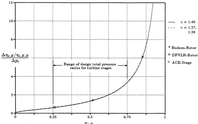
2.7 Total pressure loss and isentropic efficiency drop for a turbine . . . .

2.8 Total pressure loss and polytropic efficiency drop for a turbine . . . . .

2.9 Total pressure loss and isentropic efficiency drop for a compressor . . . .

2.10 Accuracy of the second-order entropy rise

(Q

2.11 Accuracy of the second-order entropy rise (n = 4) . . . .

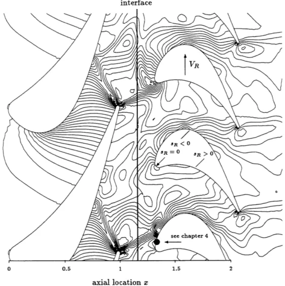
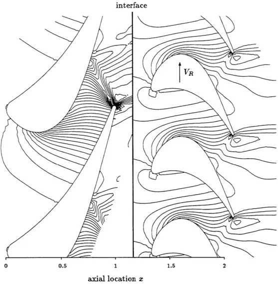
2.12 Static pressure contours in an unsteady simulation of the ACE turbine stage for (t/T ) = 0.7 . . . .

2.13 Static pressure contours in a steady simulation of the ACE turbine stage

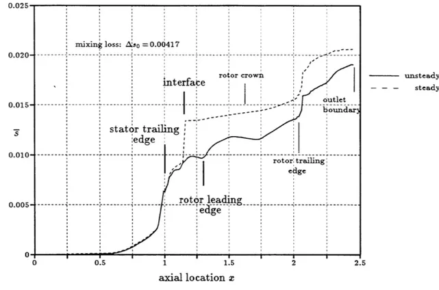
2.14 Entropy rise in the simulations of the ACE turbine stage . . . .

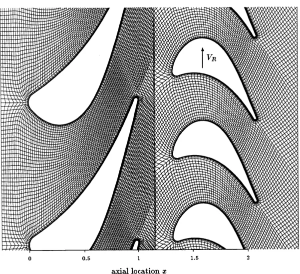
2.15 Stage geometry and computational grid of the ACE turbine stage for

(t/T ) = 0.7 . . . . 28 33 36 42 43 46 48 49 50 51 52 54 55 56 57

2.16 Decomposition of the entropy rise into the wave types and wavenumbers (fundamental wavenumber kyl corresponds to the stator pitch) . . . . . 58

3.1 An isolated airfoil with an unsteady lift and circulation . . . . 64

3.2 A cascade with an unsteady lift and circulation . . . . 68

3.3 Relative magnitude of the spatial harmonics in the shed vorticity wake (first harmonic corresponds to the pitch of the upstream blade row) . . 74

3.4 Relative amount of kinetic energy in higher spatial harmonics . . . . 75

4.1 Steady boundary layer subject to a discontinuous freestream velocity . . 87

4.2 Unsteady boundary layer on an oscillating wall . . . . 88

4.3 Unsteady boundary layer on a blade surface . . . . 89

4.4 Unsteady boundary layer on a blade - simulation of the ACE turbine stage at (t/T) = 0.9 . . . . 90

4.5 Unsteady streamwise velocity distribution as a function of the wall distance100

4.6 Dissipation rate for the 'exact' solution and the high-frequency limit . . 102

4.7 ht - s diagram for an ideal gas - revisited and magnified . . . . 103

4.8 Model problem for the numerical evaluation of modeling errors . . . . . 108

4.9 Comparison to Lighthill's analytic solution in laminar flow . . . .

4.10 Comparison between 'exact' numerical solution and high-frequency limit

4.11 High-frequency-limit model and 'exact' laminar model dissipation. . .

4.12 Comparison to Cousteix's experiment - unsteady streamwise velocity

112

113

114

4.13 Comparison to Cousteix's experiment - unsteady velocity phase . . .

4.14 High-frequency-limit model and 'exact' turbulent model dissipation -downstream propagating pressure waves . . . .

4.15 High-frequency-limit model and 'exact' turbulent model dissipation -upstream propagating pressure waves . . . .

4.16 Unsteady streamwise velocity distribution in a turbulent mean flow -upstream propagating pressure waves . . . .

4.17 Unsteady streamwise velocity distribution near the wall in a turbulent mean flow - upstream propagating pressure waves . . . .

4.18 Entropy rise per unit surface length on the ACE rotor . . . .

4.19 Attenuation of an acoustic wave in an unsteady boundary layer . . . . .

4.20 Average entropy in the rotor passage H-grid (the freestream) . . . . 117 118 119 120 121 124 130 134

4.21 Average entropy in the

0-grid

4.22 Time-mean rotor surface entropy . . . . 137

E.1 Eigenvectors for evanescent pressure waves in the complex plane . . . . 159

List of Tables

Contributions to the entropy rise at the interface - by wave type . . . 59

Contributions to the entropy rise at the interface - by wavenumber . . 60

Input parameters for the simulation of the Cambridge No.2 turbine . . 76

Unsteadiness parameters and results for the Cambridge No.2 turbine . 77 Input parameters for the LSRR simulation . . . . 78

Unsteadiness parameters and results for the LSRR . . . . 79

Input parameters for the DFVLR turbine simulation . . . . 80

Unsteadiness parameters and results for the DFVLR turbine . . . . 80

Input parameters for the ACE turbine stage simulation . . . . 81

Results for the ACE turbine stage . . . . 82

Input parameters for the NASA stage 67 simulations . . . . 83

Results for the NASA stage 67 simulations . . . . 84

4.1 Input parameters for the ACE turbine stage simulation . . . .

Modal contributions to the Unsteady Viscous Loss of the ACE rotor .

Isentropic efficiencies for the steady and the unsteady ACE simulation

123 125 127 2.1 2.2 3.1 3.2 3.3 3.4 3.5 3.6 3.7 3.8 3.9 3.10 4.2 4.3

Nomenclature

I

blade chord or blade axial chord blade axial chord

specific heat at constant pressure Euler's constant

total specific energy of a fluid, et = ht - (pIp)

jth unit vector, ej = [65

ij, 62 3j, 64j

total specific enthalpy of a fluid wave number,

reduced frequencies, defined in equation (3.5) or (4.6) length scale

temporal and spatial mean of the secondary kinetic energy polytropic exponent

coordinate normal to a blade surface pressure

heat

kinetic energy ratio, defined in equation (3.41) entropy,

blade surface coordinate

nondimensional time-mean mass-average entropy, defined in (2.36)

time

velocity in the direction of the coordinate x or s wall friction velocity, defined in (4.89)

velocity in the direction of the coordinate y or n eigenvector

axial coordinate

convected coordinate, in the mean flow direction circumferential coordinate

convected coordinate, normal to the mean flow coordinate in the direction of wave propagation

matrices in the Euler equations in primitive form, defined in (2.5) complex amplitudes of the potential functions (3.8) and (3.24) matrix to calculate the second-order entropy rise in (2.36) acoustic energy density, defined in equation (2.41)

flux vectors in the Euler equations, defined in equation (2.2) matrix to calculate second-order mean flow changes in (2.30) high-reduced-frequency limit A, B A, B D E F, G H HFL

I

N acoustic energy flux defined in equation (2.41)

M Mach number

P pitch

rotated pitch (in a convected coordinate system),

P

P* pitch of the neighboring blade row in a single stage

Pr Prandtl number

R square root of the discriminant defined in (2.16), specific gas constant

R acoustical impedance

Re Reynolds number

Re, Reynolds number defined with the local coordinate s

Re9 Reynolds number defined with the momentum thickness 0

S entropy flux in subsection 2.3.2, S = pus

T period,

characteristic time, temperature

Tf forcing time scale (blade passing period or an integer fraction thereof) U state vector defined in equation (2.2) or (2.5)

Ue freestream convection velocity VR rotor speed

Greek Symbols

a angle between the blade wake and the axial direction )3 inter-blade phase angle,

amplitude attenuation factor

18 inter-blade phase angle in a convected coordinate system -y ratio of specific heat for an ideal gas,

vortex sheet strength

6

bf unsteady boundary layer thickness

61 laminar sublayer layer thickness in turbulent flow b, viscous length scale

P* displacement thickness

6zi Kronecker delta function, defined in appendix C E small (perturbation) parameter

E₂, e4 second-difference and fourth-difference smoothing coefficients

efficiency

0 angle between the wave propagation direction and the surface normal

K thermal conductivity

A a reduced frequency defined in equation (3.22)

Af

V kinematic viscosity 7rt total pressure ratio

p density

a- normal stress

7' shear stress

rt

4>

<p phase angle

w angular frequency

Wf forcing frequency, blade passing frequency

I circulation

A difference,

small perturbation, grid spacing

<I> dissipation function, first defined in equation (4.14) fl reduced frequency defined in equation (2.11),

control volume, volume of integration dn control volume boundary

Others

R(

),

9()

V gradient operator

Subscripts

e at the boundary layer edge

i _integrated,

incoming

in at the inflow boundary

inv inviscid

1 left

M mth spatial/temporal harmonic

n

nth

in/normal to the direction of n

p in primitive form, polytropic

o fluid state after the dissipation of unsteady waves

out at the outflow boundary

r right,

reflected,

isentropic,

in/normal to the direction of s,

based on the local value of the coordinate s total/stagnation quantity,

turbulent

velocity in the direction of the coordinate x or s velocity in the direction of the coordinate y or n viscous

at the wall

in the direction of the coordinate x, in the direction of the coordinate y

S t U V Vis w y C D E HFL R S 0 1 2 3 4 0 00 Superscripts T

zeroth-order, mean state

first-order, first-order perturbation, entropy wave,

fluid state before compression

second-order, second-order perturbation, vorticity wave,

fluid state after compression

pressure wave propagating or decaying downstream, fluid state before expansion

pressure wave propagating or decaying upstream, fluid state after expansion

based on the momentum thickness at infiuty

transpose

quantity in a convected coordinate system unsteady quantity

complex amplitude

temporal mean, temporal and spatial mean vector quantity compression design expansion high-reduced-frequency limit rotor stator

Chapter 1

Introduction

Flow fields in turbomachinery are inherently unsteady, with a multitude of sources con-tributing. The incoming flow itself can be nonuniform resulting in an unsteady inflow to the rotor frame of reference. The relative motion of neighboring blade rows, in conjunc-tion with the spatially nonuniform pressure fields locked to loaded blades, leads to an unsteady pressure distribution in both through so-called potential interaction. A blade row may also move through and interact with shock wave systems. Stator wakes con-vected with the mean flow cause unsteadiness in the rotor frame of reference. Similarly, secondary flow effects like horse shoe vortices, passage vortices, and tip clearance vor-tices contribute to flow unsteadiness. The viscous flow past a blunt turbine trailing edge results in vortex shedding; trailing-edge vortex shedding has also been found in com-pressors operating in the transonic or supersonic regime. Finally, there is unsteadiness induced by the motion of the blades themselves, i.e. blade flutter.

Very successful turbomachines have been developed in the past by compensating for the lack of basic knowledge about unsteady effects or for their neglect with extensive empirical correlations. The past two decades have seen a strong increase in the experi-mental and computational effort devoted to unsteady flows in turbomachinery. Partly, this increase was driven by a tremendous rise in the computing power and memory available and by new or improved experimental facilities and techniques. Partly, it was fueled by continuing demands to improve upon existing designs and design methodolo-gies. To increase engine efficiencies and stability margins, to extent engine life-times, to reduce weight and size, and to cut development cost and time, it is imperative to study and understand unsteady flow phenomena. With turbomachinery efficiencies typically around 90%, there is room left for improvement but one needs to look at all sources of loss, including those considered too small or too difficult to treat before.

1.1

Motivation

Besides the general recognition of the importance of unsteady effects in turbomachinery, several specific factors motivated this thesis.

First among them is the continuing prevalence of steady tools for routine design purposes in industry. The standard aerodynamic design tools for turbomachinery are steady codes, both inviscid and viscous, and steady cascade experiments. Designing a single stage or blade row with steady-state tools amounts to placing the stator and rotor row infinitely far apart thus eliminating the effects of blade row interaction. Un-steadiness, however, contributes additional loss with non-zero time-meant First, most of the energy associated with the unsteady part of the flow field is not recovered; it will eventually be dissipated. Second, the interaction of unsteadiness with boundary layers and shock structures can trigger additional loss. In a steady viscous simulation, the effect of unsteadiness on the efficiency is not captured. An unsteady, nonlinear simu-lation is still prohibitively expensive for routine design purposes and will likely remain so in the foreseeable future, particularly for multistage turbomachinery. Testing of a stage or a whole turbine under unsteady operating conditions will remain impractical for routine design purposes. Therefore, the error in the predicted efficiency stemming from the neglect of unsteady effects needs to be assessed.

Recently, linear perturbation methods have received increased attention as alterna-tives to fully nonlinear, unsteady simulations. In linear CFD-codes, a nonlinear steady state is found and the unsteady flow field is superimposed as a small perturbation. Second-order terms, i.e. terms quadratic in unsteady quantities, are neglected since the perturbations are assumed to be small. Linear perturbation codes have been found to give accurate results up to a surprisingly high level of unsteadiness [1, 2] and will be more widely used in the future. Linear codes, like steady codes, cannot capture un-steady loss. The time-mean of the first-order unun-steady dissipation is zero; only terms second-order in unsteady quantities have a non-zero time-mean.

'This is not meant to imply that an increased spacing increases the efficiency. See sections 1.2 and 2.7 for a further discussion of this point.

Most recently, CFD-codes have been developed which account for the second-order effect of unsteadiness on the time-mean flow. Work in this direction has been pursued by Adamczyk [3] and Giles [4]. In this context, the thesis research was intented to underscore, or not, the need to include these effects.

Fully nonlinear, unsteady, viscous CFD-codes are another tool to evaluate unsteady loss. However, the weakest point of any numerical simulation, steady or unsteady, remains the accurate prediction of heat loads and losses due to the unavailability of adequate turbulence and transition models. Thus, there is a need to examine the mod-eling accuracy of numerical simulations with respect to unsteady flow phenomena and unsteady losses. Throughout this thesis research, the CFD-code UNSFLO by Giles

[5, 6, 7], and the visualization package VISUAL2 by Giles and Haimes [8] were used.

The turbomachinery community is moving towards the consensus that increased losses under unsteady operating conditions are primarily due to strongly nonlinear ef-fects like the alteration of the boundary layer characteristics through their effect on transition [9], the variation of secondary flow generation in downstream blade passages, and their effect on separation or reattachment. Those effects are beyond the realm

of the linear/quadratic approach taken in this thesis. Nevertheless, the magnitude of effects that can be treated in a linear framework, remains to be determined.

1.2

Unsteadiness and Loss

-

Historical Perspective

Theoretical and Experimental Work

Unsteadiness affects the efficiency of turbomachinery in a variety of ways. What follows is a necessarily incomplete list of subjects of past investigations.

One of the earliest investigations was done by Keller [10] in 1935, who considered the transfer of mean-flow energy to the unsteady flow field through shedding of vorticity in an incompressible flow. The vorticity is shed off the blade trailing edges in response

to circulation variations, and its kinetic energy cannot be recovered. Keller estimated the circulation amplitudes and concluded that the rate of energy transfer is equivalent to between 0.4% and 1% of the power delivered or consumed by the rotor. In 1955, Kemp and Sears [11] applied thin-airfoil theory developed earlier [12, 13, 14], and used in the approximate analysis of interference between blade rows [15], to calculate the circulation variations, the shed vorticity, and the associated kinetic energy. They ar-rived at the conclusion that the rate of energy transfer is, generally, much less than estimated by Keller. In 1973, Hawthorne [16], who used a lifting-line approach, found rates of energy transfer which are in line with those of Keller[10].

In 1970, Kerrebrock and Mikolajczak [17] advanced a wake transport model to ex-plain experimentally observed stagnation temperature and pressure non-uniformities in the stator exit plane of a compressor stage and their effect on the performance. In 1984, Ng and Epstein [18] measured large total temperature and pressure fluctuations at three to four the times blade passing frequency in the rotor core flow of a compressor stage. They proposed a moving shock model coupled to shed wake vorticity to explain their origin and deduced the magnitude of the associated loss. The entropy rise due to a moving shock was found to lead to a 0.15% drop in the efficiency while the mixing-out of fluctuations led to a loss on the order of the wake loss. Additional losses were expected from the interaction of the shed vorticity with downstream shock structures. Experi-mental evidence for moving shocks in a compressor rotor has subsequently been found by Strazisar [19]; Hathaway et el. [20] found vortex shedding in a axial-flow fan. Owen [21] observed vortex shedding off a transonic compressor rotor in numerical simulations.

More than one source of unsteadiness affects the compressor performance upon vari-ation of the blade row gaps; those include wake transport, potential interaction, and wake mixing, among others. In 1970, Smith [22] reported an efficiency increase of 1% for reduced gaps in an multistage compressor. Later, Mikolajczak [23] confirmed their find-ings, while experiments by Hetherington and Moritz [24] contradicted them; the above experiments suggest that choosing an aerodynamically optimal gap is not an easy task.

The first studies on the influence of unsteadiness on the profile loss and the effi-ciency in attached flows appeared in the late sixties and early seventies [25, 26, 27]. Obremski and Fejer [28], as well as Walker [29], observed early transition in unsteady flow, leading to a greater length of the blade surface being covered by turbulent flow. Pfeil et al. [30, 31] observed unsteady transition on a flat plate subject to periodic wake-type disturbances. The same transition mechanism was found in an axial-flow compressor by Evans

[32],

Numerical Developments

The progress in the numerical simulation of unsteady flow over the past two decades has been impressive. The range of methods includes linear potential [36, 37] and linear Euler methods [1, 2, 38], as well as nonlinear codes solving the Euler [5, 6, 39, 40, 41, 42, 43] or the Navier-Stokes equations [7, 44]. In linear (perturbation) methods, the steady flow is a solution to the nonlinear potential equation or to the nonlinear Euler equations, and the unsteady flow field is superimposed as a small perturbation. The appeal of linear methods lies in the savings in CPU-time they offer over a fully nonlinear formulation.

In response to the impracticality of multistage, unsteady, viscous simulations, Adam-czyk [3] formulated a system of equations to account for the time-mean effect of the de-terinnistic periodic unsteadiness on the mean flow through second-order terms similar to Reynolds stresses. In a research project related to this thesis, Giles [4] developed an asymptotic approach to unsteady flow in multistage turbomachinery. The asymptotic parameter is the level of unsteadiness in a flow described by the Euler equations. The approach leads to separate equations for the mean flow, the first-order perturbations, and the time-mean of the second-order perturbations. These can be solved more effi-ciently than the full nonlinear equations, in particular for multistage turbomachinery.

A number of comparisons have been conducted between experiments and simula-tions. Those were focusing, for example, on wake/stator interaction [5, 9, 42, 45], on the redistribution of inlet temperature profiles in a turbine stage

[46,

1.3

Thesis Outline

The first component of this thesis, chapter 2, focuses on the relation between unsteadi-ness and loss in two dimensions. The unsteady waves that are solutions to the linearized Euler equations are entropy and vorticity waves, convected with the mean flow, and pres-sure waves of propagating or evanescent nature. Concluding that most of the energy associated with the unsteadiness cannot be recovered, an asymptotic analysis in sec-tion 2.3 yields the second-order mean flow change and entropy rise resulting from the dissipation of an arbitrary combination of unsteady waves in a uniform mean flow. For the use in subsequent chapters, section 2.5 links the entropy rise to a total pressure loss and to a change in performance through a linearization of the isentropic efficiency. The result of the analysis is used in section 2.6 to evaluate the accuracy of the linear approach, and in section 2.7 to analyze mixing loss at the stator/rotor interface of a steady simulation.

The second component of this thesis focuses on the nature and the location of unsteady loss mechanisms and the magnitude of the associated losses. Two aspects are covered, termed Unsteady Circulation Loss and Unsteady Viscous Loss, respectively.

Chapter 3 revisits the Unsteady Circulation Loss first treated by Keller [10] in 1935 and later by Kemp and Sears [11] in 1956. Keller estimated the unsteady circulation amplitude to arrive at the kinetic energy in the unsteady flow field induced by the shed vorticity. Sears and Kemp used thin-airfoil theory to obtain the unsteady circulation amplitude. This approach, while enabling them to calculate the circulation amplitude,

limited them to incompressible flow and blades of zero thickness and camber with the mean flow nearly in the blade direction, i.e. lightly loaded blades. Thus, the airfoils are more representative of compressor blades than turbine blades. In this thesis, the circulation amplitudes are obtained from numerical simulations, which allows one to obtain amplitudes for arbitrary blade and stage geometries, steady lift distributions, and Mach numbers. Kelvin's Circulation Theorem, upon which Keller's work rests, is valid even in compressible flows, provided they are homentropic. Eliminating the need to estimate the circulation amplitudes or to deduce them from thin-airfoil theory, results in a realistic measure for the secondary kinetic energy in modern turbomachines and

the loss associated with its dissipation.

The unsteady stator/rotor interaction can generate strong pressure waves. Unsteady Viscous Loss, considered in chapter 4, is a consequence of dissipation in unsteady bound-ary layers driven by these pressure waves. Using a linear approach and a near-wall ap-proximation in the high-reduced-frequency limit, the streamwise momentum equation, driven by unsteady pressure gradients, yields the local velocity distribution in the lam-inar Stokes' sublayer. The driving pressure gradients are obtained from an unsteady simulation. In the high-frequency limit, the dissipation in unsteady boundary layers depends only on the unsteady shear. The associated entropy generation is integrated over a blade surface and related to a drop in the isentropic efficiency. The result of a numerical study to check the errors introduced by a departure from the high-frequency limit is presented in section 4.3. Section 4.4 applies the loss model to a transonic tur-bine stage and discusses the modeling accuracy of numerical simulations with respect to unsteady loss.

Chapter 5 summarizes the approaches taken and the results obtained in this thesis, and gives recommendations for future research on the topic of unsteady loss.

Chapter 2

Unsteadiness and Loss

The objective of this chapter is to establish, in a rigorous mathematical manner, a link between the dissipation of unsteadiness in a two-dimensional, inviscid, compressible flow and the efficiency of turbomachinery. The result will be used in the investigation of unsteady loss mechanisms in chapters 3 and 4, and in discussions of the numerical modeling accuracy.

The unsteady waves that are solutions to the linearized Euler equations in two dimensions are entropy and vorticity waves, convected with the mean flow, and pressure waves of propagating or evanescent nature. They are briefly (re)derived in section 2.1; this section closely follows [55]. Section 2.2 contains a brief survey of literature on wave transmission and reflection in turbomachines and takes a short look at the rectification of energy associated with unsteady waves.

A novel asymptotic analysis in section 2.3 links unsteady waves to the loss resulting from their dissipation in a uniform mean flow. In subsection 2.3.1, a mathematically rigorous flux-averaging procedure for an arbitrary unsteady flow relates the dissipation of unsteady waves to second-order mean-flow changes. Subsection 2.3.2, in turn, relates the change in the mean state vector to a time-mean mass-average entropy rise. It emphasizes the separate contributions from waves of different frequency, wavenumber and physical nature. Section 2.5 relates the entropy rise to an equivalent total pressure loss and to a change in the turbomachine performance through a linearization of the isentropic efficiency.

Section 2.6 looks at the accuracy of the second-order entropy rise calculated from the linear model by comparing it to the entropy rise calculated with a nonlinear approach. Section 2.7 contains the first application of a linear/quadratic model to the analysis of the interface treatment (the mixing loss) in steady rotor/stator interaction simulations.

2.1

Unsteady Modes

In the core flow, the inflow and outflow boundaries, and the gap between blade rows of a turbomachine, the Euler equations are sufficient to describe the fluid motion. They are usually expressed in a form based on the conservation of mass, momentum, and energy.

8U aF 9G

+ +- =0 (2.1)

The state vector U and the flux vectors F and G are defined by

Pu pv

Pu Pu2

₊

U = , F = , and G= . (2.2)

pv puv Pv2_+p

.pet , puht j L

pvht

The pressure is determined from

p = ( p-1) Pet - p (u2 + V2 , (2.3)

where - is the (constant) ratio of specific heats. Equation (2.3) can be used to eliminate the total energy per unit mass, et, and the stagnation enthalpy, ht = et + (p/p), from equations (2.1) to obtain the Euler equations in the so-called primitive form.

Up + U BU

-+A "+B -=0 (2.4)

at Ox ay

The primitive state vector U, and the matrices A and B are defined by

P' u p 0 0 V 0 p 0

u 0 u 0 1/p 0 V 0 0

U,= _V , A = ₀ 000 _{0 U} ,and B = 00 v./ (2.5)

0 0 0 V 1/p

.P. 0 7P 0 u . . 0 0 7YP v _

Equations (2.4) are still nonlinear; they are linearized by considering small perturbations

EU1

Up = UO + fUi (X, y, t) + ... (2.6) Since the character of the flow depends on the mean Mach number M ,O, it is advanta-geous to nondimensionalize the mean flow and the unsteady perturbations by the mean

density po and the mean speed of sound ao. equations (2.4) are with U1, A0, a 1 9U1

au

at+

AO

X

U

0

0

0

0

L 0

The first-order perturbations of the Euler

aU

1

0

0

0

0

0

0

0

0

Searching for wave-type solutions

U1(x, y, t) = U(x, y, t) = -, exp {i (k,,x + kyy - ot)}

to equation (2.7), one is led to

- + Ao +Bo , = 0,

where 5,. is a right eigenvector; the reduced frequency f is defined as

From the definition of AO and BO, the dispersion relation is found as

k ,o + MyO - Q (2.9) (2.10) (2.11) (2.12) kXMXO + My'O - 2 = 0. (kxM

With the reduced frequency S and the circumferential wavenumber k. known, tion (2.12) may be solved for the axial wavenumbers k,, i.e. the eigenvalues of equa-tions (2.7). The corresponding right eigenvectors are determined from equation (2.10).

k 2 k2 Y

The first two eigenvectors correspond to the twofold eigenvalue

k.,1 =k.,2 = ky '' (2.13)

MX'0

The corresponding eigenvectors are not unique and are chosen as

0 -M

0

W-,1= and 1,,2 = . (2.14)

0 JL 0

The first right eigenvector, with a perturbation in the density only, represents an entropy wave, while the second, with perturbations in the velocities only, represents a vorticity wave. Both are convected with the mean flow.

The third and fourth eigenvector correspond to the eigenvalues

kx,/4= -y(fl - My,o) ( R - M--,o) (.5

1 M2 _(2.15)

where

R= 1 - - MX,' .,) (2.16)

(f2- MY,0)2'

For a negative discriminant of R, the root with the positive imaginary part is implied. The corresponding eigenvectors are

- (f - My,o) ( Mx,oR - 1)

(1 - My,o) ( R - Mx,o)

Wir,3/4 = .

M,0 (2.17)

L (n - My,o) ( Mx,oR - 1)J

In axially subsonic flow (IMx,oI<1), they represent (isentropic) evanescent pressure waves with amplitudes decaying axially upstream and downstream, if the reduced frequency falls in the range

(M',o

Q

eigenvectors represent (isentropic,) propagating pressure waves. In axially supersonic flow

(IMx,oJ

2.2

Dissipation and Rectification

In section 2.1, the unsteady waves that are solutions to the linearized Euler equations have been briefly rederived. The unsteady waves generated by wake/blade row in-teraction, rotor/stator inin-teraction, vortex shedding, or any of the other mechanisms described in the introduction, propagate and/or are convected through the blade rows of a turbomachine. Away from the blades, the Euler equations are sufficient to describe the convection and propagation of unsteady waves, even if their origin is viscous as is the case for blade wakes or the vorticity shed off a blunt turbine trailing edge. The amplitudes of the unsteadiness in a turbomachinery environment can be quite large, in particular in the presence of viscous wakes and shock waves. Wakes are decomposed into vorticity and entropy waves while the weak shock waves can be modeled as isentropic pressure waves.

Unsteady waves in a turbomachine will undergo one of the following processes: " Rectification

" Laminar or turbulent dissipation (in the blade passage or in boundary layers) " Radiation out of the turbomachine upstream of the first row in an

unchoked turbomachine

" Outflow or radiation out of the turbomachine downstream of the last blade row " Acoustic transmission to the environment through the structure

" Dissipation through structural damping

Rectification denotes the recovery of energy associated with unsteady waves through its transfer to the mean flow. The effect of acoustic transmission and structural damping (an important player in the phenomena of flutter and forced response) cannot easily be quantified; they are not considered here. In multistage turbomachines one would expect the outflow/radiation at the inlet or the outlet to play a minor role only. In single-stage turbomachines, energy associated with unsteady waves is convected or radiated out and eventually dissipated. For multistage turbomachines, this leaves viscous dissipation in

the blade passage, the gap, and in unsteady boundary layers at blade, hub and tip as primary loss mechanisms.

Excluding the extraction of extra energy from the mean flow by unsteady waves, there are three questions about the effect of unsteadiness on the efficiency of turbo-machinery. First, there is the question as to what percentage of the energy associated with unsteadiness is lost and what percentage is rectified. The second question pertains to the loss mechanism and its locus, if rectification is not possible. The third question inquires about the associated loss. Subsection 2.2.1 will briefly touch on the issue of rec-tification while subsection 2.2.2 takes a short look at the literature on wave transmission and reflection to make a conclusion about the locus of dissipation.

2.2.1 Conditions and Mechanism for Rectification

(k,)

IVR

stator row interface rotor row

Figure 2.1: Rectification of unsteady waves

The energy associated with an unsteady wave can be rectified if the wave becomes steady in the rotor frame of reference. Figure 2.1 illustrates this process. An unsteady wave with normal wavenumber and frequency (k., w) in the rotor frame crosses into the stator frame of reference. There, it is perceived as a wave with the same wavenumber but a different frequency due to the relative motion of the blade rows. Reflection at the stator blade row will give rise to waves of the same frequency but differing in their

wavenumbers by a term (2rn/Ps), where Ps is the stator pitch. Crossing back into the stator frame of reference, they keep their wavenumbers but shift their frequencies to (w+27rnV/Ps). If

w

To recover the energy of a wave which is unsteady in the rotor frame and convert it into mechanical energy, the following conditions must hold:

e

of the unsteadiness

The first condition implies that the effect of a wave on different rotor blades in a row must be identical. Otherwise, the compound effect of the individual blade lift varia-tions is zero; lift variavaria-tions of different blades cancel. In practice, turbomachines never have identical rotor and stator pitches, making it impossible that the circumferential wavelength and the rotor pitch match. The second condition is of similar nature. If the wavelength is short compared to the blade chord, variations over different parts of a blade have a zero net effect on the blade lift. The third condition states that any lift circulations must be quasi-steady compared to the inertial time scale of the rotor. Oth-erwise, the rotor speed cannot follow lift variations and increase the mechanical energy delivered at the shaft. In turbomachines, the inertial time scale is much larger than the unsteady waves periods (which are linked to the blade passing frequencies and their harmonics), ruling out the rectification of waves which are unsteady in the rotor frame.

2.2.2 Wave Transmission and Reflection

Pressure waves encountering a blade row are partly transmitted and partly reflected. As a consequence of the Kutta condition, a vorticity wave is shed at the trailing edge of every blade. When a vorticity wave impinges upon the leading edge of a blade row, pressure waves are generated and another vorticity wave is shed at the trailing edge. Amiet

[56]

The amount of energy dissipated in the turbomachine and the location of its dissi-pation depend on the transmission and reflection characteristics of the blade rows with respect to the unsteady waves impinging upon them. The larger the reflection coeffi-cients in a multistage turbomachine, the more likely it is that the waves are dissipated

in place, i.e. in the gap between the blade rows or in unsteady boundary layers on the

adjacent blade rows. Also, the larger the reflection coefficient of the blade rows, the larger is the probability that unsteady waves become steady in one frame of reference and are rectified. The larger the transmission coefficient, the more likely it is that they are radiated or convected out at the upstream or downstream end of the turbomachine.

Kaji and Okazaki [57, 58] made the most thorough study of this problems with a minimum number of limiting assumptions. In [57], they used a semi-actuator disk model to determine the transmission and reflection coefficients of a single blade row for a plane pressure wave or a vorticity wave impinging from upstream and for a plane pressure wave impinging from downstream. They examined the effects of mean-flow Mach number, wavelength, incidence angle, stagger angle, and steady aerodynamic blade loading. The Mach number and the incidence angle, combined with the stagger angle, were found to be the most important factors in determining the coefficients. High subsonic Mach number and angles of incidence far from the stagger angle substantially increased the reflection coefficients. The ratio of the wavelength of the incident wave to the blade chord had a minor effect only, especially at higher Mach numbers. The steady aerodynamic loading, i.e. the introduction of turning, was without substantial effect, its tendency being to increase the reflection coefficient and to eliminate cases of pure transmission or reflection. In a second paper [58], they used an acceleration potential method to clarify the effect of finite blade spacing; typically the longest wave in a turbomachine has a wavelength on the order of a blade chord or a blade pitch. It was found to be most significant at low Mach numbers and of secondary importance at high Mach numbers.

Muir

[59]

three dimensions and cambered blades. The model is limited to circumferential wave-lengths which are long compared to the blade spacing. The effect of three-dimensionality was found to be slight over the whole range of Mach numbers and cascade parameters.

Grooth

[60]

in numerical simulations.

In all the references considered, the values of transmission and reflection coefficients varied greatly, depending on the exact choice of parameters like Mach number or angle of incidence and stagger. To draw a conclusion about the relative importance of trans-mission versus reflection, and ultimately about the locus of dissipation, these parameters would have to be known. None of the references treated camber angles close to those commonly found in turbines, nor did any of them consider the effect of blade-thickness. The results are therefore more relevant for compressors than for turbines. No clear general conclusion can be drawn about the reflection and transmission characteristics of blade rows in turbomachines; the exact amount of energy (associated with unsteady waves) rectified or dissipated, as well as the locus of dissipation, remain unknown.

2.3

Loss Due to Dissipation of Waves

The references on wave transmission and reflection examined in subsection 2.2.2 did not provide a clear picture of the relative importance of these phenomena or the applicability of the results to turbines. While some of the energy (associated with unsteady waves) can be recovered because they become steady upon changing the frame of reference, as illustrated in subsection 2.2.1, no quantitative assessment is available. The restrictive

conditions placed on rectification suggest that little of this energy can be recovered.

If the energy of unsteady waves is simply lost (rather than causing extra unsteady losses), the level of loss still depends on the mean flow state at the locus of dissipation.

Part of the energy dissipated into heat at a pressure level above the exit pressure can be recovered in downstream blade rows. Downstream of a single-stage or a multistage turbomachine, the locus of dissipation and the mean flow state are obvious. In general, the locus of dissipation and the associated mean flow state are unknown.

Nevertheless, it is important to ask how an unsteady wave, or a combination thereof, contributes to the loss upon its dissipation in an arbitrary but uniform mean flow. There-fore, this section proceeds to investigate the dissipation of an arbitrary combination of unsteady waves in an arbitrary constant mean flow. The emphasis is on the final mag-nitude of the (mixing) loss as a result of complete spatial and temporal averaging of waves rather than its spatial evolution. By its nature, the result is directly applicable only to the generation of mixing loss downstream of the last blade row of a turboma-chine and to the (unphysical) generation of loss at the interface in steady rotor/stator interaction simulations.

2.3.1 Flux-Averaging

A novel asymptotic approach and a control-volume argument are central to the analysis. Its aim is to link the dissipation of unsteady waves in a uniform mean flow to a measure

of loss. Figure 2.2 serves to illustrate the idea.

At the right-hand side, the outflow boundary, the uniform and steady mean flow is described by the state vector in primitive form, Uo.

U,,- = UO (2.18)

At the left-hand side, the inflow boundary, the spatially and temporally varying flow enters the control volume. The flow there is described by

U,,b ( , yi o) = UO + A U ( I Y, T . (2.19)

by an asymptotic expression in the small parameter E.

AU (X, y, t) = EU1 (X, y, t) + E2U2(X, y, t) + - - - (2.20)

The first-order perturbations, U1

(x,

[4]

y

6

Q

L

.X

Figure 2.2: Control volume for the asymptotic analysis

The two-dimensional Euler equations in integral (conservation) form are

dd

- UdA + f(Fdy _{+Gdx) =0.}

dt dog (2.21)

Applying them to the control volume depicted in figure 2.2 and integrating over one fundamental period in time and space, one obtains the equations

Pout = Fin, (2.22)

where

(i)

} ft

[i

series expansion for the components of the flux vector, Fj, yields

Fj (Uo + AU) = Fj (Uo) + d AU+ I AUTdFj AU+ - (2.23)

dUp

The second derivative of the flux vector, !-, is a third-order tensor; the second deriva-tive of a flux vector element F, dU-, can be expressed as a matrix, though. To check the derivatives, Mathematica@, a software package for performing symbolic mathemat-ical manipulation by computer, was used. The first and second derivatives of the flux vector are defined in appendix A. Substituting the asymptotic expression (2.20) into (2.23), one obtains

d Fj

F3 (Uo + AU) = Fj (Uo) + c U1

UP=Uo

+f21 UTd2

F

+

1

-

2 _dU

dU

Upon averaging, the second term on the right hand side of (2.24) vanishes because it varies harmonically iny time and/or circumferentially; all that remains is

-1

d

_Fi

_dFg

1

Fj (Uo + AU) = Fj (Uo) + E2 UF U1 + U2 + -2-+ - (2.25)

.2 d U _{dUp y_}

Equating fluxes as in (2.22), one obtains

21TdF ₃ dF

1

E -UTU 1 + _U2 + -- =0. (2.26)

2 dU _dU

From (2.26), one can calculate U2, the time-mean part of U2, by equating

second-order terms. Again, Mathematica® was used; this time to solve the linear system of equations (2.26) for U₂.

- -2

- 1 dF Ed2 UT Fj

U2 = U1 (2.27)

2dp U,=UO _ j=1 dUP U,=UO

The vector

4.

frequencies, wavenumbers, and physical nature.

4

U1 =

Um

m n 1=1 m n

The variable b denotes a real amplitude, and the variable <p a phase angle; t,.,i stands for the right eigenvectors defined in section 2.1. The real part is implied wherever complex quantities appear in place of physical variables. Due to the orthogonality properties of sines and cosines, listed in appendix C, the integration (or averaging) removes crosscoupling between modes of different circumferential wavenumbers ky,m or different frequencies w. Thus, one can consider one circumferential wavenumber and one frequency at a time and use the principle of superposition to obtain U2.

- 1 dF ej _d2

F m _(2.29)

U2 = 2 dU d2.29m"l

d~pyyo_ g apU=U

However, this does not remove crosscoupling between waves of different physical nature,

like

U2= -- ZUM"Hgj Umn. (2.30)

,0

g

The matrices H, are defined in appendix A.

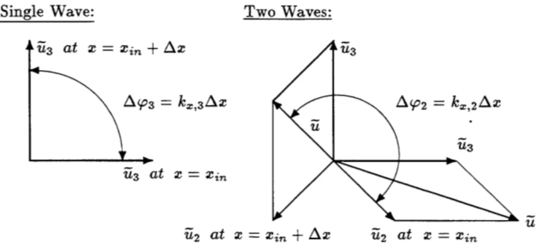
At this point, it is appropriate to remark that U₂,mn is a periodic function of the axial location of the inflow boundary due to the superposition of waves of different physical nature which are contained in U1, defined equation (2.28); the mean inflow

state, U,,in = UO +U 2, varies periodically in the axial direction. This holds true even

though one only considers waves of one circumferential wavenumber and frequency.

If only one type of wave, for example a propagating pressure wave, is present, only the phase angles of the unsteady perturbations will vary with the axial location. When two or more waves are present, the amplitude as well as the phase of the compound perturbation can change with the axial location! Figure 2.3 illustrates this for