Balancing actuation energy and computing energy in low-power motion planning

Balancing Actuation Energy and Computing Energy

in Low-Power Motion Planning

by

Soumya Sudhakar

B.S.E., Princeton University (2018)

Submitted to the Department of Aeronautics and Astronautics

in partial fulfillment of the requirements for the degree of

Master of Science in Aeronautics and Astronautics

at the

MASSACHUSETTS INSTITUTE OF TECHNOLOGY

May 2020

c

○ Massachusetts Institute of Technology 2020. All rights reserved.

Author . . . .

Department of Aeronautics and Astronautics

May 19, 2020

Certified by . . . .

Sertac Karaman

Associate Professor of Aeronautics and Astronautics

Thesis Supervisor

Certified by . . . .

Vivienne Sze

Associate Professor of Electrical Engineering and Computer Science

Thesis Supervisor

Accepted by . . . .

Sertac Karaman

Chairman, Department Committee on Graduate Theses

Balancing Actuation Energy and Computing Energy in

Low-Power Motion Planning

by

Soumya Sudhakar

Submitted to the Department of Aeronautics and Astronautics on May 19, 2020, in partial fulfillment of the

requirements for the degree of

Master of Science in Aeronautics and Astronautics

Abstract

Inspired by emerging low-power robotic vehicles, we identify a new class of motion planning problems in which the energy consumed by the computer while planning a path can be as large as the energy consumed by the actuators during the execution of the path. As a result, minimizing energy requires minimizing both actuation energy and computing energy since computing energy is no longer negligible. We propose the first algorithm to address this new class of motion planning problems, called Computing Energy Included Motion Planning (CEIMP). CEIMP operates similarly to other anytime planning algorithms, except it stops when it estimates that while further computing may save actuation energy by finding a shorter path, the additional computing energy spent to find that path will negate those savings.

The algorithm formulates a stochastic shortest path problem based on Bayesian inference to estimate future actuation energy savings from homotopic class changes. We assess the trade-off between the computing energy required to continue sampling to potentially reduce the path length, the potential future actuation energy savings due to reduction in path length, and the overhead computing energy expenditure CEIMP introduces to decide when to stop computing. We evaluate CEIMP on real-istic computational experiments involving 10 MIT building floor plans, and CEIMP outperforms the average baseline of using maximum computing resources. In one rep-resentative experiment on an embedded CPU (ARM Cortex A-15), for a simulated vehicle that uses one Watt to travel one meter per second, CEIMP saves 2.1-8.9× of the total energy on average across the 10 floor plans compared to the baseline, which translates to missions that can last equivalently longer on the same battery. As the the energy to move relative to the energy to compute decreases, the energy savings with CEIMP will increase, which highlights the advantage in spending computing energy to decide when to stop computing.

Thesis Supervisor: Sertac Karaman

Title: Associate Professor of Aeronautics and Astronautics Thesis Supervisor: Vivienne Sze

Acknowledgments

First and foremost, I would like to thank my advisors, Vivienne Sze and Sertac Karaman, both of whom have given me so much guidance, insight, and hours of conversations on robotics and life. I am deeply grateful for the opportunity to work with you both, and it is an experience I have truly enjoyed. Thank you for introducing me to the fascinating field of low-power robotics and helping me grow into a researcher! I also would like to take the time to thank Janice Balzer for helping coordinate lab meetings, and Jin Gao, for her kindness and patience when helping me order items for research. Jin, thanks for going on an adventure with me to hunt down a pair of miniature motors in a FedEx facility, I am so grateful. I would also like to the AeroAstro, LIDS, and MIT staff for making the learning environment so enriching.

To my labmates both in LEAN lab and EEMS lab, grad school wouldn’t be nearly as fun without you all to share the journey. Thank you for the wonderful conversations, helpful feedback, and lab meetings that feel like family dinners. I would also like to thank the new friends I have made at MIT and around Boston, who made the moments in and out of the lab so filled with joy these last two years, and who even entertain the idea of a 24-hour celebration! Thank you and looking forward to the day we all reunite again.

To Andres Sisneros, thank you for making Boston feel so magical. Your support, encouragement, and zen mastery have meant so much to me during this grad school adventure, and I am excited for many more adventures together in the future. And of course, to my sister and my parents, your unconditional love, support, and belief in me means everything. Thank you for always encouraging me to chase my dreams, follow my passion, and do good in the world.

Finally, I have written this thesis during the unprecedented times of the coron-avirus pandemic. While these are uncertain times, what I know for sure is the bravery, sacrifice, and kindness shown by front line workers from health care professionals to the cashiers at my local grocery store. You all are my heroes, and without you, I would not have been able to write this thesis. With deepest gratitude, thank you!

Contents

1 Introduction 15

1.1 Overview of Low-Power Robotics . . . 15

1.2 Total Energy of Motion Planning . . . 17

1.3 Background on Motion Planning . . . 19

1.4 Related Work . . . 24

1.5 Thesis Contributions . . . 26

2 Modeling the Low-Power Motion Planning Problem as an MDP 29 2.1 Minimizing Total Energy in Motion Planning as a Stopping Problem 29 2.2 Markov Decision Processes and Dynamic Programming . . . 32

2.2.1 Modeling Low-Power Motion Planning as an MDP . . . 34

2.3 The Value of Continuing to Compute . . . 36

2.3.1 Backward Recursion for Finite-Horizon MDPs . . . 37

2.3.2 Approximate Dynamic Programming . . . 37

2.4 Summary . . . 38

3 Modeling Homotopic Class Changes in Motion Planning 41 3.1 Challenges in Predicting Homotopic Class Change . . . 41

3.2 Exploring Obstacle Space . . . 42

3.3 Occluded Graph as a Stochastic Shortest Path Problem . . . 44

3.4 Estimating the Probability of Repairs in an Occluded Graph . . . 47

3.4.1 Sampling Deterministically from a Distribution of Environments 48 3.5 Summary . . . 51

4 Don’t Think Too Hard: An Algorithm for Computing Energy

In-cluded Motion Planning 53

4.1 Algorithm Overview . . . 54

4.2 Solving CEIMP as an MDP . . . 56

4.3 Estimating Expected Future 𝐸𝑐 . . . 56

4.4 Estimating Expected Future 𝐸𝑎 from Local Optimization . . . 57

4.5 Estimating Expected Future 𝐸𝑎 from Homotopic Class Changes . . . 57

4.5.1 Occluded Graph Construction . . . 58

4.5.2 Estimation . . . 59

4.5.3 Expected-A* Algorithm to Approximate SSP Solution . . . . 61

4.6 Summary . . . 63

5 Analysis of Performance 65 5.1 Inclusion of Computing Energy in Cost Function . . . 65

5.1.1 Lack of Asymptotic Optimality . . . 65

5.1.2 Challenge in Proving Optimality of an Algorithm . . . 66

5.2 Complexity . . . 68

5.3 Convergence of Estimates on 𝐶𝑓 𝑟𝑒𝑒 . . . 69

5.3.1 Completeness of the Occluded Graph . . . 70

5.3.2 Convergence of Bayes Filters to True Edge States . . . 71

5.4 Error Bounds on Approximation to Stochastic Shortest Path Problem 71 5.4.1 Bounds on Expected-A* Compared to Value Iteration . . . 72

5.4.2 Correctness of Expected-A* . . . 73

5.5 Summary . . . 74

6 Experimental Evaluation 75 6.1 Methodology . . . 75

6.2 Experimental Results . . . 78

6.2.1 Reductions in Total Energy . . . 78

6.2.2 Effect of Computing Efficiency on CEIMP Performance . . . 82

6.2.4 Overhead Evaluation . . . 84 6.3 Summary . . . 86

List of Figures

1-1 Examples of low-power platforms [1, 2, 3, 4, 5, 6, 7, 8] . . . 16

1-2 Energy to move one meter vs. energy to compute one more second on low-power robotic platforms and embedded computers [1, 5, 9] . . . . 17

1-3 Computing energy and actuation energy vs. nodes in a sampling-based motion planner, PRM* [10] . . . 19

1-4 Grid-based motion planning vs. sampling-based motion planning . . 21

1-5 Local optimization and homotopic class change . . . 23

1-6 Shortest paths in the same environment at different grid resolutions . 24 1-7 Roadmap for Computing Energy Included Motion Planning . . . 27

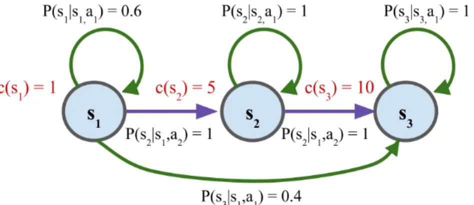
2-1 An example MDP . . . 33

3-1 A graph vs. an occluded graph for the same environment . . . 43

3-2 A graph vs. an occluded graph for the same environment . . . 44

3-3 Transforming an occluded graph into a SSP problem . . . 46

3-4 Resolution completeness for a path with narrowest passageway width 𝑊 48 3-5 An infeasible edge can be due to a variety of configurations of 𝒞𝑜𝑏𝑠 . 49 3-6 Probability distribution for the narrowest passageway in the environ-ment underlying an infeasible edge . . . 50

4-1 CEIMP works with an underlying anytime motion planner . . . 53

4-2 High-level block diagram of CEIMP . . . 55

4-3 High-level block diagram of decision-making . . . 55 5-1 Expected-A* vs. Value Iteration: Difference in Results and Runtime 73

6-1 MIT building floor plans for evaluation . . . 76

6-2 PRM* vs quad-tree . . . 77

6-3 Single trial on Building 13 floor plan on Cortex-A15 . . . 79

6-4 Single trial on Building 31 floor plan on Cortex-A7 . . . 79

6-5 Average results compared to baseline (𝑛𝑚𝑎𝑥 = 20, 000) on MIT floor plans . . . 80

6-6 Varying difficulty of finding a homotopic class with a shorter path and savings when finding that class . . . 81

6-7 Total energy for CEIMP and baseline across a range of simulated values of the cost-of-computing and the cost-of-transport . . . 83

6-8 Effect of baseline 𝑛𝑚𝑎𝑥 on CEIMP performance . . . 84

List of Tables

1.1 Analogies for motion plan execution and computation tasks . . . 18 3.1 % repaired edges with narrowest passageway width 𝑊 on different floor

plans . . . 51 6.1 Runtime breakdown by function . . . 85

Chapter 1

Introduction

1.1

Overview of Low-Power Robotics

Imagine a world with swarms of miniature palm-size drones assisting in search-and-rescue missions, robotic water striders roaming the oceans to tag plastics, credit-card-sized satellites exploring distant parts of the universe, and medical robots intelligently navigating the human body to treat illnesses in new ways. These types of applications may one day be possible using robots with a small form factor or long duration endurance; however, these qualities also make the robot severely power constrained.

Researchers have shown increasing interest in developing low-power robotic plat-forms with a small form factor or a long deployment duration, as seen by examples in Figure 1-1. Insect-scaled flapping-winged robots have shown recent successes in research labs such as the Robobee which requires 26-35 milliWatts (mW) of actua-tion power for untethered flight, and the Robofly which requires 50 mW of actuaactua-tion power during a hovering maneuver [1, 2]. Insect-scaled robotic water striders have shown to be able to move on and jump off water surfaces using 13.5 mW of power [3]. Robots do not need to be only insect-sized to consume extremely low-power for actu-ation. Researchers have developed autonomous lighter-than-air vehicles in the form of a miniature autonomous blimp; in one case, the blimp can operate up to 400 hours consuming only 200 mW for actuation [4]. In commercial use, the Seaglider is an ocean glider that measures 1.8 meters in length, weighs up to 56 kilograms with

pay-Figure 1-1: Examples of low-power platforms [1, 2, 3, 4, 5, 6, 7, 8]

load, and has a maximum mission duration of 200 days, all while consuming only 500 mW, leveraging buoyancy to keep the actuation power consumption low [5].

While there exists an active research field into developing low-power actuated robotic platforms, a similar degree of attention has not been paid to how to design low-power autonomy on-board the vehicle. Popular embedded computing platforms include embedded central processing units (CPUs) such as the ARM Cortex-A7 and ARM Cortex-A15, embedded graphic processing units (GPUs) such as the Nvidia Jet-son TX2, field programmable gate arrays (FPGAs), and application specific integrated circuits (ASICs). Figure 1-2 shows various low-power robotic platforms arranged by each platform’s energy to move one meter, calculated by dividing the actuation power 𝑃𝑎 in Joules per second (J/s) by the vehicle speed 𝑣𝑎 in meters per second (m/s). We

also show various embedded computers arranged by each computer’s energy to com-pute one second, given by the computing power 𝑃𝑐. It is evident that for low-power

robotic vehicles equipped with embedded computing running algorithms for auton-omy, the energy to compute one more second is on a similar magnitude to the energy to move one more meter.

Consider, for example, the Cheerwing mini RC car [8]; with an actuation power approximately equal to 4.9 Watts (W) at 5.4 m/s vehicle speed, the car has an energy per meter equal to 0.91 J/m. With an embedded CPU consuming on average one Watt, computing another one second is as expensive as moving another 1.1 meters.

Figure 1-2: Energy to move one meter vs. energy to compute one more second on low-power robotic platforms and embedded computers [1, 5, 9]

With an embedded GPU Nvidia Jetson TX2 consuming on average 7.5 W, computing another one second is as expensive as moving another 8.25 meters. In the 3D case, the Viper Dash [7] can fly at speeds up to approximate 11.2 m/s at 5.5 W, making its energy per meter equal to 0.49 J/m. With a computer averaging one Watt of power consumption, computing another one second is as expensive as moving 2.05 meters. When the Viper is equipped with a computer that consumes 7.5 W, computing for one second is as expensive as moving another 15.3 meters!

1.2

Total Energy of Motion Planning

In this thesis, we address this new class of problems where the energy a robot spends for actuation during its motion is comparable to the energy spent computing the path. Table 1.1 shows the analogies between these two tasks. For the motion ex-ecution task, a robot must move along a path with length 𝑙𝑎, at a speed 𝑣𝑎, for a

Table 1.1: Analogies for motion plan execution and computation tasks

Actuation Computing

- Num. of nodes [nodes], 𝑛 Path length [m], 𝑙𝑎(𝑛) Num. of operations [ops], 𝑙𝑐(𝑛)

Vehicle speed [m/s], 𝑣𝑎 Processing speed [ops/s], 𝑣𝑐

Actuation power [W], 𝑃𝑎(𝑣𝑎) Computing power [W], 𝑃𝑐(𝑣𝑐)

Actuation time [s], 𝑡𝑎(𝑙𝑎(𝑛), 𝑣𝑎) Computing time [s], 𝑡𝑐(𝑙𝑐(𝑛), 𝑣𝑐)

Actuation energy [J], 𝐸𝑎 Computing Energy [J], 𝐸𝑐

duration of actuation time 𝑡𝑎, drawing motor power 𝑃𝑎, and expending actuation

en-ergy 𝐸𝑎; for the motion-plan computation task, its computer must compute 𝑛 number

of nodes, requiring 𝑙𝑐 computer operations, at a processing speed of 𝑣𝑐, for a

dura-tion of computing time 𝑡𝑐, drawing computing power 𝑃𝑐, and expending computing

energy 𝐸𝑐. We can think of 𝑙𝑐 as the length of the computation, which is analogous

to the length of the path 𝑙𝑎. In a conventional setting where 𝐸𝑐≪ 𝐸𝑎, only the first

energy term for actuation energy in Equation (1.1) is used to evaluate a motion plan-ning algorithm since it dominates the total energy. Planplan-ning algorithms will return monotonically decreasing path lengths with increasing number of nodes computed, meaning to minimize only actuation energy, it is necessary to compute the maximum number of nodes possible. However, when the energy required for computing is not negligible compared to the energy required for actuation, we must consider both the energy of executing and computing a candidate solution:

𝐸𝑡= 𝐸𝑎+ 𝐸𝑐 = 𝑃𝑎(𝑣𝑎)𝑡𝑎(𝑙𝑎(𝑛), 𝑣𝑎) + 𝑃𝑐(𝑣𝑐)𝑡𝑐(𝑙𝑐(𝑛), 𝑣𝑐) = 𝑃𝑎(𝑣𝑎) 𝑣𝑎 𝑙𝑎(𝑛) + 𝑃𝑐(𝑣𝑐) 𝑣𝑐 𝑙𝑐(𝑛). (1.1)

Equation (1.1) can be considered as the “cost-to-move” and the “cost-to-compute”, making up the total energy 𝐸𝑡 when considering actuation and computing energy.

This trade-off is depicted in Fig. 1-3, where we run a sampling-based motion planner on an embedded CPU (ARM Cortex A-15) and present averaged results over 1000 trials on the MIT Building 31 floor plan. We calculate the computing energy by

0 2500 5000 7500 10000 12500 15000 17500 20000 Number of nodes 0 20 40 60 80 100 Energy [J] Total Energy (

E

+ E

Figure 1-3: Computing energy and actuation energy vs. nodes in a sampling-based motion planner, PRM* [10]

using the average computing power of the ARM Cortex A-15 at 2.33 W and the computing time. We calculate the actuation energy by using the path length returned by the planner and assume a robot platform that has an energy per meter equal to one Joule per meter, such that it moves at one meter per second per one Watt spent. If we only look to minimize actuation energy, we end at the purple marker on the total energy curve, far from the minimum of the total energy. Minimizing actuation and computing energy involves stopping computation earlier at the red marker and accepting a larger “cost-to-move” for a lower “cost-to-compute”. While path length 𝑙𝑎(𝑛) explicitly depends on how many nodes 𝑛 the planner computes, the

exact relationship between 𝑙𝑎(𝑛) and 𝑛 is uncertain at any number of nodes less than

𝑛, such that the path length in 𝑛 nodes before computing 𝑛 nodes is uncertain. In other words, the actuation energy is uncertain until we spend the computing energy to compute it, making Equation (1.1) a challenging objective function to minimize.

1.3

Background on Motion Planning

Broadly, the motion planning problem is to find a sequence of states that moves an agent from its starting configuration to its desired goal configuration without colliding

into obstacles in the environment. We call the sequence of states a path 𝜎, and we call a collision-free path a feasible path. Optimal motion planning is finding a feasible path that minimizes an objective function. More formally, let 𝒞 denote the configuration space, which is the set of all values the state of the robot take on, and let 𝒞𝑜𝑏𝑠 denote

the obstacle space, which is the set of all values the state of the robot can take on that is also in collision with an obstacle. Let 𝒞𝑓 𝑟𝑒𝑒 = 𝒞 ∖ 𝒞𝑜𝑏𝑠 denote the free space.

A path 𝜎 is a continuous function in the configuration space, such that 𝜎 : [0, 1] → 𝒞 [11]. Given a start configuration 𝑐𝑠 ∈ 𝒞𝑓 𝑟𝑒𝑒 and a goal configuration 𝑐𝑔 ∈ 𝒞𝑓 𝑟𝑒𝑒, we

aim to find a feasible path 𝜎 : [0, 1] → 𝒞𝑓 𝑟𝑒𝑒, starting in 𝑐𝑠, reaching 𝑐𝑔, avoiding 𝒞𝑜𝑏𝑠,

that minimizes the objective function 𝑓 ,

minimize

𝜎 𝑓 (𝜎)

subject to 𝜎(0) = 𝑐𝑠, 𝜎(1) = 𝑐𝑔, 𝜎 ∈ 𝒞𝑓 𝑟𝑒𝑒.

(1.2)

Typically, the objective function 𝑓 (𝜎) is often the length of path 𝜎 as a representative for actuation energy. In this case, optimal motion planning is equivalent to finding the shortest obstacle-free path from the start to the goal. In this thesis, we will change this objective function to equal 𝐸𝑡, such that optimal motion planning for the new

class of problems is equivalent to finding the obstacle-free path from the start to the goal that minimizes the sum of both actuation energy and computing energy (i.e., total energy, which is indicated by the subscript in 𝐸𝑡).

While solving the motion planning problem is NP-hard in the worst-case, prob-abilistic sampling-based planning algorithms solve the problem in practice for the average case. Sampling-based motion planning algorithms solve the motion plan-ning problem by "probing" or discretizing the configuration space either determin-istically (e.g., grid-based approaches) or stochastically (e.g., random sampling-based approaches) to assemble the set of nodes 𝑁 [11]. Note, we refer to the cardinality of the set 𝑁 by the variable 𝑛. The nodes are connected via the set of edges 𝑀 to form a graph 𝐺 = (𝑁, 𝑀 ) that captures the connectivity of the environment. An edge consists of a paired edge source node 𝑐 and edge destination node 𝑐′ in 𝒞, and

(a) Environment (b) Deterministic discretiza-tion (e.g., grid)

(c) Stochastic discretization (e.g., PRM*)

Figure 1-4: Grid-based motion planning vs. sampling-based motion planning

is denoted as (𝑐, 𝑐′) ∈ 𝑀 . In Figure 1-4, the environment is "probed" or discretized by sampling 36 nodes (gray circles), either deterministically through grid sampling or stochastically through random sampling (e.g., a probabilistic roadmap planner (PRM*) [10]). The nodes are connected via feasible edges (gray lines) and infeasible edges that are in collision with 𝒞𝑜𝑏𝑠 (red lines). Sampling-based motion planners treat

collision checking as a black box that outputs whether a node or edge is in collision with the obstacle space. Typically, only edges that are collision-free are added to the graph [11].

Generally, after sampling nodes and connecting edges, motion planners will run a path search algorithm on the feasible nodes and edges of the graph to find the shortest path, with a notable exception of rapidly-exploring random trees (RRT*), which maintains a tree structure instead of a graph [10]. Path search algorithms find the shortest weighted path between nodes in a graph by traversing the feasible edges of the graph and maintaining a priority queue of partial paths to visit. This problem was originally solved by Dijkstra’s algorithm, which orders partial paths in the priority queue based on the cost so far [12]. A popular variant of Dijkstra is A*, which orders partial paths in the priority queue by the sum of the “cost-to-come” and an optimistic heuristic to estimate of the “cost-to-go” that underestimates the real “cost-to-go” such as the Euclidean distance to the goal [13]. With a good heuristic that is close the real “cost-to-go”, A* shows improved performance compared to Dijkstra’s algorithm

by needing to visit fewer nodes to find the shortest path.

In general, a motion planner samples a specified number of nodes, connects the nodes while checking for collisions, and runs a path search algorithm at the end before returning a candidate path. However, for deployment in the real-world where the environment is uncertain and dynamic leading to latency constraints on planning, we desire planners that we can query from "anytime" in case we need a feasible solution quickly even before the maximum number of nodes have been computed. An anytime motion planner quickly finds a feasible path solution that may not be optimal, and incrementally improves upon it over time [14]. For example, a grid-based algorithm can be made into an anytime algorithm by running a path search before discretizing to the next resolution level, and a PRM* can be made into an anytime algorithm by sampling in batches and running a path search between batches.

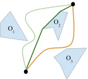
As the planner places more nodes, the path length monotonically decreases. The two sources of the reduction in the path length as we put down more nodes are homotopic class changes and local optimization within a single homotopic class, as illustrated in Figure 1-5. Intuitively, two paths are in the same homotopic class if one path can be "warped" continuously into the other path. This deformation is called homotopy [11]. For example, the light green and dark green paths in Figure 1-5 are within the same homotopic class. However, the orange path is in a different homotopic class since the obstacle between the paths represents a discontinuity such that the orange line cannot be continuously warped into either of the green lines. Reductions in path length can occur from a homotopic class change when further discretization of the state space reveals a new homotopic class that was not seen before. The second source of reduction in path length comes from local optimization within a single homotopic class, where more nodes placed in the configuration space cause the shortest path in the graph to asymptotically approach the true minimum length path in that homotopic class as the number of nodes approach infinity. In Figure 1-5, the dark green path illustrates a locally optimized path in the same homotopic class as the original light green path.

Figure 1-5: Original path (light green) undergoing local optimization in the same homotopic class (dark green) and homotopic class change (orange)

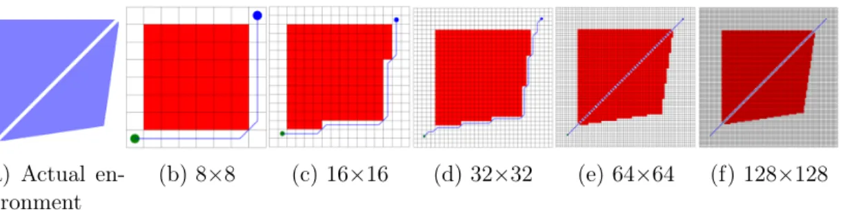
resolution step (64 nodes), the path length decreases with increasing discretization up to the 32×32 grid resolution step (1024 nodes) due to local optimization within the same homotopic class. At the 64×64 grid resolution step (4096 nodes), the path length decreases again, now due to a homotopic class change by finding the narrow passageway shortcut between the obstacles. Doubling the resolution again to get to the 128×128 grid resolution step (16,384 nodes) results in local optimization within the second homotopic class found. While local optimization can be modeled more easily, modeling future homotopic class changes without discretizing further is non-trivial. For example, at the 16×16 grid resolution step, we can model how much we expect the path to reduce from local optimization if we discretize again based only on what we know in the 16×16 grid resolution step. However, at the 32×32 grid resolution step, it is challenging to predict that a new homotopic class will open up in the next round of discretization based on only what we see at the 32×32 grid resolution step. We address a new solution to model future homotopic class changes in this thesis.

(a) Actual en-vironment

(b) 8×8 (c) 16×16 (d) 32×32 (e) 64×64 (f) 128×128

Figure 1-6: Shortest paths in the same environment at different grid resolutions

1.4

Related Work

Efficient Motion Planning

There has been a large body of work looking at heuristics to reduce the “cost-to-compute” term towards efficient motion planning. In particular, variants of RRT* and PRM* [10] were proposed towards reducing the number of operations 𝑙𝑐(𝑛) for a

given 𝑛, which results in a lower 𝐸𝑐. These methods include Batch-Informed Trees

(BIT*) [15], which employs incremental search techniques to reuse previous compu-tation, and Fast Marching Trees (FMT*) [16], which lazily checks if an edge is in collision after first finding the locally-optimal best edge to connect. Other works have also focused on allowing edges in a graph to be in obstacle space to speed up computation by lowering 𝑙𝑐(𝑛). Hsu et al. [17] looked at dilating free space as a

heuris-tic to find paths through narrow passageways to later repair, effectively reducing the number of nodes 𝑛 required on average to find a given path. Bohlin et al. [18] pro-posed Lazy PRM, which searches for paths before doing collision checks to minimize computing on collision checks, lowering 𝑙𝑐(𝑛) for a given 𝑛. While all these works

lower 𝐸𝑐 by lowering 𝑙𝑐(𝑛), they still maintain the goal of finding the paths with the

lowest 𝐸𝑎. They do not consider balancing both 𝑙𝑎(𝑛) and 𝑙𝑐(𝑛) and allowing for

trade-offs between 𝐸𝑎 and 𝐸𝑐. In this respect, the work we present in this thesis is a

more aggressive approach to lowering total energy, where we allow a larger 𝑙𝑎(𝑛) as

part of the trade-off to reduce 𝑙𝑐(𝑛).

In addition to algorithmic efficiency improvements, researchers have studied build-ing specialized hardware to do motion plannbuild-ing computation more efficiently to lower

𝐸𝑐. Murray et al. [19] used an FPGA to speed up motion planning for an armed

manipulator by exploiting the parallelism of collision checking. By implementing many parallel collision checking engines, this work effectively reduces computing time 𝑡𝑐(𝑙𝑐(𝑛), 𝑣𝑐) for the motion planning task. Palossi et al. [20] implemented parallelized

planning algorithms on a FPGA to lower 𝑡𝑐(𝑙𝑐(𝑛), 𝑣𝑐) and 𝑃𝑐(𝑣𝑐) for deployment on

a miniature UAV. Unlike these works, we do not focus on optimizing hardware to be highly efficient for a fixed algorithm. Rather, we change the algorithm itself to balance contributions to total system energy 𝐸𝑡 from both actuation hardware and

computing hardware. To the best of our knowledge, the work presented in this thesis is the first work to examine this trade-off between the “cost-to-compute” from the computing hardware and the “cost-to-move” from the actuation hardware to reduce total energy for the motion planning problem.

Multi-Objective Motion Planning

Several works have looked at including contributions to actuation energy other than just path length such as wind and terrain [21, 22]. Ware et al. [21] considered the problem of finding minimum 𝐸𝑎 trajectories in a wind field generated in an urban

environment. Ganganath et al. [22] examined how steepness of an incline can affect 𝐸𝑎

and developed a heuristic to estimate lowest 𝐸𝑎 paths that take terrain into account.

Both of these methods incorporate more dependencies into 𝐸𝑎in addition to 𝑙𝑎(𝑛), and

allow 𝑃𝑎 and 𝑣𝑎 to change realistically based on environmental conditions. However,

while these works add the effect of different environmental variables to the actuation energy, they do not affect the computing energy term of the planning computation task itself.

A large body of work also looks at adding communication costs to the motion planning problem. For example, Yan et al. considers jointly optimizing both com-munication energy and actuation energy, which results in trade-offs between a longer path length, resulting in higher 𝐸𝑎, and a richer connection area, resulting in lower

communication energy cost. Similar to our research, this work adds an additional term to total energy and formulates a trade-off between these terms. However, we

add the computing energy term 𝐸𝑐to total energy 𝐸𝑡, which means we also are trying

to minimize the overhead our solution introduces since the overhead is part of the ob-jective function. This challenge is not present when looking at adding communication energy to the total energy equation.

Scalable Motion Planning Given Computational Constraints

There has also been work on adapting motion planning algorithms given on-board memory and computing time constraints. Larsson et al. [23] use an information the-oretic approach to expose a dial for the resolution of a probabilistic map given a computational power constraint. Their approach examines the trade-off between a lower resolution which corresponds to lower computing power and memory require-ments, and a longer path length in a map where there is uncertainty in whether a cell is occupied. This work involves computing-aware planning and is in the spirit of the work presented in this thesis. However, this work neither considers the computing energy required to plan a path, nor the computing energy required to find the best resolution for the map given computational constraints, to be part of the cost function itself when planning a path. We endeavor to design a decision making scheme that decides online, based on information during planning, when to stop to minimize both actuation and computing energy.

1.5

Thesis Contributions

The contributions of this thesis are as follows:

1. A novel problem formulation for a new class of motion planning problems where the energy to move is comparable to the energy to compute. Here, the cost function to minimize is not only the actuation energy spent to traverse the path, but also the computing energy spent to find that path during planning. We use a dynamic programming framework to turn the problem into an early stopping problem, as illustrated in red in Figure 1-7. We discuss this problem formulation in Chapter 2.

Figure 1-7: Roadmap for Computing Energy Included Motion Planning (CEIMP): CEIMP (green) consists of a decision-making algorithm (red) that requires estimates of expected future 𝐸𝑐 and 𝐸𝑎 (purple). 𝐸𝑐 and 𝐸𝑎 will change as we increase 𝑛 due

to the processes of motion planning (blue), and we introduce efficient ways to model those processes (yellow).

2. In order to solve the stopping problem, we must have an estimate on expected future computing energy costs and expected future actuation energy savings, as illustrated in purple in Figure 1-7. While predicting future computing energy costs and actuation energy savings from local optimization can be easily mod-eled, predicting future actuation energy savings from homotopic class changes is one of the main challenges in this work. We propose a new probabilistic method shown in Figure 1-7 based on constructing an occluded graph to "probe" for new, hard-to-reach homotopic classes, estimating the probability the edges in the occluded graph represent a real homotopic class using Bayesian inference, and approximately solving the stochastic shortest path problem to predict the expected actuation energy change due to homotopic class change. We explain how we model the homotopic class change problem in Chapter 3, and we present the algorithm in Chapter 4.

3. We require an efficient algorithm to decide when to stop computing since the overhead computing energy we spend on decision-making is part of the total

energy cost function we want to minimize. In order to efficiently estimate the value of continuing to plan, we introduce an approximation to solve the stochastic shortest path problem in motion planning called Expected-A* with two orders of magnitude less overhead than value iteration. We describe the Expected-A* algorithm in detail in Chapter 4 and discuss error bounds on its performance in Chapter 5.

4. A new algorithm called Computing Energy Included Motion Planning (CEIMP) that selects when to stop computing to minimize total energy for any anytime sampling-based motion-planner. CEIMP consists of all the components in Fig-ure 1-7, and solves the stopping problem via backward recursion, using its pre-dictions of future computing energy costs and future actuation energy savings to estimate the value of continuing to compute. The algorithm is discussed in detail in Chapter 4. Analysis of the complexity of the algorithm is discussed in Chapter 5. Results and discussion on computational experiments evaluating the performance of CEIMP is presented in Chapter 6.

A subset of the work presented in this thesis will be published in ICRA 2020 (S. Sudhakar, S. Karaman, V. Sze, “Balancing Actuation and Computing Energy in Mo-tion Planning,” IEEE InternaMo-tional Conference on Robotics and AutomaMo-tion (ICRA), May 2020.).

Chapter 2

Modeling the Low-Power Motion

Planning Problem as an MDP

In this chapter, we model motion planning as a sequential decision-making problem under uncertainty for the class of problems where the actuation energy spent is on a similar magnitude as the computing energy spent. This formulation gives us a method to be able to balance both 𝐸𝑎 and 𝐸𝑐 by evaluating the value of spending

more computing energy to reduce actuation energy.

2.1

Minimizing Total Energy in Motion Planning as

a Stopping Problem

For the new class of motion planning problems where computing energy is no longer negligible, we introduced a new objective function to minimize for optimal motion planning in Chapter 1, 𝐸𝑡= 𝐸𝑎+ 𝐸𝑐 = 𝑃𝑎(𝑣𝑎)𝑡𝑎(𝑙𝑎(𝑛), 𝑣𝑎) + 𝑃𝑐(𝑣𝑐)𝑡𝑐(𝑙𝑐(𝑛), 𝑣𝑐) = 𝑃𝑎(𝑣𝑎) 𝑣𝑎 𝑙𝑎(𝑛) + 𝑃𝑐(𝑣𝑐) 𝑣𝑐 𝑙𝑐(𝑛). (2.1)

In order to reduce the first term in Equation (2.1), which is the actuation energy, we can either switch to a more efficient vehicle with a lower cost-of-transport or we can reduce the amount of mechanical work to complete. The cost-of-transport is the energy required to move one meter, calculated by dividing the actuation power 𝑃𝑎

in Joules per second by the vehicle speed 𝑣𝑎 in meters per second. A more efficient

cost-of-transport can be achieved by designing a vehicle that can go at a faster speed 𝑣𝑎 at the same actuation power 𝑃𝑎, or the same 𝑣𝑎 at a lower 𝑃𝑎. Alternatively, a

reduction in the amount of mechanical work to complete is possible by reducing the length of the path 𝑙𝑎(𝑛) to traverse. In this thesis, we will assume a fixed vehicle

with a fixed cost-of-transport, such that 𝑃𝑎 and 𝑣𝑎 are constant. We will drop the

function notation for these variables for the remainder of the thesis. Thus, only the path length affects the actuation energy term.

Likewise, in order to reduce the second term in Equation (2.1), which is the computing energy, we can either switch to a more efficient computer with a higher cost-of-computing or we can reduce the amount of electrical work to complete. The cost-of-computing is the energy required to compute one operation, calculated by dividing the computing power 𝑃𝑐 in Joules per second by the processing speed 𝑣𝑐

in operations per second. A more efficient cost-of-computing can be achieved by designing a computer that can compute more operations per second 𝑣𝑐 at the same

computing power 𝑃𝑐, or the same 𝑣𝑐 at a lower 𝑃𝑐. Alternatively, we can reduce

the amount of electrical work to complete by lowering the number of operations to compute 𝑙𝑐(𝑛), such as by reducing the number of nodes 𝑛 computed or switching to a

simpler algorithm. In this thesis, we will assume a fixed computer with a fixed cost-of-computing, such that 𝑃𝑐 and 𝑣𝑐 are constant. We will drop the function notation for

these variables for the remainder of the thesis. Thus, only the number of operations affects the computing energy term.

Furthermore, we will consider the option where we lower the number of operations for the computer by lowering the number of nodes computed in the motion planning

algorithm. The objective function to minimize is now, 𝐸𝑡 = 𝑃𝑎 𝑣𝑎 𝑙𝑎(𝑛) + 𝑃𝑐 𝑣𝑐 𝑙𝑐(𝑛) = 𝑃𝑎 𝑣𝑎 𝑙𝑎(𝑛) + 𝑃𝑐𝑡𝑐(𝑙𝑐(𝑛)), (2.2)

where we have dropped dependencies on all variables assumed fixed. Here, the only variable we can change to affect actuation energy and computing energy is the number of nodes 𝑛 computed by the planner, such that we allow the motion planner to stop sampling at 𝑛 ≤ 𝑛𝑚𝑎𝑥nodes instead of 𝑛 = 𝑛𝑚𝑎𝑥 where 𝑛𝑚𝑎𝑥 is the maximum number

of nodes.

As explained in Chapter 1, the relationship between the number of nodes and actuation energy, and the relationship between the number of nodes and computing energy are the opposite from each other, such that for actuation energy, fewer nodes computed results in a higher actuation energy while for computing energy, fewer nodes computed results in a lower computing energy. Moreover, how exactly actuation energy decreases with increasing number of nodes is uncertain until we compute it. Hence, we will introduce a decision-making algorithm to decide how to balance between these two terms. However, spending computing resources to decide whether to devote more computing resources to planning adds a number of operations as overhead that do not contribute to lowering 𝑙𝑎(𝑛), which complicates the problem

even further. With any algorithm estimating the optimal 𝑛*, the total number of operations is equal to 𝑙𝑐(𝑛) = 𝑙𝑐(𝑛) + 𝑙𝑐(𝑛), where 𝑙𝑐 is the number of operations used

in the anytime motion planner to decrease 𝑙𝑎(𝑛) and 𝑙𝑐(𝑛) is the number of operations

used in CEIMP to estimate when to stop computing to lower 𝑙𝑐. To gain savings, it is

necessary to predict 𝑛* to lower 𝑙𝑐 without introducing so much overhead to increase

𝑙𝑐(𝑛) as to negate any energy savings in 𝑙𝑐.

Instead of working with the number of operations 𝑙𝑐(𝑛), we can instead look at

computing time 𝑡𝑐(𝑙𝑐(𝑛)) to avoid having to set the processing speed 𝑣𝑐. The objective

function presented in the second equality in Equation (2.2) shows that the low-power motion planning problem has turned into an early stopping problem to find the

op-timal number of nodes, 𝑛*, to compute that minimizes the sum of actuation and computing energy.

To be noted, the expression for computing energy 𝐸𝑐in Equation (2.1) is a

simpli-fied model for computing energy. In reality, computing energy does not only depend on the computing power, clock speed, and number of operations, but also the types of operations, the bit precision of those operations, and the memory accesses at different levels of the memory hierarchy required to process the workload. These properties are specific to the computer architecture design for each computer. Likewise, a common metric for performance-per-Watt, which is the inverse of cost-of-computing, is the number of floating-point operations per second (FLOPS) per Watt. However, this metric alone is not descriptive enough to evaluate the efficiency of the computing hardware; for example, a computer processor with only multipliers and no memory on chip could have a very high number of FLOPS per Watt for the processor alone, but the entire system could consume much higher power due to the off-chip memory accesses [24]. Having a complete model of the performance of a computer is specific to each computer architecture, and so, we use the simplified expression in Equation (2.1) and Equation (2.2) to represent computing energy.

2.2

Markov Decision Processes and Dynamic

Pro-gramming

To solve the stopping problem to minimize Equation (2.2), we set up the problem as a Markov Decision Process (MDP). An MDP is a stochastic control process that can represent sequential decision-making problem in a stochastic environment; an example MDP is shown in Figure 2-1. It is defined by the following elements:

1. A set of states 𝑆. In the example in Figure 2-1, the set of states are 𝑆 = {𝑠1, 𝑠2, 𝑠3}.

2. A set of actions 𝐴 where each state has associated actions an agent can take to get to other states. In the example in Figure 2-1, the set of actions are

Figure 2-1: An example MDP

𝐴 = {𝑎, 𝑎}, with 𝑎 marked in green and 𝑎 marked in purple.

3. A transition model P(𝑠𝑘+1|𝑎𝑘, 𝑠𝑘) that describes the probability of transitioning

from state 𝑠𝑘 at step 𝑘 to state 𝑠𝑘+1 in the next step 𝑘 + 1 after taking action

𝑎𝑘 at time 𝑘. In the example in Figure 2-1, the transition probability of staying

in state 𝑠1 after taking action 𝑎 to stay is 0.6; with probability equal to 0.4,

the agent instead transitions to state 𝑠3 by taking action 𝑎. The transition

probability for all other state-action pairs is equal to one, such that all other transitions are deterministic.

4. A set of costs (or rewards) for each state. In the example in Figure 2-1, the costs for each state are given in red.

MDPs also exhibit the Markov property, where the conditional probability of future states is only dependent on the current state the agent is in, and not on the previous history of states. In addition, MDPs can be have a finite-horizon or an infinite-horizon. A finite-horizon MDP is a process where there are a finite number of time steps the agent can take before the process ends, while in an infinite-horizon MDP, the process never ends. For the infinite-horizon setting, a discount factor 𝛾 is often introduced to discount future costs or rewards [25].

The MDP framework provides a formalization for sequential decision making un-der uncertainty. For example, in the MDP in Figure 2-1, an agent starting at state 𝑠1

possibly transitioning to the highest cost state 𝑠3, or choose to move to the higher

cost state 𝑠2 where the agent can deterministically choose to stay at state 𝑠2 forever

and never have to transition to highest cost state 𝑠3. Formulating the problem as an

MDP allows us to use dynamic programming techniques to make this decision; we will describe one such technique in Section 2.3.1.

2.2.1

Modeling Low-Power Motion Planning as an MDP

In order to make a decision on the number of nodes 𝑛 to stop computing at to minimize Equation (2.2), we will formulate the problem as a continuous state-space finite-horizon MDP. Our problem set-up is as follows: to plan a path from the desired start to the goal, the anytime motion planner (e.g., PRM*) samples a batch of nodes in the configuration space. Between each batch of nodes, the anytime planner searches for the current best feasible path. At this point, we solve a dynamic programming problem to decide whether to continue computing to find a shorter feasible path or to stop computing and accept the current best feasible path. We set a maximum number of nodes 𝑛𝑚𝑎𝑥, and therefore, a maximum number of batches 𝑘𝑚𝑎𝑥, such that

if we decide to continue for the first 𝑘𝑚𝑎𝑥− 1 batches, we have to stop computing and

return the best feasible path after the last batch of nodes.

More formally, let the number of nodes in the batch equal 𝑏, such that after the 𝑘𝑡ℎ batch, the planner has computed 𝑛 = 𝑏𝑘 number of nodes. Let 𝑐𝑠 be the start

node, 𝑐𝑔 be the goal node, 𝑎 be the action to continue computing, 𝑎 be the action to

stop computing, 𝑠𝑘 be the state after the 𝑘𝑡ℎ batch, 𝑎𝑘 be the action taken after the

𝑘𝑡ℎ _{batch, and 𝑔}

𝑘(𝑠𝑘, 𝑎𝑘) be the cost incurred at state 𝑠𝑘 taking action 𝑎𝑘 after the

𝑘𝑡ℎ batch. We define the state 𝑠𝑘 as a vector made up of the path length after the 𝑘𝑡ℎ

batch, 𝑙𝑎(𝑏𝑘), and the computing time the planner spent on the previous 𝑘𝑡ℎ batch,

(𝑗 − 𝑘) batches as ∆𝑡𝑐(𝑙𝑐(𝑏𝑗)) = 𝑡𝑐(𝑙𝑐(𝑏𝑗)) − 𝑡𝑐(𝑙𝑐(𝑏𝑘)). Then, States: 𝑙𝑎(𝑏𝑘) ∈ [||𝑐𝑠− 𝑐𝑔||2, 𝑙𝑎(𝑏(𝑘 − 1))] ∆𝑡𝑐(𝑙𝑐(𝑏𝑘)) ∈ [0, ∞) Actions: 𝑎𝑘 ∈ ⎧ ⎪ ⎨ ⎪ ⎩ {𝑎, 𝑎} if 𝑎𝑘−1 = 𝑎 {𝑎} if 𝑎𝑘−1 = 𝑎

Transition function: P(𝑠𝑘+1|𝑎𝑘, 𝑠𝑘) for all 𝑠 ∈ 𝑆

Per-batch cost: 𝑔𝑘(𝑠𝑘, 𝑎𝑘) = ⎧ ⎪ ⎪ ⎪ ⎪ ⎪ ⎨ ⎪ ⎪ ⎪ ⎪ ⎪ ⎩ 𝑃𝑐∆𝑡𝑐(𝑙𝑐(𝑏𝑗)) if 𝑎𝑘= 𝑎 (𝑃𝑎/𝑣𝑎)𝑙𝑎(𝑏𝑘) if 𝑎𝑘= 𝑎 0 if 𝑎𝑘−1 = 𝑎 Total cost: 𝐸𝑡= 𝐾 ∑︁ 𝑘=1 𝑔𝑘(𝑠𝑘, 𝑎𝑘).

In this formulation, once action 𝑎 is chosen to stop, the process ends so that the agent incurs no additional costs for future batches it chooses to not compute. In an MDP for a stopping problem, we model the state after stopping as an absorbing state, such that the agent’s only action from this state is 𝑎 (stopping again) with no reward; in practice, we simply stop simulating the process once the decision is made to stop computing. Note, the cumulative total cost 𝐸𝑡 is the same as the total energy term,

𝐸𝑡 = 𝐸𝑎+ 𝐸𝑐, in Equation (2.2). Furthermore, the state 𝑙𝑎(𝑏𝑘) is bounded below by

the Euclidean distance path from the start node to the goal node and bounded above by the best feasible path found after the previous batch 𝑙𝑎(𝑏(𝑘 − 1)) since motion

planning returns path lengths that are monotonically decreasing.

The transition function, P(𝑠𝑘+1|𝑎𝑘, 𝑠𝑘) for all 𝑠 ∈ 𝑆, is unknown, and finding an

estimate for the transition function is one of the main tasks we must solve to be able to reduce total energy. We cover how we model the MDP approximately in Section 2.3.2 and how we estimate the transition function in Chapters 3 and 4.

2.3

The Value of Continuing to Compute

In our problem formulation, after every batch of samples, we must decide whether it is worth it to continue sampling more nodes or whether the path we have already found is good enough. How do we formalize "worth it" and "good enough" in the MDP setting?

The quantity of interest is the expected cost the agent will incur over the process given its current state if it follows a policy 𝜋, which is a sequence of actions made up of the actions the agent will take at each batch. In our case, once we stop, we cannot continue again, so the policy 𝜋 always transitions from 𝑎 to 𝑎 after some number of batches, where 𝜋 = [𝑎, ..., 𝑎,𝑎, ..., 𝑎]. We wish to find the best batch to transition from 𝑎 to 𝑎, which can range from stopping immediately to continuing to 𝑛𝑚𝑎𝑥 nodes

to stopping in any batch in between. The expected cost the agent will incur over the process given its current state if it follows 𝜋 is called the value function and can be defined recursively by,

𝑉𝜋(𝑠𝑘) = E [︃_{𝑘𝑚𝑎𝑥−1} ∑︁ 𝑗=𝑘 (𝑔𝑗(𝑠𝑗, 𝑎𝑗)) + 𝑔𝑘𝑚𝑎𝑥(𝑠𝑘𝑚𝑎𝑥)|𝜋 ]︃ = E𝑠𝑘+1∈𝑆[𝑔𝑘(𝑠𝑘, 𝑎𝑘) + 𝑉 𝜋 (𝑠𝑘+1)] . (2.3)

The optimal value function 𝑉*(𝑠𝑘) is the lowest expected cost the agent will incur

over the process by taking the optimal policy 𝜋* which is the sequence of actions that minimize the total cost for the agent, described by,

𝑉*(𝑠𝑘) = min𝑎𝑘∈𝐴{E𝑠𝑘+1∈𝑆[𝑔𝑘+ 𝑉 * (𝑠𝑘+1)]} , (2.4) and, 𝜋*(𝑠) = argmin_𝑎 𝑘∈𝐴{E𝑠𝑘+1∈𝑆[𝑔𝑘(𝑠𝑘, 𝑎𝑘) + 𝑉 *_(𝑠 𝑘+1)]} . (2.5)

take the action that minimizes the expected total cost: 𝑉*(𝑠𝑘) = min {︂ 𝑃_𝑎 𝑣𝑎 𝑙𝑎(𝑏𝑘), E [𝑃𝑐∆𝑡𝑐(𝑙𝑐(𝑏𝑗)) + 𝑉*(𝑠𝑘+1)] }︂ . (2.6)

The first term in Equation (2.6) is the value function of stopping at state 𝑠𝑘, and is

simply the actuation energy with the path length found after 𝑘 batches. The second term is the value of continuing to compute and consists of the sum of the computing energy for another batch and the value function of the next state.

2.3.1

Backward Recursion for Finite-Horizon MDPs

We can solve for the optimal value function and policy by using the dynamic pro-gramming algorithm, shown in Algorithm 1 [26]. The main insight of the algo-rithm is that since optimal paths are made up of optimal sub-paths, we can ap-ply backward recursion where we start from a known terminal value function and step backward to find 𝜋*. If we are to apply the dynamic programming problem to our stopping problem, we will need to calculate 𝑉*(𝑠𝑗) for future batches 𝑗, where

𝑗 = 𝑘 + 1, 𝑘 + 2, ..., 𝑘. To calculate 𝑉*(𝑠𝑗), we need the transition model for the path

length 𝑙𝑎(𝑏𝑗) and the transition model for the computing energy for (𝑗 − 𝑘) batches.

Algorithm 1: Dynamic Programming Algorithm

1 𝑉*(𝑠_{𝑘𝑚𝑎𝑥}) = 𝑔_{𝑘𝑚𝑎𝑥}(𝑠_{𝑘𝑚𝑎𝑥}, 𝑎_{𝑘𝑚𝑎𝑥});

2 for 𝑗 = 𝑘𝑚𝑎𝑥− 1, ..., 𝑘 do

3 𝑉*(𝑠𝑗) = min𝑎𝑗∈𝐴(𝑠𝑗){E[𝑔𝑗(𝑠𝑗, 𝑎𝑗) + 𝑉

*_(𝑠 𝑗+1)]};

2.3.2

Approximate Dynamic Programming

Calculating 𝑉*(𝑠𝑗) exactly can be very computationally expensive, since we do not

have the transition model for the path length 𝑙𝑎(𝑏𝑗) and the transition model for the

computing energy ∆𝑡𝑐(𝑙𝑐(𝑏𝑗)) in the next (𝑗 − 𝑘) batches. Instead, we will introduce

approximation in value space to efficiently approximate the optimal value function 𝑉*(𝑠𝑗) with ̃︀𝑉 (𝑠𝑗). The problem is now an example of approximate dynamic

estimated. Instead of minimizing Equation (2.4), we now minimize, min𝑎𝑘∈𝐴 {︁ E𝑠𝑘+1∈𝑆[𝑔𝑘+ ̃︀𝑉 (𝑠𝑘+1)] }︁ , (2.7)

where our estimated ̃︀𝑉 (𝑠𝑘+1) has replaced the optimal 𝑉*(𝑠𝑘+1). Approximation

in value space results in sub-optimal policies, but is necessary here to make the problem tractable [26]. In order to calculate ̃︀𝑉 (𝑠𝑗), we will need to estimate the

future expected path length E[𝑙𝑎(𝑏𝑗)] ≈ E[̃︀𝑙𝑎(𝑏𝑗)] at batch 𝑗, and future computing

energy ∆𝑡𝑐(𝑙𝑐(𝑏𝑗)) ≈ ̃︂∆𝑡𝑐(𝑙𝑐(𝑏𝑗)) to model computing energy for batch 𝑗. These

estimates allows us to calculate an approximated cost_̃︀𝑔𝑗(𝑠𝑗, 𝑎𝑗) for batch 𝑗, and solve

the approximate dynamic program using Algorithm 2.

Algorithm 2: Approximate Dynamic Programming Algorithm

1 𝑉 (𝑠̃︀ _{𝑘𝑚𝑎𝑥}) = E[̃︀𝑔_{𝑘𝑚𝑎𝑥}(𝑠_{𝑘𝑚𝑎𝑥}, 𝑎_{𝑘𝑚𝑎𝑥})]; 2 for 𝑗 = 𝑘𝑚𝑎𝑥− 1, ..., 𝑘 do 3 𝑉 (𝑠̃︀ _𝑗) = min_𝑎 𝑗∈𝐴(𝑠𝑗) {︁ E[̃︀𝑔𝑗(𝑠𝑗, 𝑎𝑗) + ̃︀𝑉 (𝑠𝑗+1)] }︁ ;

Note, since we cannot calculate the optimal policy 𝑉*(𝑠𝑘) and instead are

calcu-lating a sub-optimal policy, we will re-solve Algorithm 2 after each batch of nodes is computed in an online fashion. Based on how the approximation in value space is calculated, this adaptive approach can result in better policies as the number of batches increases since a sub-optimal policy calculated once at the beginning of the problem has less information to approximate ̃︀𝑉 (𝑠𝑗) accurately.

2.4

Summary

In this chapter, we modeled how to minimize the total energy in motion planning by allowing a planner to stop planning earlier than at the maximum number of nodes. The MDP formulation of this stopping problem allows us to formalize how to decide when to stop based on the current value of stopping and the expected value of contin-uing to compute. However, calculating the expected value of contincontin-uing to compute is non-trivial, since we do not have a transition model for how the path length will

evolve with the more nodes the planner computes. A reduction in path length can occur from either changes in homotopic class or local optimization within a single homotopic class. We will discuss foundations on how to model future savings in path length from changes in homotopic class next in Chapter 3, and we will discuss how we can model local optimization of a path and the future cost of computing itself in Chapter 4. Putting together all the elements in Chapter 4 gives us an algorithm to solve the MDP we have set up in this chapter, and therefore, reduce total energy of motion planning.

Chapter 3

Modeling Homotopic Class Changes

in Motion Planning

As discussed in Chapter 1, further computation can reduce the path length due to either local optimization within a single homotopic class or due to homotopic class change of the shortest path. Local optimization within a single homotopic class can easily be modeled using a dispersion model, and we discuss the specific model we use in Chapter 4. On the other hand, modeling homotopic class changes is non-trivial, and we discuss foundations for how to approach this modeling problem in this chapter.

3.1

Challenges in Predicting Homotopic Class Change

Unlike local optimization within a single homotopic class, path length reduction due to a homotopic class change depends on whether a new sample is able to connect a shorter feasible path through a previously unconnected homotopic class. An exact method to predict which homotopic class will open up in the future requires enu-merating all homotopic classes within an environment, identifying which class our current shortest path is within, and having a transition model for sampling con-nectivity within each homotopic class given more samples. However, enumerating all the possible homotopic classes is exponential in the number of obstacles in the environment [27], and thus an exact model would require much more overhead

oper-ations 𝑙𝑎(𝑛) than savings in the planner’s operations 𝑙𝑎(𝑛). Moreover, we desire an

algorithm that does not scale in complexity with the number of obstacles, much like sampling-based motion planners.

Instead of an exact method, we next introduce a novel method to model path length savings from homotopic class changes. In this method, we explore obstacle space to identify potential homotopic classes, and estimate how likely we are to find a path through these potential homotopic classes in order to calculate the expected shortest path length after further computation.

3.2

Exploring Obstacle Space

We take inspiration from sampling-based motion planners. Instead of explicitly con-structing the obstacle space 𝒞𝑜𝑏𝑠, sampling-based motion planners "probe" or sample

the configuration space 𝒞, use a black-box collision detector to discard nodes and edges in 𝒞𝑜𝑏𝑠, and search for the shortest path in 𝒞𝑓 𝑟𝑒𝑒 [11]. Similarly, instead of

ex-plicitly constructing the set of all homotopic classes, we will use a method that probes 𝒞 by sampling nodes and connecting edges. However, instead of discarding edges that are found to be in 𝒞𝑜𝑏𝑠, we will keep track of those edges and estimate whether these

edges are close to a new homotopic class that contains a path in 𝒞𝑓 𝑟𝑒𝑒.

We begin by defining the state of an edge, the process of repairs, and an occluded graph.

Definition 1 (real and unreal edge states). The state of an edge (𝑐, 𝑐′) is the Bernoulli variable 𝑋(𝑐,𝑐′₎ that takes on two values, real (𝑥) or unreal (𝑥), with

prob-ability P(𝑋(𝑐,𝑐′₎ = 𝑥). We denote the estimate of P(𝑋_(𝑐,𝑐′₎ = 𝑥) at the 𝑘𝑡ℎ batch as

𝑝(𝑐,𝑐′₎(𝑘). A real edge is a currently infeasible edge in 𝒞_𝑜𝑏𝑠 that can be repaired by

future sampling. An unreal edge is a currently infeasible edge that cannot be repaired by future sampling.

Definition 2 (repairing). We can repair an infeasible edge (𝑐, 𝑐′) by sampling in a ball centered on the midpoint of of the segment connected by (𝑐, 𝑐′) with diameter

(a) 𝐺 = (𝑁, 𝑀 ) (b) 𝐺_{𝑜𝑐𝑐𝑙} = (𝑁, 𝑀, 𝑃 )

Figure 3-1: A graph vs. an occluded graph for the same environment

𝛼||𝑐 − 𝑐′||2 and finding a path 𝜎 ∈ 𝒞𝑓 𝑟𝑒𝑒 from 𝑐 to 𝑐′. If such a path is found, the

infeasible edge is repaired (𝑟). If such a path is not found, the infeasible edge is unrepaired (𝑟). We set 𝛼 as a parameter that relates how much of an increase in path length we allow a repair to make.

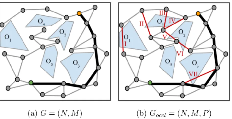
Definition 3 (occluded graph). An occluded graph 𝐺𝑜𝑐𝑐𝑙 = (𝑁, 𝑀, 𝑃 ) is a graph

made up of the set of nodes 𝑁 ∈ 𝒞𝑓 𝑟𝑒𝑒, set of edges 𝑀 ∈ (𝒞𝑓 𝑟𝑒𝑒∪ 𝒞𝑜𝑏𝑠), and a set of

probabilities 𝑃 : 𝑝(𝑐,𝑐′₎(𝑘) ∀(𝑐, 𝑐′) ∈ 𝑀 that maps each edge to the probability of the

edge being a real edge.

Figure 3-1 shows an example of a graph 𝐺 and an occluded graph 𝐺𝑜𝑐𝑐𝑙, where

feasible edges are marked in gray, infeasible edges are marked in red, and the current shortest feasible path is marked in black. The infeasible edges I and III are examples of unreal edges, while the remaining infeasible edges are examples of real edges. We see an example of real and unreal edges in practice on a PRM* on an MIT Building 31 floor plan in Figure 3-2. For instance, the edges circled in yellow in Figure 3-2 narrowly miss making a collision-free connection across a narrow passageway and are real edges, since the planner can likely repair the edges with more sampling. On the other hand, the other infeasible edges that cross walls cannot be repaired with any amount of sampling, and are unreal. While not marked on the figures, note each infeasible edge in Figures 3-1 and 3-2 has an associated probability of being a real edge, 𝑝(𝑐,𝑐′₎(𝑘) at the 𝑘𝑡ℎ batch. We discuss different ways to estimate 𝑝_(𝑐,𝑐′₎(𝑘) for

(a) An occluded graph PRM* on a real floor plan

(b) A close-up on real and unreal edges

Figure 3-2: A graph vs. an occluded graph for the same environment

each infeasible edge in Section 3.4 and Section 4.5.2.

The concept of repairing a current infeasible edge necessitates "freezing" 𝐺𝑜𝑐𝑐𝑙

after a threshold of 𝜂 nodes, such that nodes added to the anytime planner’s graph 𝐺 for the underlying motion planning algorithm after 𝜂 nodes are not added to 𝐺𝑜𝑐𝑐𝑙.

Instead, these new samples are used to infer whether the existing infeasible edges are real or unreal by updating 𝑝(𝑐,𝑐′₎(𝑘) for each infeasible edge in 𝐺_{𝑜𝑐𝑐𝑙}. We refer to

the event that we repair edge (𝑐, 𝑐′) at (𝑗 − 𝑘) batches from the current batch, 𝑘, as 𝑌(𝑐,𝑐′₎(𝑗 − 𝑘), and the probability that we repair edge (𝑐, 𝑐′) at (𝑗 − 𝑘) batches from

the current batch, 𝑘, as P(𝑌(𝑐,𝑐′₎(𝑗 − 𝑘)) for 𝑗 = 𝑘 + 1, 𝑘 + 2, ..., 𝑘_𝑚𝑎𝑥. In Section 3.4,

we describe one model for calculating P(𝑌(𝑐,𝑐′₎(𝑗 − 𝑘)), and motivate the need for the

simpler model we introduce in Chapter 4.

3.3

Occluded Graph as a Stochastic Shortest Path

Problem

Our goal remains to find the expected path length E[𝑙𝑎(𝑏𝑗)] returned by the planner

in a future 𝑗𝑡ℎ batch of nodes, where 𝑗 = 𝑘 + 1, 𝑘 + 2, ..., 𝑘𝑚𝑎𝑥, given the graph at the

current batch 𝑘. The occluded graph formulation helps turn this problem into one we can solve. Given that we have 𝐺𝑜𝑐𝑐𝑙 that "probes" 𝒞 to find potential new homotopic

classes, we solve the expected shortest path problem for 𝐺𝑜𝑐𝑐𝑙.

This problem can be formulated as a classical stochastic shortest path problem [26]. A stochastic shortest path (SSP) problem is a MDP formulation that generalizes the deterministic shortest path problem discussed in Chapter 1, where now, transitions are stochastic. We will adapt the occluded graph formulation to the SSP formulation, where the nodes and edges in 𝐺𝑜𝑐𝑐𝑙 are the states, 𝑐 ∈ 𝑆, and actions, 𝑎 ∈ 𝐴, that

transition state 𝑐 to 𝑐′ in the SSP formulation. Note, from state 𝑐, ∑︀

𝑐′_∈𝑆P(𝑐′|𝑐, 𝑎)

must equal one. In other words, given that we take action 𝑎, we need the entire probability distribution of the range of outcomes in which the agent can end up. The occluded graph 𝐺𝑜𝑐𝑐𝑙 as it stands does not have the entire probability distribution on

infeasible edges for an agent taking the action to move from 𝑐 to 𝑐′. We know the probability that the agent traverses from 𝑐 to 𝑐′ along the infeasible edge length is the probability the edge can be repaired, given by P(𝑌(𝑐,𝑐′₎(𝑗 − 𝑘)). What is missing

is the case when the edge cannot be repaired.

For each infeasible edge (𝑐 − 𝑐′), if we repair the edge, the cost is the length of the edge, ||𝑐 − 𝑐′||2. In order to use the SSP formulation, we also need an edge if we are

unable to repair the edge. One way to approximate what happens if we are unable to repair the edge is to make a second edge that is the length of the shortest feasible path from 𝑐 to 𝑐′ _{with probability 1 − P(𝑌}(𝑐,𝑐′₎(𝑗 − 𝑘)). In other words, if we cannot

repair the edge, we assume we will have to use the current best feasible path available in 𝐺 to get from 𝑐 to 𝑐′. We refer to the length of the shortest feasible path from 𝑐 to 𝑐′ as 𝜌(𝑐, 𝑐′). Figure 3-3 shows an occluded graph with the current best feasible path in bold gray, along with its converted form as a SSP problem. Note, we do not need to add alternative edges to the feasible (gray) edges in Figure 3-3, since they already have a probability equal to one.

We can then use value iteration to find the expected shortest path in the SSP problem [26]. Value iteration is an iterative algorithm that solves the SSP problem through repeated applications of the optimal Bellman operator 𝒯 to an initial value

(a) 𝐺_{𝑜𝑐𝑐𝑙} before feasible edge search (b) 𝐺_{𝑜𝑐𝑐𝑙}after feasible edges (blue) added, now SSP problem

Figure 3-3: Transforming an occluded graph into a SSP problem

function, where,

𝒯 𝑉 = min𝑎𝑘∈𝐴{E𝑠𝑘+1∈𝑆[𝑔𝑘(𝑠𝑘, 𝑎𝑘) + 𝑉 (𝑠𝑘+1)]} . (3.1)

The pseudo-code for the algorithm is given in Algorithm 3. Value iteration has been proven to converge to the true optimal value function within a tolerance 𝜖 [26]. In our case, applying value iteration to the stochastic shortest path problem allows us to find 𝑉*(𝑐𝑠) for this occluded graph MDP, which gives us E[̃︀𝑙𝑎(𝑏𝑗)] for 𝑗 =

𝑘 + 1, 𝑘 + 2, ..., 𝑘𝑚𝑎𝑥.

Algorithm 3: Value Iteration

1 Initialize 𝑉0(𝑠) arbitrarily for all 𝑠 ∈ 𝑆; 𝛿 ← 0;

2 while 𝛿 < 𝜖 do

3 for each 𝑠 ∈ 𝑆 do

4 𝑉 (𝑠) ← min_{𝑎∈𝐴(𝑠)}{︀E𝑠′_{∈𝑆(𝑠)}[𝑔(𝑠, 𝑎) + 𝑉_𝑜𝑙𝑑(𝑠′)]}︀;

5 𝛿 ← max(𝛿, |𝑉_𝑜𝑙𝑑(𝑠) − 𝑉 (𝑠)|);

6 𝑉_𝑜𝑙𝑑(𝑠) ← 𝑉 (𝑠);

complexity. Value iteration complexity scales with the number of possible states |𝑆| and number of actions |𝐴|, by 𝑂(|𝑆|2_{|𝐴|) and in practice, adds a large amount}

of overhead. An even larger problem for overhead is that the transformation from occluded graph to a stochastic shortest path problem requires adding feasible paths for each infeasible edge. This problem is a simpler case than the classical All-Pairs-Shortest-Paths problem [28] since we only require shortest feasible paths for infeasible edges. Yet, running an A*-search on each infeasible edge is still computationally too expensive. For example, in one set of experiments on the embedded CPU, ARM Cortex-A15, for a 𝐺𝑜𝑐𝑐𝑙 with 1,500 nodes and a planner graph 𝐺 with 5,000 nodes,

searching for feasible paths for all infeasible edges takes ≈ 1,000 seconds of computing time! The overhead computing energy required is substantially more costly than just running a baseline, such as running the anytime PRM* independently for 20,000 nodes; clearly, we need a solution that carries much less overhead in order to actually save energy by spending computing energy thinking about computing energy. While there are optimizations we could introduce to reduce the feasible edge search time, solving even the value iteration algorithm alone runs on the order of ≈ 1−2 seconds for a 𝐺𝑜𝑐𝑐𝑙with 1,500 nodes on the ARM Cortex-A15, and is too expensive to introduce as

overhead. We present an efficient approximation called Expected-A* in Chapter 4 and analyze theoretical error bounds and empirical results on its performance compared to value iteration in Chapter 5.

3.4

Estimating the Probability of Repairs in an

Oc-cluded Graph

There remains the question of how to estimate the probability we can repair a cur-rently feasible edge (𝑐, 𝑐′_{) in (𝑗 − 𝑘) batches, given by P(𝑌}(𝑐,𝑐′₎(𝑗 − 𝑘)). We look at

Figure 3-4: Resolution completeness for a path with narrowest passageway width 𝑊

3.4.1

Sampling Deterministically from a Distribution of

Envi-ronments

One way to model P(𝑌(𝑐,𝑐′₎(𝑗 − 𝑘)) is to look at repairing as sampling deterministically

via a grid-based approach from a distribution of environments. Grid-based approaches are resolution complete, meaning at a square grid resolution where the cell-width is 𝜇, a planner is guaranteed to find the shortest path that has its narrowest passageway width 𝑊 greater than 𝜇/√2 [11]. Figure 3-4 shows an example of a grid with cell width 𝑊 > 𝜇/√2; as illustrated, resolution completeness guarantees the planner will find the feasible path.

Let us zoom in on one infeasible edge of an occluded graph in Figure 3-5. We make the simplifying assumption throughout that each infeasible edge is independent from other infeasible edges. Figure 3-5 shows an infeasible edge and a few underlying environments that could be in the neighborhood of the infeasible edge. Environments A and B are examples of environments that would result in the state of the edge being a real edge. Environment C is an example of an environment that would result in the state of the edge being an unreal edge. Since the narrowest passageway width 𝑊 is the same for environments A and B, they require equivalent computing in a grid-based approach.

This idea leads us to parameterize the distribution of random environments by each environment’s narrowest passageway width, 𝑊 , of the path that connects 𝑐 to 𝑐′. Here, 𝑊 is a random variable. If 𝑊 > 0, or practically, 𝑊 > 𝜇𝑚𝑖𝑛, where 𝜇𝑚𝑖𝑛

is the smallest grid resolution (e.g., pixel size of map), then edge (𝑐, 𝑐′) is a real edge. The probability edge (𝑐, 𝑐′_{) is a real edge is P(𝑋}(𝑐,𝑐′₎ = 𝑥) = P(𝑊 > 𝜇_𝑚𝑖𝑛). If