Publisher’s version / Version de l'éditeur:
Vous avez des questions? Nous pouvons vous aider. Pour communiquer directement avec un auteur, consultez la
première page de la revue dans laquelle son article a été publié afin de trouver ses coordonnées. Si vous n’arrivez pas à les repérer, communiquez avec nous à PublicationsArchive-ArchivesPublications@nrc-cnrc.gc.ca.
Questions? Contact the NRC Publications Archive team at
PublicationsArchive-ArchivesPublications@nrc-cnrc.gc.ca. If you wish to email the authors directly, please see the first page of the publication for their contact information.
https://publications-cnrc.canada.ca/fra/droits
L’accès à ce site Web et l’utilisation de son contenu sont assujettis aux conditions présentées dans le site LISEZ CES CONDITIONS ATTENTIVEMENT AVANT D’UTILISER CE SITE WEB.
Research Report (National Research Council of Canada. Institute for Research in
Construction), 2011-08-26
READ THESE TERMS AND CONDITIONS CAREFULLY BEFORE USING THIS WEBSITE.
https://nrc-publications.canada.ca/eng/copyright
NRC Publications Archive Record / Notice des Archives des publications du CNRC :
https://nrc-publications.canada.ca/eng/view/object/?id=50b5ae69-c3b7-40bd-9847-ae701d4d7822 https://publications-cnrc.canada.ca/fra/voir/objet/?id=50b5ae69-c3b7-40bd-9847-ae701d4d7822
NRC Publications Archive
Archives des publications du CNRC
For the publisher’s version, please access the DOI link below./ Pour consulter la version de l’éditeur, utilisez le lien DOI ci-dessous.
https://doi.org/10.4224/20374967
Access and use of this website and the material on it are subject to the Terms and Conditions set forth at
Hybrid Fire Testing for Performance Evaluation of Structures in Fire -
Part 1: Methodology
Hybrid Fire Testing for
Performance Evaluation of
Structures in Fire
Part 1 Methodology
Research Report No. RR-316
Date of Issue: Aug 26, 2011
Author: Hossein Mostafaei
HYBRID FIRE TESTING FOR PERFORMANCE EVALUATION OF STRUCTURES IN FIRE
by
Hossein Mostafaei
ABSTRACT
A Hybrid Fire Testing (HFT) approach was developed, based on a
sub-structuring method, for the fire performance assessment of buildings by means of both computer simulation and experimentation. Using the HFT and a column furnace facility, a 3D full-scale building structure can be evaluated for fire resistance while the column, of the worst case scenario, is exposed to the fire in a column furnace and the rest of the building is simulated using a numerical modeling. The advantage of the HFT approach is the low cost of the test compared to conducting a full scale fire test. The HFT would also be more accurate than the traditional test, since performance of the whole structure is considered in the assessment. This represents a form of “hardware-in-the-loop” simulation.
A 6-storey reinforced concrete building was designed, as the specimen, to be tested using the new hybrid fire testing approach. For the purpose of this test, a fire compartment was considered to occur on the first floor, in the center of the building. The column in the fire compartment was tested using the NRC’s column furnace facility and the rest of the building was simulated, simultaneously, using the SAFIR computer software. The test was implemented successfully indicating that such hybrid testing is achievable. This report includes description of the hybrid testing methodology, details of the 6-storey building prototype and the methodology verification. The implementation and the test results will be published in a subsequent report.
Using the HFT approach, various scenarios could be explored to couple modelling and testing globally. This may also provide the possibility of running the column test in a testing facility, e.g. NRC’s, and running the analysis remotely at a different location. This would make column furnace facilities more accessible to the research communities around the globe.
HYBRID FIRE TESTING FOR PERFORMANCE EVALUATION OF STRUCTURES IN FIRE
by
Hossein Mostafaei
INTRODUCTION
Hybrid testing techniques have been developed and implemented previously for seismic performance evaluation of the structures (Dermitzakis and Mahin 1985). Such a method was developed by applying substructuring concepts to on-line
computer-controlled (pseudodynamic) testing. The purpose of the hybrid test was to couple analytical subassemblages with a physical test assemblage to simulate the seismic response of the complete system. This represents a form of “hardware-in-the-loop” simulation.
Hybrid fire testing for the fire performance assessment of structures is a new application (Mostafaei and Mannarino 2009, and Mostafaei 2010). Traditionally, fire resistance rates have been measured using a prescriptive test method, which evaluates the performance of individual building elements but with no consideration to the
interaction with the structural system of the whole building. In other words, building elements, such as beams, floors, walls and columns, have been tested separately in fire. To include the performance of the whole building in the fire resistance assessment, another method is to test the whole building physically in fire. However, such a method is very expensive to apply since the entire building needs to be constructed and tested. In addition, there is almost no flexibility in the configuration and mechanical property of the building. For any new building structural system, a whole new building specimen needs to be constructed for the test.
The new hybrid fire testing (HFT), described in this report, would simulate fire performance of the whole building, but with a very low cost, almost the same as the traditional prescriptive tests, however with more reliable results than the prescriptive testing. Furthermore, the method is very flexible. Various building structural
configurations and properties could be tested by building only the structural elements that are exposed to fire.
The HFT described in this report includes load and deformation interactions between the test and analysis. Both the furnace test specimen and the rest of the structure are exposed to an appropriate design fire. In other words, the temperature curve should be known before the test. In case of a real fire test, interactions must include temperature component in addition to the load and deformation. That is to measure temperatures during the test and impose the rest of structures to the same temperatures in the analysis.
The HFT was implemented at the National Research Council of Canada for a 6-storey reinforced concrete building with a fire compartment in the centre of the first floor, the report of which is published separately. Future studies may confirm that the same methodology could be applied to structural systems, such as bridges and to other
structural elements, including beams, floors and walls, with different fire compartmentation scenarios.
For the purpose of the HFT in this report, the column in the fire compartment was exposed to fire in the furnace and the rest of the building was simulated by the SAFIR software. The beams and floor in the fire compartment were also exposed to fire but only in the analysis/simulation.
In this report, the HFT methodology and verification of the method are provided. Results of the test implementation are published in a separate report.
HYBRID FIRE TESTING METHODOLOGY Basic concept
The hybrid method is based on a sub-structuring analysis concept, (Kaveh, Bahreininejad and Mostafaei 1999). This is to divide a structure into two, or more sub-structures by including force and deformation interactions amongst the sub-sub-structures. In the case of the HFT, there are only two substructures, the column specimen and the rest of the building. The main interaction components between these two substructures are twelve components at each end, three displacements and three load components in the directions of the three main axes, X, Y and Z, and three moment and three rotation components about the three main axes. In other words, at all times, the above twelve components must be identical at each end for the column and for the frame.
To do so, an iteration process is developed. First, an analysis is carried out for the whole building to determine the initial values for loads and deformations of the column specimen. Then the iteration process starts by running the column test under the initial loads/deformations. The column response, deformations/loads, will be measured and recorded as inputs for the analysis of the rest of the building. The remaining
structure is now analyzed and the results will determine new loads/deformations for the column specimen. This process can be repeated for a reasonable time step in order to determine performance of the whole building for the duration of the fire. The time step must be selected based on the accuracy required for the results.
Equilibrium and Compatibility Conditions
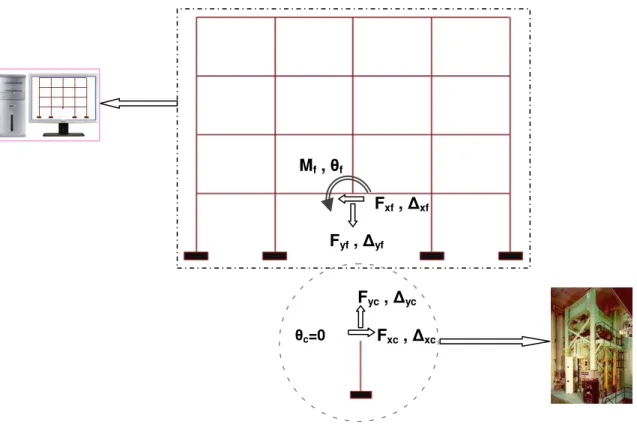
Figure 1 shows interaction components between the column specimens and the frame for a simple 2D system, which are Fxf, Δxf ,Fyf, Δyf, Mf, and θf, for the frame and Fxc,
Δxc ,Fyc, Δyc ,Mc, and θc, for the column correspondingly. In the case of the 3D frame,
these components are also required in the direction of and about the third axis, Z.
To satisfy equilibrium conditions, all the forces in the two directions of X and Y and the moment in Figure 1 must be identical, respectively.
Fxf = Fxc (1-1)
Fyf = Fyc (1-2)
Mf = Mc (1-2)
For compatibility conditions, all the displacements in the two directions of X and Y and the rotation in Figure 1 must be identical respectively.
Δxf = Δxc (2-1)
Δyf = Δyc (2-2)
The equilibrium and compatibility conditions need to be satisfied at each time step during the test. To do so, an iteration process will be carried out during the test as described later in this report.
FIGURE 1. Simplified HFT Method for a Middle Column.
Simplified HFT process for a column with insignificant rotation: middle columns
Figure 1 shows interaction components between the column specimens and the frame for a simple system. The components are Fxf, Δxf ,Fyf, Δyf, Mf, and θf for the frame
and Fxc, Δxc ,Fyc, Δyc,Mc, and θc for the column. In the case of the 3D frame, the
complements related to the third axis direction Z is also included.
For simplicity, it is assumed that θc=0 in Figure 1. For the frames with relatively
large stiffness compared to that of the column specimen, the connection may not need
to be restrained. However, for small frames, θf, should be zero as well. This would be a
reasonable assumption for a middle column with connections that are resisting with small rotations. Therefore, in such a case, no rotation or moment will be included, as interaction components, in the iteration process during the test. For a corner or end column where rotations are considerable larger, this assumption does not apply. For such columns a more general approach, explained later in this report, could be applied. In the case of applying the HFT for a 3D frame, all the three moment components of the three main axes at the end of the column specimen are assumed zero. The verification for this assumption is made for the 3D 6-storey building later in this report.
To satisfy both compatibility and equilibrium conditions for the frame in Figure 1, either load-controlled or displacement-controlled method could be employed for the column specimen and the frame. In other words, if the axial load for the column
Fxf , Δxf Fyf , Δyf Fxc , Δxc Fyc , Δyc Mf , θf θc=0
specimen, Fyc, is controlled during the test then the vertical deformation of the frame, Δyf,
needs to be controlled in the analysis/simulation. The inverse controlling method could be applicable as well, that is to control the axial deformation of the column specimen,
Δyc, in the test and to control the vertical force of the frame, Fyf, in the
analysis/simulation. However, for this test, the axial load of the column was controlled rather than the axial deformation. This method was chosen since the column could be very sensitive to the change in the axial deformation and there could be a possibility of high variation in the axial load at each iteration until the conversion is achieved. For lateral component, the same concept, either load-controlled or displacement-controlled method, can be applied. For this test, a displacement-controlled method was employed.
That is to control the lateral deformation of the column specimen, Δxc, and to control the
lateral force of the frame, Fxf in the analysis/simulation. The later method was selected,
because if the lateral load drops, at the post-peak stage of the column lateral load
capacity, the test could be continued to obtain the post peak response of the column.
HFT Steps – simplified method
Here are the steps for implementation of the HFT:
Step 1 Run analysis for the entire structure under required design load, with the column
specimen included in the analysis, at the initial stage or ambient temperature and
obtain Fxf0, Δxf0, Fyf0, and Δyf0 for the frame, the same components as that in
Figure 1.
Step 2 Run another analysis/simulation for the structure, but this time without the
column specimen and the frame is subjected to Fxf0, and Δyf0. Then the results for
the lateral deformation, Δxf, and vertical force, Fyf, should be identical or close to
the initial values, Δxf0, and Fyf0, obtained from step 1. If not, then increase or
reduce the Fxf0, and Δyf0, as required and repeat the above analysis until Δxf= Δxf0,
and Fyf= Fyf0 are achieved. This step may be necessary, since for simplicity, no
moment interaction is considered at the top of the column specimens. This will adjust the column axial load and lateral deformation to be the same as that of the whole frame. Such a difference, adjusted through this step, is usually very small and could even be ignored.
Note: Rotations are considered zero for the column specimen. In the case of rotations at the frame, they could be restrained to zero, which is the case for this test, or with no rotation restraint as the floor stiffness for rotation is significantly larger than that of the column specimen.
Step 3 For the column specimen in the furnace, apply the initial column’s axial load, Fyc0,
obtained from step 2, gradually, based on the rate required by the
CAN/ULC-S101 standard, until it reaches Fyf0. Then impose the initial lateral deformation,
Δxc0, gradually to reach Δxf0 on the column to. The test is now ready to start.
Step 4 Start the fire in the furnace for the column specimen
Step 5 Read Δyct, and Fxct, of the column specimen at time = t. Then run the
analysis/simulation for the frame, in Figure 1, while it is subjected to Δyft = Δyct,
and Fxft = Fxct. The results of the analysis will include Δxft, and Fyft at time = t.
Step 6 Adjust the axial load and lateral deformation for the column specimen in the
furnace with the numerical results obtained in step 5. That is Fyct = Fyft, and Δxct =
Δxft.
Step 7 Repeat steps 5 and 6 for each time increment, Δt, for the entire period of the test
including the cooling phase. Δt depends on the level of the acceptable error.
For the purpose of this test Δt was approximately 5 minutes, which provided a reasonable accuracy.
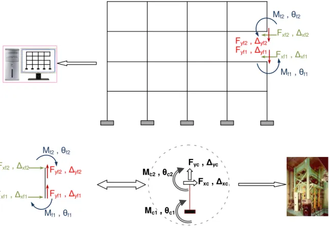
HFT general process,
The simplified HFT method is applicable only for columns with insignificant ends rotation, those are mostly middle columns. However, for a corner column, the rotations could be considerable large and such an assumption would not be applicable.
FIGURE 2. HFT Method.
Figure 2 illustrates a corner column on the third floor of a frame with force, moment, displacement and rotation components.
Equilibrium conditions require:
Fxc = -Fxf1 = Fxf2 (3-1) Fyc = -Fyf1 = Fyf2 (3-2) Mc1 = Mf1 , Mc2 = Mf2 (3-3) Fxc , Δxc Fyc , Δyc Mc2 , θc2 Mc1 , θc1 Fxf2, Δxf2 Fxf1 , Δxf1 Mf2, θf2 Mf1, θf1 Fyf2, Δyf2 Fyf1 , Δyf1 Fxf2, Δxf2 Mf2 , θf2 Mf1 , θf1 Fxf1, Δxf1 Fyf2 , Δyf2 Fyf1 , Δyf1
Compatibility conditions yield to:
Δxc = Δxf2 - Δxf1 (4-1)
Δyc = Δyf2 – Δyf1 (4-2)
θc1 = θf1 , θc2= θf2 (4-3)
HFT – general method application challenges
The NRC column furnace facility has been designed for the capability of applying
moment Mc, or rotation θc at both ends of the column specimen. However, such
capability needs to be commissioned. Until then, an equivalent approach could be employed to include the column’s end rotation. The equivalent method is described in the next section.
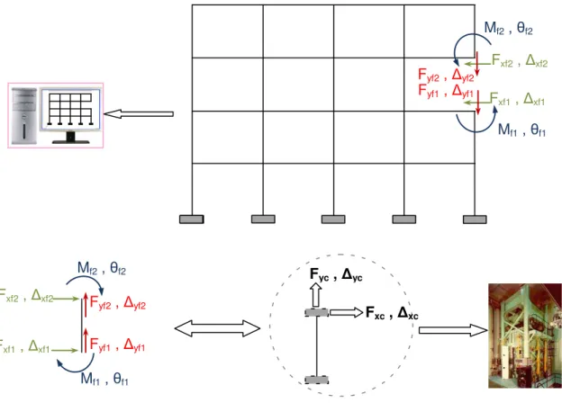
HFT – equivalent general method
The HFT equivalent approach is similar to the general method, except that for the column specimen in the furnace the column end rotations will be compensated by
adding an equivalent lateral displacement. Figure 3 illustrates the HFT equivalent method.
FIGURE 3. Equivalent General HFT Method.
In other words, while rotations at both ends of the column specimen are zero, the column is subjected to the axial load obtained from the frame reaction and a lateral displacement that is the sum of the lateral deformation of the frame and the equivalent displacement obtained from the applied rotation as described here.
Fxc , Δxc Fyc , Δyc Fxf2 , Δxf2 Fxf1, Δxf1 Mf2 , θf2 Mf1, θf1 Fyf2 , Δyf2 Fyf1, Δyf1 Fxf2 , Δxf2 Mf2, θf2 Mf1 , θf1 Fxf1, Δxf1 Fyf2 , Δyf2 Fyf1, Δyf1
Columns are all considered vertical elements with no applied load along their length except at the two ends.
Hence, relationships between forces and displacements of such a column specimen can be determined by Equation (5-1).
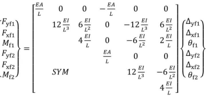
⎩ ⎪ ⎨ ⎪ ⎧��yf1 xf1 �f1 �yf2 �xf2 �f2⎭ ⎪ ⎬ ⎪ ⎫ = ⎣ ⎢ ⎢ ⎢ ⎢ ⎢ ⎢ ⎢ ⎢ ⎡��� 0 0 − �� � 0 0 12�� �3 6 �� �2 0 −12 �� �3 6 �� �2 4�� � 0 −6 �� �2 2 �� � �� � 0 0 ��� 12�� �3 −6���2 4�� � ⎦ ⎥ ⎥ ⎥ ⎥ ⎥ ⎥ ⎥ ⎥ ⎤ ⎩ ⎪ ⎨ ⎪ ⎧∆∆yf1 xf1 �f1 ∆yf2 ∆xf2 �f2⎭ ⎪ ⎬ ⎪ ⎫ (5-1)
From Equation (5-1), relations between lateral load and moment can be derived as:
� �xf1 �f1 �xf2 �f2 � =���3� 12 6� −12 6� 6� 4�2 −6� 2�2 −12 −6� 12 −6� 6� 2�2 −6� 4�2 � � ∆xf1 �f1 ∆xf2 �f2 � (5-2)
FIGURE 4. Equivalent Column Ends Conditions.
Column A in Figure 4 has general displacement and rotation conditions. Based on Equation (5-1) axial loads can be treated separately and are not included here. For Column A, based on the relation provided by Equation (5-2), lateral loads and moments are obtained. Mf1= (6∆xf1+4θf1L-6∆xf2 +2θf2L) EI /L 2 (6-1) Mf2= (6∆xf1+2θf1L-6∆xf2 +4θf2L) EI /L 2 (6-2) Mf2, θf2 Fxf2, ∆xf2 Fxf1, ∆xf1 Mf1, θf1 Column A M M Fxc, ∆xc Column B Fxc L
Fxf1= -Fxf2= 6EI[2(∆xf1-∆xf2) +θf1L+θf2L]/L 3
(6-3) Column B has the same conditions as the column specimen in Figure 3 with zero
end rotations and zero bottom-end’s lateral dispalacement. Lateral loads and moments for Column B are given below:
M= 6EI ∆xc /L 2
(7) Fxc = 12 EI ∆xc /L3
To have equivalent load conditions for Column A and B, lateral loads for both columns must be the same. This results to the following compatibility condition:
If Fxc = Fxf2 then ∆ xc =-[(θf1+θf2) L/2 +(∆xf1-∆xf2)] (8)
In other words, in order to compensate the employed rotation to the column
ends, additional lateral displacement of (θf1+θf2) L/2 must be added to the column’s initial
lateral displacement of (∆xf1-∆xf2).
Equivalent average moment for column specimen is:
M=-(Mf1+Mf2)/2 (9)
A useful moment factor used later in this report is R which is defined as:
From (6) R= Mf1/ Mf2 ={(3∆xf1-3∆xf2 +2θf1L +θf2L) / (3∆xf1-3∆xf2+θf1L+2θf2L)} (10)
Based on the above applied equilibrium conditions, lateral load and
displacements are the same for both Column A and Column B. As well, total rotations at the inflection points of Columns A and B and the sum of the end moments are the same. Although rotations and moments at the individual ends are different, this may have a very slight effect on the response simulation of the frame. Since the total rotation can be determined, rotation at one end of the column on the frame can be obtained by
deducting the rotation of the other end from the frame analysis, from the total rotation. The only consideration would be at the ultimate stage. In other words, as in the case of Column A moment at one end is larger than the average moment in Column B, faster failure may occur at that end of Column A than that of the Column B. However, it would not affect the overall failure of the column. This is because the failure would start from one end of Column A but after reaching the plastic moment at this end, the moment will be constant until the other end reaches its plastic moment capacity. Since both ends have the same plastic moment capacities then both will have similar moments at the failure stage.
Mu=-(Mf1u+Mf2u)/2= -Mf1u/2= -Mf2u/2 (11)
Therefore, moments for both Columns A and B are in equilibrium conditions at the failure stage, except the small difference during the plastic hinging transition. On the other hand, since shear load due to the moment rotation, in fire, would be a fraction of the total shear force of column, such difference is even smaller and can be ignored.
If the column fails in shear or shear-flexural, since both Columns A and B have the same shear stress along the columns, this would result again in a similar failure load. Total axial deformation of the column is the same for columns A and B due to similar total rotations at the inflection point, as they follow the same curvature, hence, axial
shear flexure interaction effects would also be included in the response (Mostafaei and Kabeyasawa, 2007).
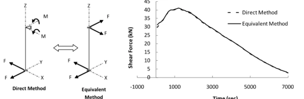
Above equilibrium conditions and method is verified for a 6-storey building prototype later in this report. The above approach can be applied based on the same concept for a bi-axial lateral loading. Figure 5 shows results of an analysis for a reinforced concrete column with a cross section of 305mm by 305mm and length of 3.8m with fixed bottom end. The top of the column was once subjected to rotation for both horizontal axes and the shear reactions of the column were obtained. Then based on the above equivalent technique, the top of the column was subjected to lateral loads with the same magnitude in the two directions, and the shear responses were
determined. As illustrated in Figure 5, a good agreement was achieved for both methods, when the initial system was subjected only to the rotations and when the equivalent system was subjected to the lateral loads. The figure shows the column’s shear force in each direction.
FIGURE 5. Shear Response, F, of a Reinforced Concrete Column, Calculated Using the Direct Method and the Equivalent Approach.
HFT Steps – equilibrium general method
Here are the steps for the implementation of the HFT equilibrium general method.
Step 1 Run analysis/simulation for the entire structure, including the column specimen,
at the initial stage or ambient temperature and obtains Mfi, θfi, Fxfi, Δxfi, Fyfi, and
Δyfi, where, i = 1,2, see Figure 3. Then determine the column specimen load and
deformation components, Fxc0, Δxc0, Fyc0, and Δyc0 at the ambient temperature.
Fxc0 = -Fxf1 = Fxf2 (12-1)
Fyc0 = -Fyf1 = Fyf2 (12-2)
Δyc0 = Δyf2 – Δyf1 (12-3)
∆ xc0 = -[(θf1+θf2) L/2 +(∆xf1-∆xf2)] (12-4)
Above equation is a sign sensitive. Follow the signs in Figure 4 for the positive and negative directions.
Step 2 For the column specimen in the furnace, apply the initial column’s axial load, Fyc0,
obtained from step 1. Then impose the column to the initial lateral deformation,
Δxc0. The test is now ready to start.
Step 3 Start the fire in the furnace for the column specimen.
Step 4 Read Δyct and Fxct, of the column specimen at time = t. Include P-Δ effects on
lateral load due to eccentricity of the axial load for the additional lateral
Direct Method Equivalent Method X Y Z M M X Y Z F F F F F F 0 5 10 15 20 25 30 35 40 45 -1000 1000 3000 5000 7000 S h e a r F o rc e ( kN ) Time (sec) Direct Method Equivalent Method
deformation due to the rotation Equation (13-2). Then, run the analysis/simulation for the frame in Figure 3 while it is subjected to:
Fyf1= Fcy (13-1)
Fxf2 = Fxct + [Fyct(θf1+θf2) L/2]/L (13-2)
Fxf1= Fxf2 (13-3)
Δyf2= Δyct + Δyf1 (13-4)
From (9) and (10) Mf1 = - 2M/(1+R) and Mf2 = Mf1/ R (13-5)
The results of the analysis/simulation will include Δxf1, Δyf1, θf1, Δxf2,θf2,Fyf2 at time = t.
Step 5 For the column specimen in the furnace, employ the obtained column’s axial
load, Fyc = Fyf2,and lateral deformation, Δxc using Equation (8).
Step 6 Repeat steps 4 to 5 for each time increment, Δt, for the entire period of the test
including the cooling phase. Δt is depending on the level of the acceptable error.
A SIX-STOREY REINFORCED CONCRETE BUILDING FOR HFT
A 6-storey reinforced concrete building was designed based on the Canadian Building Code, for design loads, and Concrete Design Standard for a hybrid fire test. The objective of the test was commissioning the HFT and verifying application of the HFT method in practice.
Building Configuration
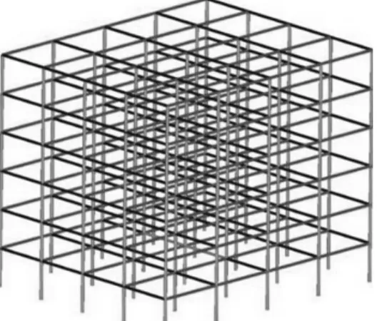
Figure 6 shows the overall configuration of the building structure.
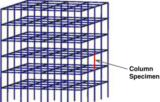
FIGURE 6. The 6-Story Prototype Reinforced Concrete Building Structure.
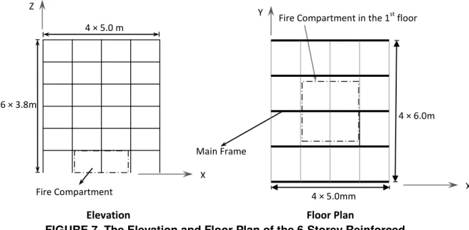
A fire compartment scenario being in the centre of the first floor is presumed for this test. Figure 7 shows both the floor plan of the building and the elevation of the main frame as well as the location of the fire compartment in the first floor. The main frames of the building are in the direction with the shorter spans (5.0m), as shown in Figure 7. The frames perpendicular to the main frames are considered secondary frames. The floor loads are considered to be carried only by the main frames.
Design Criteria
Applied Load
The building is assumed as a commercial building located in Ottawa, Canada. The dead load, live load and the snow load were determined according to the 2010 National Building Code of Canada (NBCC) for different floors. Then the factored loads were calculated based on the CAN/ULC-S101 standard for fire resistance tests. The resulting factored uniformed distributed load to be applied at the building roof level during the fire test, was determined as 7 (kPa). The factored uniformed distributed load to be applied on the other floor levels was obtained at 11 (kPa). With the span of 6.0 m, the main mid frames at the roof level were subjected to 42 kN/m and the main mid frames at other levels to 66kN/m. The end frames were subjected to half of the above loads accordingly, since they carry loads of only half span.
FIGURE 7. The Elevation and Floor Plan of the 6-Storey Reinforced Concrete Building.
Previously, a reinforced concrete column was tested using the traditional prescriptive method under a constant load of 2000kN. For the sake of comparison, the applied load was adjusted in order to achieve the same level of axial load in the centre column of the first floor. 3D structural analyses were carried out for the building, until the above axial load was achieved. The new applied load obtained for the main mid frames at the roof level was 43.7 kN/m and that for the main mid frames at the other levels was 68.5kN/m. The end frames were subjected to half of the above loads accordingly. The new loads were larger than the initial calculated loads based on CAN/ULC-S101 standard; therefore the applied loads were more than the minimum required load.
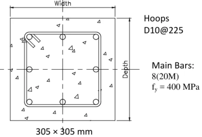
Column sections
As mentioned previously, a reinforced concrete column was tested using the traditional prescriptive method under a constant load. For the sake of comparison, the second column specimen, with identical properties, was chosen for this test. The column specimens were 3.8m long with a cross section, the details shown in Figure 8. Concrete compressive strength measured 96 MPa based on three cylinder compression tests,
Fire Compartment in the 1st floor
4 × 5.0mm
4 × 6.0m
Main Frame
Elevation Floor Plan
X X Z Y 6 × 3.8m 4 × 5.0 m Fire Compartment
carried out before the fire test. The concrete was made of siliceous aggregates with a mix of still fibre, 42kg per cubic meter.
Beam sections
The same concrete properties were considered for beams as that for columns. Figure 9 shows the cross section for the beams of the main frames with material
properties for concrete and steel. Figure 10 illustrates the cross section for beams in the secondary frames. In order to include stiffness of the floor slabs in the analysis, all beams were designed as T beams. For simplicity, end beams were modeled with the same cross sections as that of the mid beams.
FIGURE 8. Cross Section of Columns at all Levels.
FIGURE 9. Cross Section of Beams in the Main Frames.
FIGURE 10. Cross Section of Beams in the Secondary Frames.
Hoops D10@225 Main Bars: 8(20M) fy = 400 MPa 305 × 305 mm Hoops D10@200 Main Bars: 4(25M) fy = 400 MPa 150 mm 500 mm 300 mm 500 mm 50 mm Hoops D10@200 Main Bars: 4(15M) fy = 400 MPa 150 mm 250 mm 200 mm 600 mm 50 mm
Assumptions
Mechanical properties of the concrete for all sections were identical with 96MPa compressive strength concrete. All the reinforcement steel had 400MPa yielding stress. The numerical analyses were carried out using SAFIR software. Beams and columns were simulated using fibre models and therefore shear responses of the elements were ignored. All the connections were considered moment resisting connections.
The fire compartment was considered to be at the centre of the building, therefore, lateral deformations due to thermal expansion could be ignored. This assumption is verified later in this report. A future study will test an end/corner column with lateral load deformation interactions included. The column specimen was fixed at the top end for rotation. The interaction components between the column specimen and the frame were the column end’s axial load and axial deformation.
VERIFICATION OF THE SIMPLIFIED METHOD
Few assumptions were made in the simplified HFT method. The main assumption is that all the rotations at the top end of the column specimens are
considered zero. In order to verify this assumption, three 3D numerical analyses were carried out for the 6-storey reinforced concrete building prototype, shown in Figure 6, using the SAFIR structural analysis software. For the purpose of comparisons,
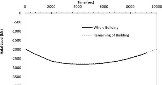
CAN/ULC-S101 fire was selected as the design fire, since the same fire was employed previously for fire resistance of structural assemblies using traditional testing approach. 1) Simulated analysis for the whole building, while all the floor elements and the column in the fire compartment were exposed to the CAN/ULC-S101 fire. The results included axial load of the column in the fire compartment and its top-end vertical deformation at different time steps.
2) Simulated analysis of the building, but without the column specimen while it was subjected to the column’s top-end vertical deformation, obtained in analysis (1),
determined the corresponding reaction which is Fyf. The frame was imposed to zero
rotations at the node, where the column was separated. Figure 11 illustrates comparison
of the axial load of the column when being part of the whole building and Fyf was
obtained from this analysis. Figure 12 shows both the obtained top-end vertical
deformation of the column from analysis (1) and the employed Δyf for this analysis. The
difference between the two curves is 0.075mm during the entire test which is due to the implemented load adjustment. The adjustment of the initial load was made as described previously in the HFT steps.
3) Simulated analysis of the single column specimen when it was subjected to the axial load of the column obtained from analysis 1 and determined vertical
deformation of the column specimen, Δyc. Zero rotations were imposed at the top of the
column. This simulates the same boundary conditions as that of the column in the NRC’s column furnace. Figure 13 shows axial load obtained from analysis (1) and the vertical
load applied in this analysis on the column specimen Fyc. Figure 14 illustrates the
comparison of the axial deformation at the top end of the column, when being part of the
whole building, analysis (1), and the vertical displacement of the column specimen, Δyc,
FIGURE 11. Axial Load of the Column when Being Part of the Whole Building and Fyf Obtained from the Analysis of the Building without the Column.
FIGURE 12. Top End Vertical Deformation of the Column when Being Part of the Whole Building and Δyf imposed to the Building without the Column.
FIGURE 13. Axial Load in the Column Specimen for Both when it is Separated and When it is Part of the Whole Building.
Lateral deformations at the top-end of the column, when it was part of the whole building, obtained from the analysis (1), were negligible. Therefore, no lateral
displacement was applied for analyses (2) and (3).
Analyses (2) and (3) are simulating the HFT method. Therefore, since the Fyf
obtained in analysis (2) is matching the column axial load obtained from analysis (1),
Figure 11, and Δyc obtained in analysis (3) is matching that of analysis (1) for the whole
building, In Figure 14, the verification is achieved and the assumptions of zero rotations are confirmed. -4000 -3500 -3000 -2500 -2000 -1500 -1000 -500 0 0 2000 4000 6000 8000 10000 A x ia l L o ad ( k N ) Time (sec) Whole Building Remaining of Building -2 -1 0 1 2 3 4 0 2000 4000 6000 8000 10000 A x ia l De fo rm a tio n ( m m ) Time (sec) Whole Building Remaining of Building -2900 -2700 -2500 -2300 -2100 -1900 -1700 -1500 0 2000 4000 6000 8000 10000 A x ia l L o a d ( k N ) Time (sec) Whole Building Column Specimen
FIGURE 14. Top End Vertical Deformation of the Column Specimen for Both when it is Separated and When it is Part of the Whole Building.
VERIFICATION OF THE EQUIVALENT METHOD
Further numerical analyses were carried out using the HFT equivalent method to validate the applicability of the proposed process. At this time, an end column on the third floor of the building was chosen as the column specimen. Figure 15 shows the building with the location of the column specimen.
FIGURE 15. The 6-Storey Prototype Building with an End Column Specimen on the 3rd Floor.
In this case, the fire compartment is located on the third floor as shown in Figure 16. All the beams and the column in the fire compartment were exposed to the CAN/ULC-S101 standard fire.
Three analyses were carried out:
1) Simulated analysis for the whole building, while the structural elements in the fire compartment were exposed to the CAN/ULC-S101 fire and obtained axial load, shear force, end-moments, top-end and bottom-end displacements and rotations of the column in the fire compartment, referred to as the column specimen. Considering the location of the fire compartment, only displacements in the directions of X and Z axes, Δxf1, Δxf2, Δzf1, Δzf2, and rotations about Y axis, θyf1, θyf2, and their corresponding forces,
Fxf1, Fxf2, Fzf1, Fzf2, and moments, Myf1, Myf2, at the top and bottom ends of the column
were obtained. In other words, only components related to the main frame are
considered and the problem can be treated in two-dimension. Fzf1, and Fzf2, are in fact
-2 -1 0 1 2 3 4 0 2000 4000 6000 8000 10000 A x ia l De fo rm a tio n ( m m ) Time (sec) Whole Building Column Specimen Column Specimen
axial loads of the column Fzf1 = Fzf2. Fxf1 and Fxf2 are shear forces of the column. Shear
forces at both ends could have different values due to the P-Δ effect. Average value of
Fxf1 and Fxf2 were considered as the average shear force in the column specimen.
Note: For this analysis, remaining components of the deformations, Δyf1, Δyf2, θxf1,
θxf2, θzf1, θzf2, and their corresponding loads and moments were found negligible. In the
case of a corner column specimen, Δyf1, Δyf2, θxf1, θxf2, need to be included in the
analysis. However, the same process described here could be employed. Effects of torsions in the column were considered negligible. This would be a reasonable
assumption for conventional columns, where, due to relatively long length, compared to its cross sections dimensions, torque could be ignored.
FIGURE 16. The Elevation and Floor Plan of the 6-Storey Reinforced Concrete Building
2) Simulated analysis of the single column specimen when it was subjected to axial load, Fzc = Fzf2, lateral deformation, ∆ xc = -[(θyf1+θyf2) L/2 +(∆xf1-∆xf2)] based on the
results in analysis (1) and obtained Fxf2 = Fxct + [Fyct (θyf1+θyf2) L/2]/L, Δzc and
end-moments Mf1 and Mf2. It is important to use the right signs, positive or negative, for the
variables in these equations to obtain the proper results. Figures 17, 18 and 19 show the results of axial deformation, shear force and moment obtained from this analysis
compared with that from the whole building analysis, analysis (1), which indicates a good agreement. Moments were calculated using Equation (13).
3) Simulated analysis of the building but without the column specimen, Figure 15, while it was subjected to Fxf2 and Fxf1= -Fxf2, Fzf2=Fzc, and Δzf2= Δzc, obtained from
analysis (2). No other force, moment, deformation or rotation is imposed on the frame.
One may subject the frame also to Myf1 and Myf2 both calculated by Equation (13) from
analysis (2), however, for a large frame, where stiffness of the column compared to that of the whole building is very small, this could be ignored. For the purpose of comparison, analyses were carried out here with and without including the moment interactions between the column specimen and rest of the building.
X X
Z
Y Fire Compartment in the 3st floor
4 × 5.0mm 4 × 6.0m Main Frame Elevation Floor Plan 6 × 3.8m 4 × 5.0 m Fire Compartment
FIGURE 17. Top End Vertical Deformation of the 3rd Floor’s Column Specimen for Both when it is Separated and When it is Part of the Whole Building.
FIGURE 18. Average Shear Force of the 3rd Floor’s Column Specimen for Both when it is Separated and When it is Part of the Whole Building.
FIGURE 19. End-Moments of the 3rd Floor’s Column Specimen Obtained from Analysis of the Whole Building and Calculated using Equation (13).
Figures 20-23 show vertical and lateral displacements and rotations at the top and bottom ends of the column and its axial load obtained from the analysis of the whole building, analysis (1), and from the analysis of the building without the column specimen,
-2 0 2 4 6 8 10 12 14 0 3600 7200 10800 14400 A x ia l D is p l. (m m ) Time (sec) Whole Building Column Specimen -15 -5 5 15 25 35 45 0 3600 7200 10800 14400 S h e a r F o rc e ( k N ) Time (sec) Column Specimen Whole Building -100 -80 -60 -40 -20 0 20 40 60 80 100 0 3600 7200 10800 14400 M o me n t ( kN .m) Time (sec) Whole Building Column Specimen Top End Bottom End
analysis (3), which all show good agreements. These figures illustrate the results with no moment interaction between the column specimen and the rest of the building. In order to assess how effective it is to include moment interactions, an analysis was carried out
for the rest of the building when Myf1 and Myf2, calculated by Equation (13), were applied
to the top and bottom ends on the frame. Figure 24 illustrates the results of this analysis. It indicates a better correlation compared to that in Figure 22. However, the difference is not very significant. Note that the equivalent HFT can be applied with or without moment interactions. The advantage of not having moment interaction included in the analysis is less variable involved and less errors. Moments are sign sensitive and therefore more effort would be needed to make sure the top and bottom column ends are subjected to the correct moments and directions.
FIGURE 20. Top and Bottom Ends Vertical Deformation of the Column when Being Part of the Whole Building and for the Building without the Column.
FIGURE 21. Top and Bottom Ends Lateral Displacement of the Column in X direction when Being Part of the Whole Building and for the Building without the
Column Specimen. IMPLEMENTATION OF THE HFT
A Hybrid Fire Testing method was implemented using the method described in this report for a middle column. The results of the test will be published in a separate report. -6 -4 -2 0 2 4 6 8 10 12 14 0 3600 7200 10800 14400 A x ia l D is p l. (m m ) Time (sec) Whole Building Remaining of Building Top End Bottom End 0 10 20 30 40 50 0 3600 7200 10800 14400 La te ra l D is p l. X ( mm) Time (sec) Remaining of Building Whole Building Top End Bottom End
FIGURE 22. Top and Bottom Ends Rotations of the Column about Y Axis when Being Part of the Whole Building and for the Building without the Column
Specimen – With no Moment Interaction.
FIGURE 23. Axial Load of the Column when Being Part of the Whole Building and for the Building without the Column Specimen.
FIGURE 24. Top and Bottom Ends Rotations of the Column about Y Axis when Being Part of the Whole Building and for the Building without the Column
Specimen – With Moment Interaction.
-0.009 -0.008 -0.007 -0.006 -0.005 -0.004 -0.003 -0.002 -0.001 0.000 0 3600 7200 10800 14400 Ro ta ti o n ( Ra d ) Time (sec) Remaining of Building Whole Building Top End Bottom End Top End Bottom End -1,400 -1,200 -1,000 -800 -600 -400 -200 0 0 3600 7200 10800 14400 A x ial L o ad ( k N ) Time (sec) Remaining of Building Whole Building -0.009 -0.008 -0.007 -0.006 -0.005 -0.004 -0.003 -0.002 -0.001 0.000 0 3600 7200 10800 14400 Ro ta ti o n ( Ra d ) Time (sec) Remaining of Building Whole Building Top End Bottom End Top End Bottom End
CONCLUSION
A Hybrid Fire Testing method was developed for performance evaluation of structures in fire. A 6-storey reinforced concrete building was designed for the purpose of commissioning the HFT. Two methods, simplified and equivalent approaches were developed for middle columns and end columns of buildings. Both methods were
validated using the results of a 3D analysis of the whole building, analysis of the column when separated from the building and that of the rest of the building, without the column. The numerical results indicate that the equivalent method could provide reliable results as that of the full simulation. The advantage of the equivalent method is that the column furnace does not require to have a facility to apply support rotations. In other words, if a column testing facility only has the capability of applying axial and lateral loading, a column at any location in the building can be simulated using the equivalent HFT method while it shows comparable accuracy as that of the full simulation.
REFERENCES
1. Dermitzakis, S.N., Mahin, S.A. “Development of substructuring techniques for
on-line computer controlled seismic performance testing”. Report UBC/EERC-85/04, Earthquake Engineering Research Center, University of California, Berkeley, 1985.
2. Kaveh, A., Bahreininejad, A., Mostafaei, H. "Hybrid graph-neural method for
domain decomposition," International Journal Computers & Structures, 70, pp. 667-674, 1999.
3. Mostafaei, H., Mannarino, J. “A Performance -based approach for fire-resistance
test of reinforced concrete columns”, NRC-IRC Research Report 287, Sep 2009, pp. 22.
4. Mostafaei, H. “NRC-IRC develops new approach for structural fire resistance”,
Construction Innovation, Vol. 15, Issue 1, March 2010 (
http://www.nrc-cnrc.gc.ca/eng/ibp/irc/ci/v15no1/8.html ).
5. Mostafaei, H. and Kabeyasawa, T. (2007). “Axial-shear-flexure interaction
approach for reinforced concrete columns.” ACI Struct. J., 104(2), 218–226.
6. CAN/ULC-S101, “Fire Endurance Tests of Building Construction and Materials”,
Underwriters’ Laboratories of Canada, Scarborough, ON.
7. SAFIR, A Thermal/Structural Program Modelling Structures under Fire, Franssen
J.-M., Engineering Journal, A.I.S.C., Vol 42, No. 3 (2005), 143-158, http://hdl.handle.net/2268/2928.