Etude de quelques problèmes fractionnaires non linéaires

(1)

République Algérienne Démocratique et Populaire

Ministère de l’Enseignement Supérieur

et de la Recherche Scientifique

Université 8 Mai 1945 Guelma

Faculté de Mathématiques et d’Informatique

et des Sciences de la Matière

Laboratoire de Mathématiques Appliquées et Modélisation

Département de Mathématiques

Thèse :

Présentée en vue de l’obtention du diplôme de

Doctorat 3

ème

cycle en Mathématiques

Option :

Mathématiques Appliquées

Par : Abdourazek Souahi

Intitulée

Etude de quelques problèmes

fractionnaires nonlinéaires

Sous la direction de : M.C.A. Amara HITTA.

Co-encadreur : Prof.

Rabah KHALDI.

Devant le jury:

Président :

n

Fateh Ellaggoune

not

Prof.

not

Univ-Guelma.

Examinateur :

Assia Guezane-Lakoud

Prof.

U.B.M. Annaba.

(2)

Algerian Democratic and Popular Republic

Ministry of Higher Education

and Scientific Research

University of 8 May 1945 Guelma

Faculty of Mathematics and Informatics

and Matter Sciences

Laboratory of Applied Mathematics and Modeling

Department of mathematics

Thesis:

Presented for obtaining the degree of

3

rd

cycle Doctorate in Mathematics

Option:

Applied Mathematics

Presented by: Abdourazek Souahi

Intitulated:

Study of some nonlinear

fractional differential problems

Supervisor: M.C.A. Amara HITTA.

Co-Supervisor: Prof.

Rabah KHALDI.

Jury members:

President:

n

Fateh Ellaggoune

not

Prof.

not

Univ-Guelma.

Examiner:

Assia Guezane-Lakoud

Prof.

U.B.M. Annaba.

(3)

I, Abdourazek Souahi declare that this thesis and the work presented in it are my own and has been generated by me as the result of my own original research:

Study of some nonlinear fractional differential problems.

I confirm that:

• This work was done wholly or mainly while in candidature for a Ph.D. degree at this University;

• Where any part of this thesis has previously been submitted for a degree or any other qualification at this University or any other insti-tution, this has been clearly stated;

• Where I have consulted the published work of others, this is always clearly attributed;

• Where I have quoted from the work of others, the source is always given. With the exception of such quotations, this thesis is entirely my own work;

• I have acknowledged all main sources of help;

• Where the thesis is based on work done by myself jointly with others, I have made clear exactly what was done by others and what I have contributed myself.

Signed: ...

(4)

ﺺﺨﻠﳌﺍ

ﺖﻬﲡاو .ﺔﻳﴪﻜﻟا ﺔﻴﻠﺿﺎﻔﺘﻟا تﻻدﺎﻌﳌا ﺔﺳارﺪﺑ ﲔﺜﺣﺎﺒﻟا مﲈﺘﻫﺎﺑ نﺎﺗﲑﺧﻷا نﺎﺘﻳﴩﻌﻟا تﺰﻴﲤ

ﺾﻌﺑ .لﻮﻠﳊا راﺮﻘﺘﺳا لﻮﺣ تاﺮﻳﺪﻘﺘﻟا ﺾﻌﺑ ﻚﻟﺬﻛو ﺎﳍ لﻮﻠﺣ دﻮﺟوو ﺔﻴﻧاﺪﺣو ﰲ ﻢﲥﺎﺳارد

.ﺔﻴﺑﺎﺒﻀﻟا ﺔﻳﴪﻜﻟا تﻻدﺎﻌﳌاو ﺔﻴﻄﳋا ﲑﻏ تﻻدﺎﻌﳌا لﻮﺣ ترﻮﺤﲤ لﺎﺠﳌا اﺬﻫ ﰲ تﺎﳘﺎﺴﳌا

ﺎﺻاﻮﺧ ﺎﳍ ٍتﺎَﻴْﻨُﺒﻛ ةﺪﻫﺎﺸﳌا ﺮﻫاﻮﻈﻟا ﺔﺟﺬﻤﻧ ﰲ تﻻدﺎﻌﳌا ﻪﺗﺎﻫ ةرﺪﻗ ﱃإ ﻚﻟذ ﰲ ﻞﻀﻔﻟا ﻊﺟﺮﻳ

.ﺔﻤﻳﺪﻘﻟا ﺎﲥﻻﺎﺣ ﻦﻋ تﺎﻣﻮﻠﻌﻤﺑ ﻆﻔﺘﲢ داﻮﻣ تاﲑﻐﺗ ﺔﺟﺬﻤﻧ ﺪﻨﻋ ﺎﻬﺘﻴﳘأ ﺮﻬﻈﺗ ﲈﻛ ،ﺔﻴﻌﺿﻮﻣ ﲑﻏ

تﻻدﺎﻌﳌا ﺾﻌﺑ ﺔﺳارد لﻼﺧ ﻦﻣ ﻚﻟذو ،لﺎﺠﳌا اﺬﻫ ﰲ ﺔﳘﺎﺴﳌا ﻮﻫ ﺔﺣوﺮﻃﻷا هﺬﻫ ﻦﻣ فﺪﳍا

طوﴩﻟا ﺾﻌﺑو ،ةﺪﻣﺎﺼﻟا ﻢﻴﻘﻟا تﺎﻨﻫﱪﻣ ﺾﻌﺑ ﻞﻤﻌﺘﺴﻨﺳ .خﺎﻨﺑ تاءﺎﻀﻓ ﰲ ﺔﻳﴪﻜﻟا ﺔﻴﻠﺿﺎﻔﺘﻟا

.ﻮﻣﻮﻗﺎﻧ طوﴩﻟ ﺔﲠﺎﺸﳌا

اﺬﻛو ﺔﻴﺋاﺪﺘﺑﻻا ﻢﻴﻘﻟا تاذ تﻻدﺎﻌﳌا ﺾﻌﺒﻟ ﺔﺒﺟﻮﳌا لﻮﻠﳊا دﻮﺟو ﱃإ ﺮﻣﻷا ﺔﻳاﺪﺑ ﰲ قﺮﻄﺘﻨﺳ

ﺾﻌﺑ لﻮﻠﺣ ﺔﻴﻧاﺪﺣﻮﺑ ﻢﺘﳖ ﻢﺛ .ﻮﻴﻏو ﲇﺴﻟﺎﺳﻮﻨﺳاﺮﻛ ﺔﻨﻫﱪﻣ لﲈﻌﺘﺳﺎﺑ ﺔﻳﺪﺣ ﻢﻴﻗ تاذ تﻻدﺎﻌﻣ

ﺔﻴﺑﺎﺒﺿ ﻞﺋﺎﺴﻣ ﺔﳉﺎﻌﻣ ﰲ ﻢﻫﺎﺴﻨﺳ ﲑﺧﻷا ﰲ .ﻮﻣﻮﻗﺎﻨﻟ ﺔﲠﺎﺸﻣ طوﴍ لﲈﻌﺘﺳﺎﺑ ىﺮﺧﻷا تﻻدﺎﻌﳌا

.ﺎﳍﻮﻠﺣ ﺔﻴﻧاﺪﺣوو دﻮﺟو ﺔﻨﻫﱪﺑ ﺔﻴﻔﻴﻛ ﺔﻳﴪﻛ ﺐﺗر تاذ

.ﺔﻠﻤﻌﺘﺴﳌا تﺎﻴﻨﻘﺘﻟا ﺔﻴﻟﺎﻌﻓو ﺔﺤﺻ ﺮﻳﱪﺘﻟ ﺎﻴﻤﻗر ﻻﺎﺜﻣو ﺔﻴﺤﻴﺿﻮﺘﻟا ﺔﻠﺜﻣﻷا ﺾﻌﺑ ﻖﻓﺮﻨﺳ

:ﺔﻴﺣﺎﺘﻔﻣ ﺕﺎﻤﻠﻛ

تﺎﺒﻳﺮﻘﺗ ،ﺔﻴﻟﺎﺘﺘﳌا ﺐﻳرﺎﻘﺘﻟا ،ﺔﻴﻧاﺪﺣﻮﻟا ﺔﻨﻫﱪﻣ ،ﺔﻴﻄﺧ ﲑﻏ ﺔﻟﺄﺴﻣ ،ﺔﻳﴪﻛ ﺔﻴﻠﺿﺎﻔﺗ تﻻدﺎﻌﻣ

ﻂﻘﻨﻟا ﺔﻨﻫﱪﻣ ،ﺔﺒﺟﻮﻣ لﻮﻠﺣ ،ﺔﻴﻧاﺪﺣو ،دﻮﺟو ،ﺔﻳﺪﺣ طوﴍ ،ﺔﻴﺋاﺪﺘﺑﻻا طوﴩﻟا ،درﺎﻜﻴﺑ

طوﴍ ،ﻦﻳاﺮﻛو ﻲﻜﺴﻟﺎﺳﻮﻨﺳاﺮﻛ طوﴍ ،ﺔﻴﺑﺎﺒﺿ ﺔﻴﻠﺿﺎﻔﺗ تﻻدﺎﻌﻣ ،ﺔﻳﴪﻛ ﺔﻘﺘﺸﻣ ،ةﺪﻣﺎﺼﻟا

،ﻞﻴﻓﻮﻴﻟو نﲈﻳر ﺐﺴﺣ ﰊﺎﺒﻀﻟا ﻞﺿﺎﻔﺘﻟا ،ﻮﻴﻏو ﲇﺴﻟﺎﺳﻮﻨﺳاﺮﻛ ﺔﻧﱪﻣ ،سﺮﻏور طوﴍ ،يﻮُﻛ

.ﺔﻴﺑﺎﺒﺿ ﺔﻘﺘﺸﻣ

(5)

Abstract

In the last decades, the qualitative and the quantitative aspect of fractional differential equations got a lot of researchers’ attention. Some of the con-tributions in this fields are in the investigation of solutions to nonlinear fractional differential equations and fuzzy fractional differential equations. The interest in this field is mainly due to the large applicability of the the-ory in modeling problems presenting nonlocal characteristics, such as vis-coelasticity and memory preservation.

The object of this thesis is to contribute in the field of fractional calculus where we study some class of fractional differential equations in Banach spaces. Our results are based on fixed point theorems and Nagumo like conditions.

First, we establish the positivity and existence to a class of fractional initial value problems and boundary value problems using the fixed point theo-rem of Guo-Krasnoselskii. Later on, we establish the uniqueness along-side the existence of the solution of some initial value problems under Krasnoselskii-Krein like conditions. Finally, we are concerned by the study of a class of fuzzy fractional differential equations with uncertainty and we prove some new results on existence and uniqueness of high order prob-lems.

One numerical example and several other examples are provided to out-line the applicability and the usefulness of our results in the field.

Keywords:

Fractional differential equation ; Nonlinear problem ; Uniqueness theo-rem ; Successive approximations ; Picard’s iterates ; Initial value problem ; Boundary value problem ; Existence ; Uniqueness ; Positivity of solution ; Fixed point theorem ; fractional derivative ; Fuzzy fractional differential equations ; Krasnoselskii-Krein conditions ; Kooi conditions ; Rogers con-ditions ; Guo-Krasnoselskii Theorem ; Riemann-Liouville fuzzy differen-tiability ; Fuzzy derivative ; Fuzzy fractional differential equation.

(6)

Résumé

Ces deux dernières décennies ont connu un développement rapide dans la théorie du calcul fractionnaire. De nombreux chercheurs ont apporté des contributions importantes à cette théorie qui permet de mieux expliquer et modéliser les phénomènes non-locaux qui préservent une certaine mé-moire. L’intérêt est surtout porté à l’étude qualitative et quantitative des solutions de problèmes fractionnaires et de quelques équations différen-tielles fractionnaires floues.

Cette thèse est consacrée à l’étude de quelques problèmes engendrés par des équations différentielles d’ordre non entier. On s’intéresse à l’existence, à l’unicité et à la positivité de la solution. En se basant sur les théorèmes du point fixe et les méthodes itératives. On établit aussi quelques résultats pour les équations différentielles floues.

D’abord, on présente des résultats de positivité et d’existence de solutions de quelques classes d’équations différentielles fractionnaires de Riemann-Liouville, notamment à conditions initiales ou aux limites en utilisant le théorème du point fixe de Guo-Krasnoselskii. Ensuite, on établit l’existence et l’unicité avec d’autres techniques reposant sur des conditions semblables à celle de Nagumo. Enfin, quelques nouveaux résultats d’existence et d’uni-cité de solutions floues sont démontrés.

Pour bien illustrer leur applicabilité et leur intérêt particulier, on présen-tera quelques exemples et un cas numérique pour conclure.

Mots clés:

Equation différentielle fractionnaire ; Problème non linéaire ; Théorème d’unicité ; Approximations successives ; Itérations de Picard ; Conditions initiales ; Conditions aux limites ; Existence ; Unicité ; Positivité ; Théorème du point fixe ; Dérivée fractionnaire ; Equations différentielles fraction-naires floues ; Dérivée floue ; Conditions de Krasnoselskii-Krein ; Condi-tions de Kooi ; CondiCondi-tions de Rogers ; Théorème de Guo-Krasnoselskii ; Différentiabilité floue au sens de Riemann-Liouville.

(7)

To Allah. The Glorified and Exalted, The only One worshipped, The greatest Cherisher and Sustainer. For his satisfaction, I have read and written. He is the Best Disposer of affairs. And, Him alone is sufficient for us. May Him accept us as his righteous slaves and submitters, and pious worshippers. All the praises to Allah. My Almighty, Allah.

(8)

Acknowledgments

First, I would like to express my sincere gratitude to my mother and my father thought for sure, I would never be able to repay them. May them be proud of me.

Next, I would like to thank deeply my supervisor Dr. Amara Hitta for accepting to advise this thesis and supporting me with choosing the final objective of this research. In Annaba, Prof. Rabah Khaldi was the one that introduced me to the fractional calculus during my Master degree prepa-ration and co-advised this research, I gladly acknowledge and thank them.

Prof. Assia Guezane-Lakoud is a teacher and adviser who collaborated with me on this conducted research from its beginning. She showed great patience and understanding with me, I thank her very much.

Prof. Fateh Ellaggoune, Dr. Abderrazek Chaoui, and Dr. Khaled

Bouk-errioua are kindly thanked for accepting to be member of the jury, they honored me.

I would like to thank Dr. Badreddine Meftah, Prof. Lamine Nisse, Dr.

Rezgui Chemlal, and Dr. Khaled Boukerrioua for their contagious enthu-siasm that pushed me and guided me these couple years. Specially Dr. B.

Meftahfor his stimulating discussion in our meetings.

Also, I can’t thank enough my teachers, some of my friends, and the mem-bers of the Laboratory of Applied Mathematics and Modeling,

Labora-tory of Advanced Materials, and Preparatory School Science and

Tech-nology (EPST)where most of my exchanges and debates took place. They were very constructive and useful for me, thank you very much. Also, I’m very grateful to all the mathematicians I met during my studies and in particular at Sfax’ university: Prof. Mohammed Ali Hammami, Dr.

Ab-dellatif Ben-Makhlouf, Dr. Bassem Bennaser, Mr. Anis Dhifaoui, and many others.

(9)

I am deeply thankful to my mother and to my father in particular and to all the other member of my family they didn’t spare any unwavering support in any possible manner and I owe them an immeasurable debt of gratitude. I almost get short of words, so I thank anyone who helped me in any kind or manner as little as it can be, be it in the redaction of this thesis or along my research time. May I raise to the better of all their expectations.

(10)

List of Figures

1.1 Plot of the gamma function. . . 2

1.2 Crisp VS fuzzy membership logic. . . 17

1.3 Example of a crisp membership function. . . 19

1.4 Example of a fuzzy membership function. . . 19

(13)

List of Tables

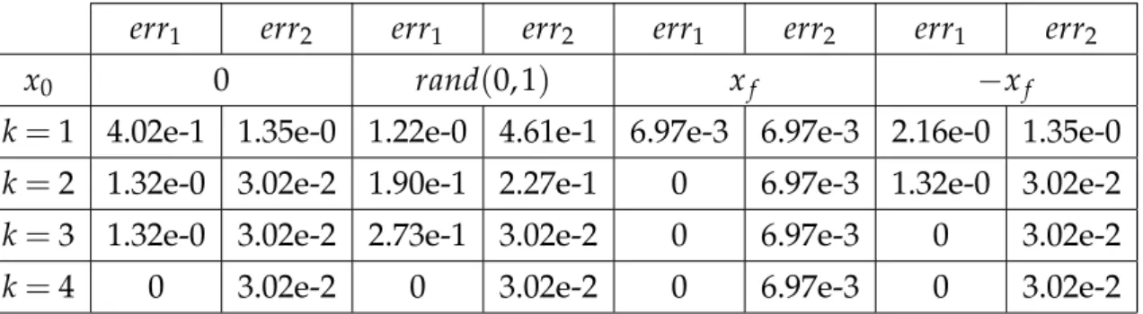
3.1 err1and err2for some values of x0. . . 65

(14)

List of Symbols

Symbol Description

FDE Fractional Differential Equation

FFDE Fuzzy Fractional Differential Equation

IVP Initial value problem

FIVP Fuzzy initial value problem

BVP Boundary value problem

Γ(·) Gamma function

β(·) Beta function

Cr_n, rCn Binomial coefficients

Eα(·) One-parameter Mittag-Leffler function

E_α,β(·) Two-parameter Mittag-Leffler function

GL_Dα _{Grunwald-Letnikov fractional derivative}

Iα Fractional Riemann-Liouville integral

Dα Fractional Riemann-Liouville derivative

R_Dα _{Fractional Riesz derivative} C_Dα _{Fractional Caputo derivative}

Re(·) Real part of the complex variable

[·] Integer part of the real variable

{·} Fractional part of the real variable

AC Space of absolutely continuous functions

L1 Space of Lebesgue integrable functions

, Denoted by

(15)

L−1 _{Inverse Laplace transform}

L Fuzzy Laplace transform

d(·,·) A metric or Hausdorff distance (in fuzzy sets)

D(·,·) Another distance defined in the last chapter

E Space of fuzzy numbers

µ(·) Fuzzy membership function

⊙,⊕ Multiplication and addition in fuzzy sets

⊖ H-difference

CF Space of continuous fuzzy valued functions

LF Space of all Lebesgue integrable fuzzy valued functions

(16)

Author’s papers

[1] A. Souahi, A. Ben Makhlouf, and M. A. Hammami. Stability analysis of fractional-order nonlinear systems. Submitted.

[2] A. Souahi, A. Guezane-Lakoud, and A. Hitta. On the existence and uniqueness for high order fuzzy fractional differential equations with uncertainty. Advances in Fuzzy Systems, pages 9, 2016.

[3] A. Souahi, A. Guezane-Lakoud, and A. Hitta. Positive solutions for higher-order nonlinear fractional differential equations. Vietnam

Jour-nal of Mathematics, pages 1–10, 2016.

[4] A. Souahi, A. Guezane-Lakoud, and A. Hitta. Some uniqueness results for fractional differential equation of arbitrary order with nagumo like conditions. Thai Journal of Mathematics. In press.

[5] A. Souahi, A. Guezane-Lakoud, and R. Khaldi. On a fractional higher order initial value problem. Submitted.

[6] A. Souahi, A. Guezane-Lakoud, and R. Khaldi. On some existence and uniqueness results for a class of equations of order 0<α≤1on arbi-trary time-scales. International Journal of Differential Equations, pages 8, 2016.

(17)

Introduction

A huge number of physical phenomena is modeled using differential equa-tions. A great portion of the models has been or is being studied using the fixed point theory.

In the past years, researchers from around the world tried to narrow the gap of error between the physical model and the experiments conducted in adjacency. This resulted in the introduction and application of new the-ories or extension of old thethe-ories, such as time-scales theory, fuzzy sets theory, fractional calculus, etc.

The fractional calculus and fuzzy set theory caught our attention. In a mat-ter of fact, the former one is a generalisation of integration and differen-tiability to noninteger order numbers and was coined by Leibniz in his famous letter to L’Hôpital. With this theory, models have fewer variables and are better describing nonlocal properties and memory characteristics in models. The Latter theory was introduced by Zadeh and Klaua as an ex-tension of the classic notion of set. In contrast with the classical set theory where the elements either belong or don’t belong to the set, an element on fuzzy sets have a gradual membership with intermediate grades: rather belong than not, to more likely to be out of the set. In this suitable concept to cope with reality, the incomplete or imprecise information are better un-derstand and taken into account.

These theories advanced considerably the modeling and efficience of a wide range of applications, for instance signal processing, molecular

(18)

bi-ology, psychology analysis, game theory, etc.

Motivated by the works on these two theories and as a continuation of the works conducted intensively in these fields, our objectives are to demon-strate the existence and uniqueness of solutions for fractional differential equations with initial value problems and boundary value problem using the definition of Riemann-Liouville in crisp sets and fuzzy sets.

We treat in the chapters of this thesis the following problems under several assumptions. The several notation that arises are defined properly in the main chapters. { Dqx(t) = f(t, x(t), Dq−1x(t)) x(0) =0, D(q−i)x(0) =0, i=1, . . . ,[q],        Dqu(t) +g(t)f(u(t), u′(t), u′′(t), . . . , u(m)(t), Dαu(t)) =0, u(0) =0, u(i)(0) =0, i=1, . . . , n−2, Dβu(1) =0, 2≤β≤n−2, 1≤m≤α≤β−1, { Dqx(t) = f(t, x(t), Dq−1x(t)) x(0) =y0, D(q−i)x(0) = ˜0, i=1, . . . ,[q].

This thesis is organized as follows:

In the preliminaries’ Chapter of this thesis, we recall necessary definitions, notions, and two models. Chapter 2 is based on the papers submitted [96] and accepted [95]. We treat two FDE; one is with initial data and the sec-ond one is with boundary csec-onditions. After succinctly speaking about the previous researchs in the field, we give new results on the existence of pos-itive solutions. Further, in the following Chapter 3, we prove the existence of uniqueness for a class of FDE using different techniques than those of Chapter 2 and provide a numerical example, see the accepted paper [93]. At last, Chapter 4 is based on the accepted paper [94]. We use the fuzzy Laplace transform and Nagumo-like conditions to obtain several unique-ness results for fuzzy fractional differential equations of high order.

(19)

Chapter 1 Preliminaries

In this chapter, we give an introduction to the several concepts that are of a particular interest in what follows. First, we define the fractional differ-entiation and give some practical properties and lemmas. Next, we give some general definitions and some fixed point theorems. Finally, we intro-duce fuzzy sets and exhibit some extensions, definitions, and other useful theorems.

1.1 Fractional Calculus on crisp sets

1.1.1 Fractional differentiation and integration

Before introducing a definition of fractional derivative we define some special functions which generalise the factorial and exponential functions, more details on the book [2].

Definition 1.1.1(Gamma function)

The gamma functionΓ(·)is defined by the integral

Γ(z) =

∫ _∞

0 e

−t_tz−1_dt,

(20)

One of the basic properties of the gamma function is that it satisfies Γ(z+1) =zΓ(z),

and for every integer n≥0, we have

Γ(n+1) =n!.

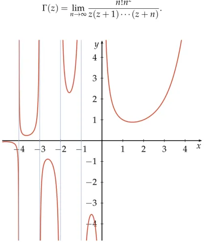
The gamma function can be represented also for every z∈ C such that Re(z) >0by the limit Γ(z) = lim n→∞ n!nz z(z+1)· · · (z+n). 1 2 3 4 −1 −2 −3 −4 1 2 3 4 −1 −2 −3 −4 x y

Figure 1.1: Plot of the gamma function.

Properties 1.1.2

(21)

(i) Γ′(x) >0, for every x>xmin >1,

(ii) x_min ≃1.461 andΓ(x_min)≃0.885,

(iii) Γ(1) =Γ(2) =1,

(iv) Γ(x)Γ(x−1) = π

sin(πx) for every0<x<1.

The binomial coefficients for r, n integers such that 0≤r≤n are defined

by

Cr_n=rCn= n! (n−r)!r!.

Without loss of generality, we denote by rCα the following extended bino-mial coefficients forα∈R+

rCα= Γ(α+1)

Γ(n−r+1)Γ(r+1).

Definition 1.1.3(Beta function)

For every z, w∈C such that Re(z) >0,Re(w) >0, the beta function is defined

by

B(z, w) =

∫ ₁

0 t

z−1₍₁₋_t₎w−1_dt.

An interesting formula relating the gamma and beta functions is

B(z, w) = Γ(z)Γ(w)

Γ(z+w).

Mittag-Leffler introduced a function that plays the role of the exponential function in the fractional calculus. Several generalisations were introduced by many researchers later. For the convenience of the reader, we define here briefly the one parameter and two parameters Mittag-Leffler func-tions. In [35, 71, 88, 89], several discussions and properties of this function could be found.

Definition 1.1.4(One-parameter Mittag-Leffler function)

(22)

by Eα(z) = ∞

∑

k=0 zk Γ(αk+1), whereα>0.

This function coincides with the exponential function whenα=1.

Definition 1.1.5(Two-parameter Mittag-Leffler function)

For everyα, β>0 and z∈R, the two parameter Mittag-Leffler function is defined

by Eα,β(z) = ∞

∑

k=0 zk Γ(αk+β).

A great number of papers and books on the theory and applications of fractional calculus appeared. They used several approaches to defining integration and differentiation of arbitrary order, see [38, 63, 74, 78, 82, 87]. The following are some of the most used ones:

Definition 1.1.6

The Grunwald-Letnikov fractional derivative of orderα>0 of f is given by

GL_Dα af(t) = lim h→0+ 1 hα [(t−a)/h]

∑

k=0 (−1)k(αCkf(t−kh).

Definition 1.1.7(Riemann-Liouville fractional integral)

The fractional integral of the function h:(0,∞)→R of order α∈R+ is defined by Iαh(t) = 1 Γ(α) ∫ _t 0 (t−s)α−1h(s)ds, provided the right side is pointwise defined on(0,∞).

Definition 1.1.8(Riemann-Liouville fractional derivative)

For a function h∈C((0,∞),R), the Riemann-Liouville fractional derivative of h

is defined by Dαh(t) = 1 Γ(n−α) ( d dt )_n_∫ _t 0 (t−s) n−α−1_h₍_s₎_ds,

(23)

where n∈N∗and n= [α] +1, provided that the right side is pointwise defined

on(0,∞).

Definition 1.1.9(Riesz fractional derivative)

The Riesz fractional derivative of fractional orderα of the function f is given by

R_Dα_f₍_t_{) =} −1 2 cos(πα/2)Γ(n−α) × dn dtn (_∫ _t −∞(t−s) n−α−1_f₍_s₎_ds_{+ (}₋₁₎n∫ +∞ t (t−s) n−α−1_f₍_s₎_ds ) . Definition 1.1.10

Letα>0 and n= [α] +1, for a function f ∈Cn([a, b],R)the Caputo fractional derivative of f of orderα is defined by

C_Dα_f₍_t_{) =} 1

Γ(n−α)

∫ _t

0 (t−s)

n−α−1_fn₍_s₎_s.

Lemma 1.1.11(Relation between RL and C derivatives)

Letα≥0 and n= [α] +1. Assume that h :[a, b]→R is such that Dαh and Dnh exist. Then C_Dα_h₍_t_{) =}_Dα_h₍_t₎₋

_∑

n k=0 Dkf(a) Γ(k−α+1)(x−a) k−α_.

In the realm of fractional differential equations, the most used definitions are Caputo and Riemann-Liouville derivatives. The Caputo definition is more welcome due to initial data in integer derivatives, Nevertheless, the Riemann Liouville derivatives are possible to measure and observe as can be found in [57]. Furthermore, fractional order initial conditions of Riemann-Liouville type differential equations can be given by integer order condi-tions, as usual, see [68, 104]. For the above mentioned reasons, we will focus on it throughout this manuscript. And we refer the reader to the good monographs and book [1, 63, 67, 82, 87], for discussions and more details on the fractional calculus.

Lemma 1.1.12([63])

Let p, q≥0 and f ∈L1([0, 1]), then

(24)

and

DqI₀q₊h(t) =h(t).

Lemma 1.1.13([63])

Let p>q>0, and h∈L1([a, b]), then for all t∈ [a, b]we have DqI₀p₊h(t) = I₀p₊−qh(t).

Theorem 1.1.14(Leibniz’ formula for Riemann-Liouville operators)

Let n>0 and assume that f and g are analytic on(a−h, a+h)with some h>0.

Then, Dα[f g](t) = [α]

∑

k=0 Cn_k(Dkf)(t)(Dα−kg)(t) + ∞

∑

k=[α]+1 C_kn(Dkf)(t)(Ik−αg)(t), for a<t<a+h₂.

Ifα, β∈C such that Reβ>0, then

1. (I_aα₊(t−a)β−1)(x) = _Γ₍Γ_β(₊β)_α₎(x−a)β+α−1 (Reα>0) 2. (Dα_a+(t−a)β−1)(x) = Γ (β) Γ(β−α)(x−a)β−α−1 (Reα≥0) 3. (I_bα₋(b−t)β−1)(x) = _Γ₍Γ_β(₊β)_α₎(b−x)β+α−1 (Reα>0) 4. (Dα_b₋(b−t)β−1)(x) = _Γ₍Γ_β(₋β)_α₎(b−x)β−α−1 (Reα≥0).

Remark1.1.15. Unlike the usual differentiation, the fractional derivative in Riemann-Liouville sense of a constant is not zero. However

(Dα_a+tα−m)(x) =

Γ(α−m+1)

Γ(n−m+1)(x

n−m₎(n) ₌

0,

for every m∈ {1, 2, . . . ,[Reα] +1}. This last equation will be used in proving the equivalence between FDE and the associated integral equation.

(25)

1.1.2 Fractional functional spaces

Before speaking of a solution to differential equations, we need the func-tional space were the solution belongs to obtain some regularity proper-ties. The problems treated in the following chapters use some of the Ba-nach spaces defined in this subsection or based on the definitions below. The list here is not exhaustive and we refer to some books devoted to this branch [36, 48].

We denote by AC(0, 1) the space of absolutely continuous functions defined on

[0, 1]. In fact, x∈ AC(0, 1)if and only if there existϕ∈ L1((0, 1),R)and c∈R such that

x(t) =c+

∫ _t

0 ϕ(s)ds for t∈ (0, 1),

where L1([0, 1],R)is the Banach space of Lebesgue integrable functions from[0, 1]

intoR with the norm∥h∥_L1 =

∫₁

0 |h(t)|dt. Also, we define ACn−1(0, 1)by

ACn−1(0, 1) ={x∈Cn−2, x(n−1)∈ AC(0, 1)}.

Theorem 1.1.17([83, Theorem 7.21])

If x:[a, b]→R is differentiable at every point of[a, b]and x′∈L1on[a, b], then x(t)−x(a) =

∫ _t

a x

′₍_τ₎_dτ.

Theorem 1.1.18([47, Theorem 3.21])

If x:[a, b]→R, the followings are equivalent:

(i) x is absolutely continuous on[a, b].

(ii) x(t)−x(a) =∫_aty(τ)dτ for some y∈L1([a, b],R).

(iii) x is differentiable almost everywhere on[a, b], x′∈L1([a, b],R), and x(t)−x(a) =∫_atx′(τ)dλ(τ).

(26)

1.1.3 Between the FDE and the integral equation

The basic idea of this subsection is to get general results of the following classical standard result from differential and integral calculus.

Theorem 1.1.19(Fundamental Theorem of classical calculus)

Let f :[a, b]→R be a continuous function and F :[a, b]→R be defined by

F(t),

∫ _t

a f(s)ds.

Then, F is differentiable and F′= f . Lemma 1.1.20([63])

Assume that u∈C(0, 1)∩L1(0, 1)with a fractional derivative of orderα>0 that

belongs to C(0, 1)∩L1(0, 1), then

I₀α+D0α+u(t) =u(t) +C1tα−1+C2tα−2+. . .+Cntα−n

for some C_i∈R, i=1, 2, . . . , n.

Lemma 1.1.21([63])

Forα>0, the general solution of the fractional differential equation D₀α₊u(t) =0

is given by u(t) =C₁tα−1+C2tα−2+. . .+Cntα−n, where C_i∈R, i=1, 2, . . . , n, and n= [α] +1. Lemma 1.1.22 Let v∈ L1((0, 1),R), then u(t) = 1 Γ(q) ∫ _t 0 (t−s)q−1v(s)ds is the unique continuous solution on[0, 1]of the equation

D₀q₊u(t) =v(t), (1.1)

satisfying the initial conditions

(27)

Proof. In fact, we may apply Lemma 1.1.20 to reduce equation (1.1) to an equivalent integral equation

u(t) = I₀q₊v(t) +C₁tq−1+C2tq−2+. . .+Cntq−n,

for some C_i, i=1, . . . n.

By the initial conditions u(0) =0, D(q−i)u(0) =0, i=1, . . . ,[q], we obtain

C1=C2=··· =Cn=0.

Substituting theses values in the last formula, we obtain the expression of the unique solution of (1.1) subject to the conditions (1.2)

u(t) = 1

Γ(q)

∫ _t

0

(t−s)q−1v(t)ds.

A function x is called a solution of the nonlinear equation

Dqu= f(t, u) (1.3)

where f is a continuous function an[0, 1], if x∈C([0, 1],R), Dqx exists and

is continuous on[0, 1], f(t, x)is well defined, and x satisfies (1.3).

It’s often the case to use some special transforms to obtain the associated integral equation, and one of the main methods is the Laplace transforms as mentioned by A. Jafarian et al. in [59].

We say that a function f : [0,∞) → E is of an exponential type, if there exist t0, M>0, andγ∈R such that

∥f(t)∥ ≤ Meγt, for all t≥t0.

In other words, the function f must not grow faster then a certain exponential function when t→∞.

(28)

Lemma 1.1.24

Let f : [0,∞)→E be a locally integrable function of an exponential type. Then there existsγ>0 such that

∫ _∞

0 e

−λt_f₍_t₎_dt

is convergent forRe(λ) >γ.

Denote the subset D by

D={f ∈L1((0,∞), E): f is of exponential type}.

Definition 1.1.25(Laplace transform)

The Laplace transformLof f ∈D is defined by

L{f(t)}{λ} =

∫ _∞

0 e

−λt_f₍_t₎_dt.

Definition 1.1.26(Inverse Laplace transform)

Let ˜f be an integral function. We define the inverse Laplace transform of ˜f by

L−1_{_˜f₍_λ₎_}{_t_{} =} 1

2πi

∫ _c+i∞

c−i∞ e

λt _˜f₍_λ₎_dλ.

1.2 Existence and uniqueness theorems

In general cases, when we want to study a fractional differential equation, we have to obtain solution in a suitable functional spaces. Later, we modify the problem suitably and apply one of the fixed point theorems in combi-nation with other useful estimates and known inequalities in order to es-tablish the wanted existence, uniqueness or stability results. In this Section, we recall some known fixed point theorems. We think that the books and notes [6, 28, 50, 56, 61, 67, 90] give sufficiently large number of theorems, other versions of these theorems, their proofs alongside applications of the theory.

(29)

1.2.1 Fixed point theorems

A mapping T of a metric space E into itself is said to satisfy a Lipschitz condition with a Lipschitz constant K if

d(Tx, Ty)≤Kd(x, y),

for every x, y∈E. If this condition is satisfied with 0≤K<1 then T is called a

contraction mapping.

Theorem 1.2.2(Banach’s contraction mapping principle)

Let(E, d)be a complete metric space and T be a contraction mapping from E into itself. Then T has a unique fixed point x0and for each x∈E, limn→∞Tn(x) =x0. Moreover, d(Tn(x), x₀)≤₁K₋n_kd(x, T(x)).

Theorem 1.2.3(Nonlinear alternative of Leray-Schauder [103])

Let E be a Banach space and C be a nonempty convex subset of E. Let U be a nonempty open subset of C with 0∈U and T : U→C continuous and compact operator. Then either

(1) T has fixed points or

(2) There exist u∈∂U and λ∈ (0, 1)such that u=λT(u). Theorem 1.2.4(Brouwer fixed point theorem)

Let B be a non empty compact convex subset of a finite dimensional normed space and let T be a continuous mapping of B into itself. Then T has a fixed point in B. Theorem 1.2.5(Schauder)

Let B be a non empty closed convex subset of a normed space. Let T be a continuous mapping of B into a compact subset of B, then T has a fixed point in B.

Theorem 1.2.6(Altman)

(30)

∥x∥ ≤r}and let T be a continuous mapping of Q into a compact subset of E such that

∥Tx−x∥2≥ ∥Tx∥2− ∥x∥2,

for every x verifying∥x∥ =r. Then T has a fixed point in Q. Theorem 1.2.7(Schaefer)

Let E be a normed space, T a continuous mapping of E into E which is compact on each bounded subset B of E. Then either

(i) the equation x=λTx has a solution for λ=1, or

(ii) the set of all such solution x, for0<λ<1, is unbounded.

Theorem 1.2.8(Krasnoselskii)

Let M be a closet convex non-empty subset of a Banach space(E, d). Suppose that A and B map M into E and suppose the following conditions are satisfied

(i) Ax+By∈M, for all x, y∈ M, (ii) A is compact and continuous, (iii) B is a contraction mapping.

Then there exists y in M such that Ay+By=y. Lemma 1.2.9(Arzelà-Ascoli Theorem)

LetΩ be a bounded subset of Rn. A subset A∈C(Ω)is relatively compact if and only if it is bounded and equicontinuous.

Lemma 1.2.10(Arzelà-Ascoli Theorem)

Let X be a compact metric space and Y any metric space. A subsetϕ of the space C(X, Y)of continuous mappings of X into Y is totally bounded in the metric of uniform convergence if and only ifΦ is equicontinuous on X and Φ(x) ={ϕ(x):

ϕ∈Φ}is a totally bounded subset of Y for each x∈X.

(31)

A closed subset P of a Banach space X is called a cone if: (i) ∀x, y∈P : x+y∈P,

(ii) ∀x∈P,∀α>0 :αx∈P, (iii) P∩ (−P) ={0}.

A cone P defines a partial order by x≤y⇔y−x∈P. Theorem 1.2.12(Guo-Krasnoselskii)

Let E be a Banach space and P⊂E be a cone. AssumeΩ1andΩ2are open bounded subsets contained in E with0∈Ω1andΩ1⊂Ω2. Assume, further, that

T : P∩(Ω2\Ω1

)

→P be a completely continuous operator. If either

(I) ∥Tu∥ ≤ ∥u∥, u∈ P∩∂Ω₁and∥Tu∥ ≥ ∥u∥, u∈P∩∂Ω2or (II) ∥Tu∥ ≤ ∥u∥, u∈ P∩∂Ω₂and∥Tu∥ ≥ ∥u∥, u∈P∩∂Ω₁. Then T has at least one fixed point in P∩(Ω₂\Ω₁).

1.2.2 Nagumo like theorems

Before stating some theorems, we would like to define some subsets. • S={(t, y)∈ [t₀−a, t₀+a]× [y₀−b, y₀+b]}.

• S0={(t, y)∈ [t0, t0+a]× [y0−b, y0+b]}.

• D0={(t, y): 0≤t≤a,|y| <∞}.

(32)

such that a, b>0and t0, y0≥0. Theorem 1.2.13(Lipschitz, 1876)

Let f be continuous and satisfies a Lipschitz condition with respect to x: that is,

|f(t, x)− f(t, x| ≤K|x−x|

in some neighbourhood V of (a, b). Then the differential equation with initial condition

dy

dt = f(t, y), y(a) =b (1.4) has a unique solution in some neighbourhood of a.

In the following some uniqueness theorems which assumes different con-ditions on the function f(·,·)then the Lipschitz condition.

Theorem 1.2.14(Peano’s Uniqueness Theorem)

Let f(t, y)be continuous in S0and nonincreasing in y for each fixed t∈ [t0, t0+a]. Then, IVP(1.4) has at most one solution in[t0, t0+a].

We say that a function f(·,·)satisfies Nagumo’s condition in a set D if

|f(t, y)− f(t, y)| ≤k|t−t₀|−1|y−y|, for all(t, y),(t, y)∈D, such that t̸=t₀and k≤1.

Theorem 1.2.15(Nagumo’s uniqueness theorem)

Let f(t, y)be continuous function, which satisfies Nagumo’s condition in S. Then, IVP(1.4) has at most one solution in|t−t0| ≤a.

The constant in the Nagumo condition k could be greater than 1 provided we add an additional condition, for proofs and other interesting results, see the excellent book of Agarwal et al. [4].

Theorem 1.2.16(Krasnoselskii-Krein’ Uniqueness theorem)

(33)

(i) |f(t, x)− f(t, x)| ≤k|t−t0|−1|x−x|, t̸=t0,

(ii) |f(t, x)− f(t, x)| ≤ c|x−x|α, where c and k are positive constants, the real numberα is such that 0<α<1, and k(1−α) <1.

Then IVP(1.4) has at most one solution in|t−t₀| ≤a. Theorem 1.2.17(Kooi’s Uniqueness theorem)

Let f(t, x)be a continuous function on S, which satisfies for all(t, x),(t, x)∈S: (i) |f(t, x)− f(t, x)| ≤k|t−t0|−1|x−x|, t̸=t0,

(ii) |t−t₀|β|f(t, x)−f(t, x)| ≤c|x−x|α, where c and k are positive constants, the real numberα is such that 0<α<1, β<α and k(1−α) <1−β.

Then IVP(1.4) has at most one solution in|t−t₀| ≤a. Theorem 1.2.18(Roger’s uniqueness theorem)

Let f(t, y)be continuous in D0, which satisfies the condition f(t, y) =o(e−1/tt−2)

uniformly, for0≤y≤δ, δ>0 arbitrary. Further, let

|f(t, y)−f(t, y)| ≤ 1

t2|y−y|, t̸=0

for all(t, y),(t, y)∈D0. Then IVP(1.4) has at most one solution in[0, a].

Consider the initial value problem

x′=h(t, x), x(t0) =x0 (1.5)

where h : U⊂Rn →R is continuous.

Theorem 1.2.19(Kamke’s uniqueness Theorem)

Assume that for all(t, x),(t, x)∈U, t̸=t₀, if

(34)

for some continuous function g:(0, a]× [0, 2b]→ [0,∞)such that for every c∈

(0, a), the trivial solution x≡0 is the only solution of

x′(t) =g(t, x(t)) for all t∈ (0, c), and lim

t→0+

x(t)

t =0. Then IVP(1.5) has at most one solution in[t0, t0+a].

Theorem 1.2.20(Montel-Tonelli uniqueness Theorem)

Assume that for all(t, x),(t, x)∈U, t̸=t₀, we have

|h(t, x)−h(t, x)| ≤ p(t−t₀)ψ(∥x−x∥),

where p:(0, a]→ (0,+∞)is integrable, andψ :[0, 2b]→ [0,+∞)is continuous

and _∫

0+

dr

ψ(r) = +∞.

Then IVP(1.5) has at most one solution in[t0, t0+a].

Last, we provide two inequalities that will be used in the sequel. The first is a particular case of Jensen’s inequality and the second in a generalisation of the Jensen’s inequality.

Lemma 1.2.21

For every a, b∈ (0, 1)and everyα≥1, we have the following estimate

(a+b)α≤2

α

2 (a

α₊_bα₎_.

Lemma 1.2.22(Jensen’s inequality [101])

Let p be a nonnegative continuous function on[a, b]such that∫_abp(x)dx>0.

If g and h are real-valued continuous functions on[a, b]and m1≤g(x)≤M1, m2≤h(x)≤M2, for all x∈ [a, b], and F is convex on

∆= [m1, M1]× [m2, M2], then F (∫_b a_∫g(t)p(t)dt b a p(t)dt , ∫_b a_∫h(t)p(t)dt b a p(t)dt ) ≤ ∫_b a F(g_∫(t), h(t))p(t)dt b a p(t)dt . (1.6)

(35)

1.3 Fuzzy sets

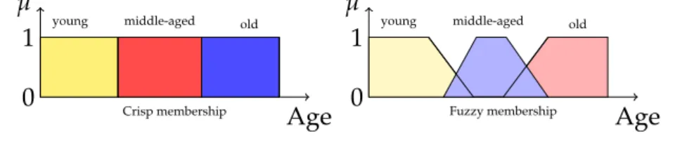
In contrast to odd and even numbers which can be classified as belonging to exactly one class, in many engineering tasks, we are faced with classes such as tall, speed, age, etc. All of these convey a useful semantic meaning that is obvious to a certain community. However, a borderline between the belonging or not of a given object to such classes is not evident. Two-valued logic, used in describing these classes of situations, might be not well-suited, see Figure 1.2.

Crisp membership _Age µ

0

1 young middle-aged old

Fuzzy membership

Age

µ

0

1 young middle-aged old

Figure 1.2: Crisp VS fuzzy membership logic.

1.3.1 Basic definitions and properties

First, let us recall some basic definitions about fuzzy numbers, fuzzy sets, and fuzzy logic. Further foundation and applications of this theory could be found in [64, 102, 113].

LetE={u :R→ [0, 1]; usatisfies (A1)-(A4)}the space of fuzzy numbers: (A1) u is normal: that is, there exists y₀∈R such that u(y₀) =1,

(A2) u is fuzzy convex i.e. u(λy+ (1−λ)z)≥min{u(y), u(z)}whenever

y, z∈R and λ∈ [0, 1],

(A3) u is upper semicontinuous i.e. for any y₀∈R and ϵ>0there exists

δ(y0,ϵ) >0such that u(y) <u(y0) +ϵ whenever|y−y0| <δ, y∈R,

(36)

The set[u]α={x∈R; u(y)≥α}is called anα-level set of u.

It follows from (A1)-(A4) that theα-level sets[u]αare convex compact sub-sets ofR for all α∈ (0, 1]. The fuzzy zero is defined by

˜0=    0 if y̸=0, 1 if y=0. Definition 1.3.1([113])

A fuzzy number u in the parametric form is a pair(u(r), u(r))of functions u, u, for0≤r≤1, which satisfy the following conditions:

(i) u is a bounded nondecreasing left continuous function in(0, 1] and right continuous at0,

(ii) u is a bounded nonincreasing left continuous function in(0, 1] and right continuous at0,

(iii) u(r)≤u(r), for all0≤r≤1.

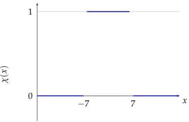
The characteristic function of a set D is denotedχ : D→ {0, 1}such that χ(x) =

{

1 if x∈D

0 if x /∈D.

Whereas a trapezoid fuzzy membership functionµ : D→ [0, 1]verifies

µ(x) =                0 if x≤a, x−a b−a if a≤x≤b, d−x d−c if c≤x≤d, 0 if d≤x,

such as[a, d]⊂D, below an other membership function is plot on Figure 1.4 and a crisp membership function on Figure 1.3.

Moreover, we also can present the r-cut levels of fuzzy numbers as[u]r= [u(r), u(r)]

(37)

−7 7 0 1 x χ ( x )

Figure 1.3: Example of a crisp membership function.

−7 7 0 1 x µ ( x )

Figure 1.4: Example of a fuzzy membership function.

According to Zadeh’s extension principle, we have the following proper-ties of fuzzy addition and multiplication by scalar onE

(u⊕v)(x) =sup y∈R min{u(y), v(x−y)}, x∈R, and (k⊙u(x)) =    u(x_k) if k≥0, ˜0 if k=0.

(38)

Seeking simplicity, we note⊕,⊙by the usual+,·. The Hausdorff distance between the fuzzy numbers is denoted by d :E×E→ [0,+∞[, such that

d(u, v) =sup_r_∈[_0,1_]max{|u(r)−v(r)|,|u(r)−v(r)|}. And (d,E) is a com-plete metric space.

Let x, y ∈ E. If there exists z ∈ E such that x = y+z, then z is called the Hukuhara difference of x and y, and it is denoted by x⊖y and called H-difference. Remark 1.3.3. Note that the sign ⊖ stands for H-difference and x⊖y ̸= x+ (−1)y.

We denote by CF[0, a] the space of all fuzzy-valued functions which are continuous on[0, a]and LF[0, a]the space of all Lebesgue integrable fuzzy-valued functions on[0, a], where a>0. We also denote by AC(n−1)F[0, a]

the space of fuzzy-valued functions f which have continuous H-derivati-ves up to order n−1on[0, a]such that f(n−1) in ACF[0, a].

1.3.2 Fuzzy differentiation and integration

Definition 1.3.4([26])

A function f : (a, b) →E is called H-differentiable on x₀ ∈ (a, b) if for h>0

sufficiently small there exist H-differences f(x0+h)⊖f(x0), f(x0)⊖f(x0−h) and an element f′(x0)∈R such that

0=lim h↘0d ( f(x₀+h)⊖ f(x₀) h , f ′₍_x 0) ) =lim h↘0d ( f(x₀)⊖ f(x₀+h) h , f ′₍_x 0) ) ,

where h at denominator means 1_h⊙.

This usual concept of differentiability has some shortcoming:

Remark1.3.5. If c is a fuzzy number and g :[a, b]→R an usual real valued

function differentiable on x₀∈ (a, b)with g′(x₀)≤0, then f(x) =c⊙g(x)

is not differentiable on x₀. In [26], Bede et al. defined a generalised concept of differentiability.

(39)

Let f :(a, b)→E and x₀∈ (a, b). We say that f is strongly generalised differen-tiable on x₀if there exists an element f′(x₀)∈E, such that for all h>0 sufficiently

small, we have (i) f′(x₀) =lim h→0 Φ(x₀+h)⊖Φ(x₀) h =lim h→0 Φ(x₀)⊖Φ(x₀−h) h , or (ii) f′(x0) =lim h→0 Φ(x0)⊖Φ(x0+h) −h =lim h→0 Φ(x0−h)⊖Φ(x0) −h . Definition 1.3.7([12])

Let f ∈CF[0, 1]∩LF[0, 1]. The fuzzy fractional integral of the fuzzy-valued func-tion f is defined by Iβf(x; r) = [ Iβf(x; r), Iβf(x; r) ] , 0≤r≤1, where Iβf(x; r) = 1 Γ(β) ∫ _x 0 (x−s) β−1_f₍_{s; r}₎_ds, Iβf(x; r) = 1 Γ(β) ∫ _x 0 (x−s)β−1f(s; r)ds.

Definitions for higher-order derivatives were introduced based on the se-lection of derivative type in each step of differentiation.

In [26], the authors considered four cases for derivative up to second order. Following [12] and for the sake of convenience, we only consider two cases. The other cases are trivial because they can be reduced to crisp elements. For more details, see [12].

(40)

Definition 1.3.8([12, Definition 6] )

Let f ∈C(n)F[0, 1]∩LF[0, 1], x0∈ (0, 1), andΦ(x) = (1/Γ(n−β))

∫_x

0(f(t)dt/(x− t)β−n+1), where n= [β] +1. We say that f is fuzzy Riemann-Liouville fractional

differentiable of order β at x₀, if there exists an element

(

D₀βf

)

(x₀) ∈E, such

that for all h>0 sufficiently small, we have

(i) ( D₀βf ) (x₀) =lim h→0 Φ(n−1)₍_x 0+h)⊖Φ(n−1)(x0) h =lim h→0 Φ(n−1)₍_x 0)⊖Φ(n−1)(x0−h) h , or (ii) ( D₀βf)(x₀) =lim h→0 Φ(n−1)₍_x 0)⊖Φ(n−1)(x0+h) −h =lim h→0 Φ(n−1)₍_x 0−h)⊖Φ(n−1)(x0) −h .

Denote by C(n−1)F([0, a])the space of fuzzy-value functions f on the inter-val[0, a]which have continuous H-derivative up to order n−2such that

f(n−1)∈CF[0, a]. C(n−1)F([0, a])is a complete metric space endowed by the metric D such that for every g, h∈C(n−1)F([0, a]):

D(g, h) = n−1

∑

i=0 sup t∈[0,a] d ( g(i)(t), h(i)(t) ) .

In the rest of this thesis, we say that a fuzzy-valued function f is RL[(i)−

β]-differentiable if it is differentiable as in Definition 1.3.8 case (i) and is

RL_[(_ii₎₋_β_]_{-differentiable if it is differentiable as in Definition 1.3.8 case}

(ii).

Definition 1.3.9([12, Theorem 7])

Let f ∈C(n)F[0, 1]∩LF[0, 1], x0∈ (0, 1), andΦ(x) = (1/Γ(n−β))

∫_x

0(f(t)dt/(x− t)β−n+1), where n= [β] +1 such that 0≤r≤1, then

(41)

(i) if f isRL[(i)−β]-differentiable fuzzy valued function, then ( D₀βf ) (x0; r) = [( D₀βf ) (x0; r), ( D₀βf ) (x0; r) ] , or

(ii) if f isRL[(i)−β]-differentiable fuzzy valued function, then

( D₀βf ) (x0; r) = [( D₀βf ) (x0; r), ( D₀βf ) (x0; r) ] , where ( D₀βf ) (x₀; r) = [ 1 Γ(n−β) ( d dx )_n_∫ _x 0 (x−t)n−β−1f(t; r)dt ] x=x0 ( D₀βf ) (x₀; r) = [ 1 Γ(n−β) ( d dx )_n_∫ _x 0 (x−t)n−β−1f(t; r)dt ] x=x0 .

1.3.3 High order differential equations and limitations

In [14], Allahviranloo and Ahmadi introduced the fuzzy Laplace trans-form, which they used under the strongly generalised differentiability. Re-cently, E. ElJaoui et al. [43] developed it further. The newly defined fuzzy Laplace transform [14] for high order fuzzy derivatives is one of the most useful methods as mentioned by A. Jafarian et al. in [59]: ”…, one of the important and interesting transforms in the problems of fuzzy equations is Laplace transforms. The fuzzy Laplace transform method solves fuzzy fractional differential equations and fuzzy boundary and initial value prob-lems [21, 22, 86] ….” See also [9, 85].

Let f be a continuous fuzzy-valued function. Suppose that f(x)⊙e−px is im-proper fuzzy Riemann integrable on[0,∞), then∫₀∞ f(x)⊙e−pxdx is called the fuzzy Laplace transform of f and is denoted by

L[f(x)] =

∫ _∞

0 f

(42)

Remark1.3.11. Using the definition of fuzzy Riemann integration, if follows that L[f(x)] = ( L[f(x, r) ] ,L [ f(x, r) ]) . Theorem 1.3.12

Let f′be an integrable fuzzy valued function and f its primitive on[0,∞). Then L[f′(x)] =p⊙L[f(x)]− f(0)

when f is (i)-differentiable or

L[f′(x)] = (−f(0))⊖ (−p⊙L[f(x)]).

when f is (ii)-differentiable.

Let us give the following theorem whose prove is essentially based on [12, Theorem 16]

Theorem 1.3.13

Suppose that f ∈C(n)F[0,∞)∩LF[0,∞), one has the following: (i) if f isRL[(i)−β]-differentiable fuzzy valued function, then

L [( D₀βf ) (x) ] =pβL[f(t)]⊖ ( n−1

∑

k=0 pkDβ−k−1f ) (0) or

(ii) if f isRL[(i)−β]-differentiable fuzzy valued function, then L [( D₀βf ) (x) ] =− ( n−1

∑

k=0 pkDβ−k−1f ) (0)⊖ ( −pβL[f(t)] ) .

For more details and properties of the fuzzy Laplace transform, we kindly refer the reader to [14, 43, 80] and for an application to fuzzy differential equations see, e.g., [17], Chapter 4, and the references cited therein.

(43)

Chapter 2 Existence of positive solutions in

a cone

The value of a mathematical discipline is to be de-termined by its applicability to the empirical sci-ences

C. Runge, Doctoral dissertation, Berlin, 23 April 1880.

Initial and boundary value problems of fractional orders have been stud-ied extensively in the last decades and by different methods, for instance, fixed point theorems, upper and lower solution method, coincidence de-gree theory of Mawhin.

In this Chapter, we establish sufficient conditions for the existence of pos-itive solutions for a class of higher order Riemann-Liouville fractional ini-tial and boundary value problems. By means of Guo-Krasnoselskii fixed point theorem, we investigate the existence of at least one positive solution in suitable cones. The first part is dedicated to the study of IVP where the second one is devoted to BVP.

(44)

2.1 Previews works

It goes without saying that ordinary and fractional IVP and BVP are greatly treated in several thousands of papers, we only cite a few: the works of Zhang et al. [105–111], Bai [24], Goodrich [49], Sotiris et al. [77], Guezane-Lakoud et al. [51–55], Chidouh et al. [31–33], others [69, 70, 98], and many more details in [3, 8] and the references cited therein. We give an overview of the problems treated:

In [7], Agarwal et al. treated the following boundary value problem

Dαu+ f(t, u(t), Dµu(t)) =0, 0≤t≤1, 1<α<2,

u(0) =u(1) =0,

withµ≤1−α and f satisfies Carathéodory conditions.

In [70, 98], the authors used Schauder fixed-point theorem for a coupled system where the nonlinear terms involve a fractional derivative of order 0<σ<1.

In [66], Lakshmikantham et al. obtained the existence uniqueness of solu-tion to the following IVP, using Krasnoselskii-Krein type condisolu-tions

D₀qu(t) = f(t, u(t)).

More details are in Chapter 3, when we treat a more general problem. In [24], Bai considered the existence of positive solutions of the fractional boundary value problem:

Dα₀u(t) + f(t, u(t)) =0, 0<t<1, 1<α≤2,

u(0) =0,βu(η) =u(1),

where D₀αdenotes the Riemann-Liouville fractional derivative. In [49], Goodrich studied a similar problem

−D₀νu(t) = f(t, u(t)), 0<t<1,

(45)

The author established the existence of a positive solution using cone the-oretic techniques.

In [77], Sotiris et al. extended his problem to a nonlinear fractional order differential equation with advanced arguments

Dα₀u(t) +a(t)f(u(θ(t))) =0, 0<t<1, n−1<α≤n, u(i)(0) =0, [ Dβu(t) ] t=1=0, 0≤i≤n−2, 1≤β≤n−2, n>3.

In [52], Guezane-Lakoud et al. studied the following problem

c_Dα

0u(t) = f(t, u(t), Dσ(t)), 0<t<1, 2<α<3, u(0) =u′(0) =u′′(0) =0, u′(1) =cDσu(1),

wherecD₀αrepresents the Caputo fractional derivative of orderα. And re-cently in [51], the author established the existence and uniqueness for the following problem

Dqu(t) = f(t, u(t), u′(t)), 0≤t≤1,

u(0) =u′(0) =u′′(0) =0,

where 2<q<3, using Guo-Krasnoselskii theorem.

Note that in the previously cited works and in many others, the authors trea-ted initial value problems assuming that the nonlinear term f depends on the classical derivatives of u, i.e. Diu for i ∈ N, or on the fractional

derivatives Dσu,σ∈]0, 1[, also they used some assumptions on the growth of a certain fractional derivative of the solution. In contrast to most of the anterior works, we prove the existence of at least one positive solu-tion without imposing a growth assumpsolu-tion on the fracsolu-tional derivative

Dq−1u.

A few question arises about quantitative aspect of positive solution in the following cases:

• The nonlinear term depends not only on integer derivatives of the solution but also on its fractional order derivative

(46)

• The fractional derivative that the nonlinear term depends on is of high order

Motivated by the active investigations on the IVP and BVP. In the follow-ing, we prove some existence results for two problems and answer some of the above questions. For that, first, we define some quantities and recall some lemma.

2.2 Some definitions

We set C0_u= [ Iq(1−t)−βg(t)f(u(t), u′(t), u′′(t), . . . , u(m)(t), Dαu(t)) ] t=1, Ci_u= Γ(q) Γ(q−i)C0, C α u = Γ(q) Γ(q−α)C0, Ru(t) = f(u(t), u′(t), u′′(t), . . . , u(m)(t), Dαu(t)), γ=min      ( 1 2 )_q₋_β₋₁ 2β−1 , ( 1 2 )q−1     . (2.1) Definition 2.2.1([99]) Let f :R2→R, define F∗:R+→R+, F∗(r) = max 0≤u+v≤r{f1(u, v)}, F0= lim |u|+|v|→0+ f₁(u, v) u+v , F ∗ 0 =lim_r_→₀ F∗(r) r , F∞ = lim |u|+|v|→+∞ f1(u, v) u+v , F ∗ 0 =_rlim_→_∞ F∗(r) r ,

The case where F0=∞ and F∞ =0 is called the sublinear case. Lemma 2.2.2([99, Lemma 2.8])