R. Ahuja, T. L. Magnanti, J. B. Orlin and M. R. Reddy
OF
NETWORK OPTIMIZATION
Ravindra K. Ahuja
Department of Industrial and Management Engineering
Indian Institute of Technology
Kanpur - 208 016, INDIA
Thomas L. Magnanti
Sloan School of Management
Massachusetts Institute of Technology
Cambridge, MA 02139, USA
James B. Orlin
Sloan School of Management
Massachusetts Institute of Technology
Cambridge, MA 02139, USA
M. R. Reddy
Department of Industrial and Management Engineering
Indian Institute of Technology
Kanpur - 208 016, INDIA
Highways, telephone lines, electric power systems, computer chips, water delivery systems, and rail lines: these physical networks, and many others, are familiar to all of us. In each of these problem settings, we often wish to send some good(s) (vehicles, messages, electricity, or water) from one point to another, typically as efficiently as possible-that is, along a shortest route or via some minimum cost flow pattern. Although these problems trace their roots to the work of Gustav Kirchhoff and other great scientists of the last century, the topic of network optimization as we know it today has its origins in the 1940's with the development of linear programming and, more broadly, optimization as an independent field of scientific inquiry, and with the parallel development of digital computers capable of performing massive computations. Since then, the field of network optimization has grown at an almost dizzying pace with literally thousands of scientific papers and multitudes of applications modeling a remarkably wide range of practical situations.
Network optimization has always been a core problem domain in operations research, as well as in computer science, applied mathematics, and many fields of engineering and management. The varied applications in these fields not only occur "naturally" on some transparent physical network, but also in situations that apparently are quite unrelated to networks. Moreover, because network optimization problems arise in so many diverse problem contexts, applications are scattered throughout the literature in several fields. Consequently, it is sometimes difficult for the research and practitioner community to fully appreciate the richness and variety of network applications.
This chapter is intended to introduce many applications and, in doing so, to highlight the pervasiveness of network optimization in practice. Our coverage is not intended to be encyclopedic, but rather attempts to demonstrate a range of applications, chosen because they are (i) "core" models (e.g., a basic production planning model), (ii) depict a range of applications including such fields as medicine and the molecular biology that might not be familiar to many readers, and (iii) cover many basic model types of network optimization: (1) shortest paths; (2) maximum flows; (3) minimum cost flows; (4) the assignment problems; (5) matchings; (6) minimum spanning trees; (7) convex cost flows; (8) generalized flows; (9) multicommodity flows; (10) the traveling salesman problem; and (11) network design. We present five applications for each of the core shortest paths, maximum flows, and minimum cost flow problems, four applications of the matching, minimum spanning tree, and traveling salesman problems, and three applications for each of the remaining problems.
The chapter describes the following 42 applications, drawn from the fields of operations research, computer science, the physical sciences, medicine, engineering, and applied mathematics:
1. System of difference constraints 2. Telephone operator scheduling 3. Production planning problems
4. Approximating piecewise linear functions 5. DNA sequence alignment
6. Matrix rounding problem 7 Baseball elimination problem
8. Distributed computing on a two-processor computer 9. Scheduling on uniform parallel machines
10. Tanker scheduling
11. Leveling mountainous terrain
12. Reconstructing the left ventricle from X-ray projections 13. Optimal loading of a hopping airplane
14. Directed Chinese postman problem 15. Racial balancing of schools 16. Locating objects in space 17. Matching moving objects 18. Rewiring of typewriters 19. Pairing stereo speakers 20. Determining chemical bonds 21. Dual completion of oil wells
22. Parallel saving heuristics
23. Measuring homogeneity of bimetallic objects 24. Reducing data storage
25. Cluster analysis
26. System reliability bounds 27. Urban traffic flows 28. Matrix balancing
29. Stick percolation problem
30. Determining an optimal energy policy 31. Machine loading
32. Managing warehousing goods and funds flow 33. Routing of multiple commodities
34. Racial balancing of schools 35. Multivehicle tanker scheduling
36. Manufacturing of printed circuit boards 37. Identifying time periods for archeological
Finds
38. Assembling physical mapping in genetics 39. Optimal vane placement in turbine engines 40. Designing fixed cost communication and
transportation systems
41. Local access telephone network capacity expansion
42. Multi-item production planning In addition to these 42 applications, we provide references for 140 additional applications.
2.
PRELIMINARIES
In this section, we introduce some basic notation and definitions from graph theory as well as a mathematical programming formulation of the minimum cost flow problem, which is the core network flow problem that lies at the heart of network optimization. We also present some fundamental transformations that we frequently use while modeling applications as network problems.
Let G = (N, A) be a directed network defined by a set N of n nodes, and a set A of m directed arcs. Each arc (i, j) e A has an associated cost cij per unit flow on that arc. We assume that the flow cost varies linearly with
the amount of flow. Each arc (i, j) E A also has a capacity uij denoting the maximum amount that can flow on the arc, and a lower bound lij denoting the minimum amount that must flow on the arc. We associate with each node i E N an integer b(i) representing its supply/demand. If b(i) > 0, then node i is a supply node; if b(i) < 0, then node i is a demand node; and if b(i) = 0, then node i is a transshipment node.
The minimum cost flow problem is easy to state: we wish to determine a least cost shipment of a commodity through a network that will satisfy the flow demands at certain nodes from available supplies at other nodes. The decision variables in the minimum cost flow problem are arc flows; we represent the flow on an arc (i, j) A by xij. The minimum cost flow problem is an optimization model formulated as follows:
Minimize
£
cij xij (la) (i, j)E Asubject to
ij
i; - E Xji = b(i), for all i E N, (Ib)
j: (i,j) E A {j: (j, i) e A)
/ij < xij < uij, for all (i, j) A. (Ic)
The data for this model satisfies the feasibility condition 1=lb(i) = 0 (that is, total supply must equal the total
demand). We refer to the constraints in (lb) as mass balance constraints. The mass balance constraints state that the net flow out of each node (outflow minus inflow) must equal the supply/demand of the node. The flow must also satisfy the lower bound and capacity constraints (Ic) which we refer to as theflow bound constraints. The flow bounds typically model physical capacities or restrictions imposed upon the flows' operating ranges. In most applications, the lower bounds on arc flows are zero; therefore, if we do not state lower bounds explicitly, we assume that they have value zero.
We now collect together several basic definitions and describe some notation. A walk in G = (N, A) is a sequence of nodes and arcs i, (il, i2), i2, (i02, 3), i i 3, . ( i), i, i satisfying the property that either
(ik, ik+1) E A or (ik+l, ik) e A for each k = 1 . . ., r-1. A walk might revisit nodes. A path is a walk whose nodes (and, hence, arcs) are all distinct. For simplicity, we often refer to a path as a sequence of nodes i1
- i2- . -ik when its arcs are apparent from the problem context. A directed path is defined similarly except
that for any two consecutive nodes ik and ik+1 on the path, the path must contain the arc (ik, ik+l). A directed cycle is a directed path together with the arc (ir, il), and a cycle is a path together with the arc (ir , il) or
(i1 , ir).
A graph G'= (N', A') is a subgraph of G =(N, A) if N' N and A'C A. A graph G' = (N', A') is a spanning subgraph of G = (N, A) if N' = N and A' C A. Two nodes i and j are said to be connected if the graph contains at least one undirected path between these nodes. A graph is said to be connected if every pair of its nodes are connected; otherwise, it is disconnected. The connected subgraphs of a graph are called its components. A tree is a connected graph that contains no cycle. A subgraph T is a spanning tree of G if T is a tree of G containing all its nodes. A cut of G is any set Q C A satisfying the property that the graph G' = (N, A-Q) is disconnected, and no subset of Q has this property. A cut partitions the graph into two sets of nodes, X and N-X. We shall sometimes represent the cut Q as the node partition [X, N-X]. A cut [X, N-X] is an s-t cut for two specially designated nodes s and t if s E X and t E N-X.
Transformations
Frequently, we require network transformations to model an application context, to simplify a network problem, or to show equivalencies between different network problems. We now briefly describe some of these transformations.
Removing undirected networks. Sometimes minimum cost flow problems contain undirected arcs. Whereas a directed arc (i, j) permits flow only from node i to node j, an undirected arc {i, j) permits flow from node i to node j as well as flow from node j to node i. To transform the undirected case into the directed case, we replace each undirected arc i, j) of cost cij and capacity uij, by two directed arcs (i, j) and (j, i), both of cost cij and capacity uij. It is easy to see that if xij and xji are the flows on arcs (i, j) and (j, i) in the directed network respectively, then xij - xji or xji - xij, whichever is nonnegative, is the associated flow on the undirected arc (i,j).
Removing nonzero lower bounds. Suppose arc (i, j) has a nonzero lower bound lij on its flow xij. We can eliminate this lower bound by sending lij units of flow on arc (i, j), which decreases b(i) by lij units and increases b(j) by Iij units, and then we measure (by the variable xij) the incremental flow on the arc beyond the flow value Iij (therefore, we reduce the capacity of the arc (i, j) to uij - Ij).
Node splitting. Node splitting transforms each node i into two nodes i' and i" corresponding to the node's output and input functions. This transformation replaces each original arc (i, j) by an arc (i', j") of the same cost and capacity. It also adds an arc (i", i') of zero cost and with infinite capacity for each i. The input side of node i (i.e., node i") receives all the node's inflow, the output side (i.e., node i') sends all the node's outflow, and the additional arc (i", i') carries flow from the input side to the output side. We define the supplies/demands of nodes in the transformed network in accordance with the following three cases: (i) if b(i) > 0, then b(i") = b(i) and b(i') = 0; and if b(i) < 0, then b(i") = 0 and b(i') = b(i). It is easy to show a one-to-one correspondence between a flow in the original network and the corresponding flow in the
transformed network.
We can use the node splitting transformation to handle situations in which nodes as well as arcs have associated capacities and costs. In these situations, each unit of flow passing through node i incurs a cost ci
and the maximum flow that can pass through the node is ui. We can reduce this problem to the standard
"arc flow" form of the network flow problem by performing the node splitting transformation and letting ci
and ui be the cost and capacity of arc (i", i').
3.
SHORTEST PATHS
The shortest path problem is among the simplest network flow problems. For this problem, we wish to find a path of minimum cost (length) from a specified source node s to another specified sink node t in either a directed or undirected network assuming that each arc (i, j) E A has an associated cost (or length) cij. In the formulation of the minimum cost flow problem given in (1) for a directed network, if we set b(s) = 1, b(t) = -1, and b(i) = 0 for all other nodes, and set each lij = 0 and each uij > 1, then the solution to this problem will send one unit of flow from node s to node t along the shortest directed path. If we want to determine shortest paths from the source node s to every other node in the network, then in the minimum cost flow problem, we set b(s) = (n-l) and b(i) = -1 for all other nodes. We can set each arc capacity uij to n-1. The minimum cost flow solution would then send one unit of flow from node s to every other node i along a shortest path. We will consider several applications defined on directed networks. We can model problems defined on undirected networks as special cases of the minimum cost network flow problem by using the transformations described in Section 2.
Shortest path problems are alluring to both researchers and to practitioners for several reasons: (i) they arise frequently in practice since in a wide variety of application settings we wish to send some material (for example, a computer data packet, a telephone call, or a vehicle) between two specified points in a network as quickly, as cheaply, or as reliably as possible; (ii) they are easy to solve efficiently; (iii) as the simplest network models, they capture many of the most salient core ingredients of network flows and so they provide both a benchmark and a point of departure for studying more complex network models; and (iv) they arise frequently as subproblems when solving many combinatorial and network optimization problems. In this section, we describe a few applications of the shortest path problem that are indicative of its range of applications. The applications arise in applied mathematics, biology, computer science, production planning, and work force scheduling. We conclude the section with a set of references for many additional applications in a wide variety of fields.
Application 1. System of Difference Constraints (Bellman [1958])
In some linear programming applications (see Application 2) with constraints of the form Ax < b, the nxm constraint matrix A contains one +1 and one -1 in each row; all the other entries arc zero. Suppose that the kt h
row has a +1 entry in column jk and a -1 entry in column ik; the entries in the vector b have arbitrary signs. This linear program defines the following set of m difference constraints in the n variables x = (x(1), x(2),....
x(n)):
XOk) - x(ik) <b(k), for each k=l,..., m. (2)
We wish to determine whether the system of difference constraints given by (2) has a feasible solution, and if so, we want to identify one. This model arises in a variety of applications; Application 2 describes the use of this model in the telephone operator scheduling; additional applications arise in the scaling of data (Orlin and Rothblum [1985]) and just-in-time scheduling (Elmaghraby [19781 and Levner and Nemirovsky [19911).
Each system of difference constraints has an associated graph G, which we call a constraint graph. The constraint graph has n nodes corresponding to the n variables and m arcs corresponding to the m difference constraints. We associate an arc (ik, jk) of length b(k) in G with the constraint X(jk) - x(ik) < b(k). As an
example, consider the following system of constraints:
x(3) - x(4) < 5, (3a) x(4) - x(1) < -10, (3b) x(l)- x(3) < 8, (3c) x(2) - x(1) < -1 , (3d) _ 1111··_·1 -1-.---1 .__..__. I--_---_l-UIIII1
_I--····_^-1I1-P-i·-·--·*-_ly--·--··
--x(3)- x(2) < 2. (3e)/4~
, C~~~~~~~~~~~
(a) (b)
Figure 1. Graph corresponding to a system of difference constraints.
To model the system of difference constraints as a shortest path problem, we use the two following well-known results about shortest paths (see, e.g., Cormen, Leiserson, and Rivest [19901, and Ahuja, Magnanti, and Orlin [1993]):
Observation 1. The shortest path distance d(i) from source node s to node i for every node i N satisfy the following optimality conditions: d) - d(i) < cij for every arc (i, j) A.
Observation 2. The shortest path distances in a network G exist if and only if G contains no negative cycle (i.e., a cycle whose total cost, summed over all its arcs, is negative).
First, notice that the structure of the shortest path optimality conditions given in Observation I is similar to the inequalities of the system of difference constraints (3). In fact, Figure 1 (a) gives the network for which (3) become the shortest path optimality conditions. The second observation implies that the system of difference constraints has a feasible solution if and only if the corresponding network contains no negative cycle. For instance, the network shown in Figure 1(a) contain a negative cycle 1-2-3-1 of length -1, and the corresponding constraints (i.e., x(2) - x(l) < -11, x(3) - x(2) < 2, and x(l) - x(3) < 8) are inconsistent because summing these constraints yields 0 < -1. We can thus conclude that the system of difference constraints given by (3) has no feasible solution.
We can detect the presence of a negative cycle in a network by using a label correcting algorithm. Label correcting algorithms require that all the nodes in the network are reachable by a directed path from some node, which we use as the source node for the shortest path problem. To satisfy this requirement, we introduce a new node s and join it to all the nodes in the network with arcs of zero cost. For our example, Figure 1(b) shows the modified network. Since all the arcs incident to node s are directed out of this node, node s is not contained in any directed cycle and so the modification does not create any new directed cycles, and so does not introduce any cycles with negative costs. Label correcting algorithms either detect the presence of a negative cycle or provide the shortest path distances. In the former case, the system of difference constraints has no solution, and
Application 2. Telephone Operator Scheduling (Bartholdi, Orlin and Ratliff [1980])
The following telephone operator scheduling problem is an application of the system of difference constraints. A telephone company needs to schedule operators around the clock. Let b(i) for i = 0, 1, 2, .... 23, denote the minimum number of operators needed for the ith hour of the day (b(0) denotes number of operators required between midnight and 1 AM). Each telephone operator works in a shift of 8 consecutive hours and a shift can begin at any hour of the day. The telephone company wants to determine a "cyclic schedule" that repeats daily, i.e., the number of operators assigned to the shift starting at 6 AM and ending at 2 PM is the same for each day. The optimization problem requires that we identify the fewest operators needed to satisfy the minimum operator requirement for each hour of the day. If we let yi denote the number of workers whose shift begins at the ith hour, then we can state the telephone operator scheduling problem as the following optimization model:
Minimize 230 (4a)
subject to
Yi-7 + Yi-6 + -- + Yi 2 b(i), for all i = 8 to 23, (4b)
Y17+i +---+ Y2 3 + Yo +---+ Yi > b(i), for all i = 0 to 7, (4c)
i > 0 for all i = 0 to 23. (4d)
Notice that this linear program has a very special structure because the associated constraint matrix contains only O's and 's and the l's or O's in each row appear consecutively. In this application, we study a restricted version of the telephone operator scheduling problem: we wish to determine whether some feasible schedule uses p or fewer operators. We convert this restricted problem into a system of difference constraints by redefining the variables. Let x(0) = y0, x(l) = y0+ yl, x(2) = y0 + + Y2..., and x(23) = y + Y2 +... + Y2 3= P In
terms of these new variables, we can rewrite each constraint in (4b) as
x(i) - x(i-8) 2 b(i), for all i = 8 to 23, (5a) and each constraints in (4c) as
x(23) - x(16+i) + x(i) = p - x(16-i) + x(i) > b(i), for all i = 0 to 7. (5b) Finally, the nonnegativity constraints (4d) become
x(i)- x(i- 1)
I_
^IIl
1·C^111·11
--I1 ---·--
-4···---·1111IIICII
I-.··--·IIP·--
I_-lll--^··__._L·_l-LI^LI--I.
I____·__---·-.-I
By virtue of this transformation, we have reduced the restricted version of the telephone operator scheduling problem into a problem of finding a feasible solution of the system of difference constraints. Application I shows that we can further reduce this problem into a shortest path problem.
Application 3. Production Planning Problems (Veinott and Wagner [1962], Zangwill 1969], Evans [1977])
Many optimization problems in production and inventory planning are network optimization models. All of these models address a basic economic order quantity issue: when we plan a production run of any particular product, how much should we produce? Producing in large quantities reduces the time and cost required to set up equipment for the individual production runs; on the other hand, producing in large quantities also means that we will carry many items in inventory awaiting purchase by customers. The economic order quantity strikes a balance between the set up and inventory costs to find the production plan that achieves the lowest overall costs. The models that we consider in this section all attempt to balance the production and inventory carrying costs while meeting known demands that vary throughout a given planning horizon. We present one of the simplest models: a single product, single stage model with concave costs and backordering, and transform it to a shortest path problem. This is an example not naturally as a shortest path problem, but that becomes a shortest path problem because of an underlying "spanning tree property" of the optimal solution.
In this model, we assume that the production cost in each period is a concave function of the level of production. In practice, the production xj in the jth period frequently incurs a fixed cost Fj (independent of the level of production) and a per unit production cost cj. Therefore, for each period j, the production cost is 0 for xj = 0, and F. + c xj if xj > 0, which is a concave function of the production level xj. The production cost might also be concave due to other economies of scale in production. In this model, we also permit backordering, which implies that we might not fully satisfy the demand of any period from the production in that period or from current inventory, but could fulfill the demand from production in future periods. We assume that we do not lose any customer whose demand is not satisfied on time and who must wait until his or her order materializes. Instead, we incur a penalty cost for backordering any item. We assume that the inventory carrying and backordering costs are linear, and that we have no capacity imposed upon production, inventory, or backordering volumes.
In this model, we wish to meet a prescribed demand dj for each of K periods j = 1, 2 ... , K by either producing an amount xj in period j, by drawing upon the inventory Ij 1carried from the previous period, and/or
by backordering the item from the next period. Figure 2(a) shows the network for modeling this problem. The network has K+1 nodes: the jth node, for j = 1, 2 ... , K, represents the j'h planning period; node 0 represents the "source" of all production. The flow on the production arc (0, j) prescribes the production level xj in period j, the flow on inventory carrying arc (, j+1) prescribes the inventory level Ij to be carried from period j to period j +1, and the flow Bj on the backordering arc ( j,j-1) represents the amount backordered from the next period.
The network flow problem in Figure 2(a) is a concave cost flow problem, because the cost of flow on every production arc is a concave function. The following well-known result about concave cost flow problems helps us to solve the problem (see, for example, Ahuja, Magnanti and Orlin [1993]):
Spanning tree property: A concave cost network flow minimization problem whose objective function is bounded from below over the set of feasible solutions always has an optimal spanning tree solution, that is, an
__ ···
LI-Y --
----LLI. ---· -X-··
optimal solution in which only the arcs in a spanning tree have positive flow (all other arcs, possibly including some arcs in the spanning tree, have zero flow).
Figure 2(b) shows an example of a spanning tree solution. This result implies the following property, known as the production property: In the optimal solution, each time we produce, we produce enough to meet the demand for an integral number of contiguous periods. Moreover, in no period do we both produce and carry inventory from the previous period or into next period.
K di x (a) (b) (c) Figure (a) (b) (c)
2. Production planning problem. Underlying network.
Graphical structure of a spanning tree solution. The resulting shortest path problem.
The production property permits us to solve the production planning problem very efficiently as a shortest
_1 __
yl___lllCIII1___I_1-11-
1·
(..I
path problem on an auxiliary network G' shown in Figure 2(c), which is defined as follows: The network G' consists of nodes 1 through K+1 and contains an arc (i, j) for every pair of nodes i and j with i < j. We set the cost of arc (i, j) equal to the sum of the production, inventory carrying and backorder carrying costs incurred in satisfying the demands of periods i, i+1,..., j-1 by producing in some period k between i and j-l; we select this period k that gives the least possible cost. In other words, we vary k from i to j- 1, and for each k, we compute the cost incurred in satisfying the demands of periods i through j-1 by the production in period k; the minimum of these values defines the cost of arc (i, j) in the auxiliary network G'. Observe that for every production schedule satisfying the production property, G' contains a directed path from node 1 to node K+1 with the same objective function value, and vice-versa. Therefore, we can obtain the optimal production schedule by solving a
shortest path problem.
Several variants of the production planning problem arise in practice. If we impose capacities on the production, inventory, or backordering arcs, then the production property does not hold and we cannot formulate this problem as a shortest path problem. In this case, however, if the production cost in each period is linear, the problem becomes a minimum cost flow model. The minimum cost flow problem also models multistage situations in which a product passes through a sequence of operations. To model this situation, we would treat each production operation as a separate stage and require that the product pass through each of the stages before completing its production. In a further multi-item generalization, common manufacturing facilities are used to manufacture multiple products in multiple stages; this problem is a multicommodity flow problem. The
references cited for this application describe these various generalizations.
Application 4. Approximating Piecewise Linear Functions (Imai and Iri [1986])
Numerous applications encountered within many different scientific fields use piecewise linear functions. On several occasions, because these functions contain a large number of breakpoints, they are expensive to store and to manipulate (for example, even to evaluate). In these situations, it might be advantageous to replace the piecewise linear function by another approximating function that uses fewer breakpoints. By approximating the function, we will generally be able to save on storage space and on the cost of using the function; we will, however, incur a cost because the approximating function introduces inaccuracies in representing the function. In making the approximation, we would like to make the best possible tradeoff between these conflicting costs and benefits.
Let fl(x) be a piecewise linear function of a scalar x. We represent the function in the two-dimensional plane: it passes through n points a1= (xl,yl), a2= (x2,y2), ..., an = (Xn'Yn). Suppose that we have ordered the
points so that x1 < x< 2 ... < xn . We assume that the function varies linearly between every two consecutive
points xi and xi+. We consider situations in which n is very large and for practical reasons we wish to approximate the function fl(x) by another function f2(x) that passes through only a subset of the points a, a2,
..., an (but including a1 and an). As an example, consider Figure 3(a): in this figure, we have approximated a
function fl(x) passing through 10 points by a function f2(x) (drawn with dotted lines) passing through only 5 of
t
f(x)
x, ..
(a) (b)
Figure 3. Approximating precise linear functions.
(a) Approximating a function fl(x) passing through 10 points by a function f2(x) passing
through only 5 points.
(b) Corresponding shortest path problem.
This approximation results in a savings in storage space and in the use (evaluation) of the function. Suppose that the cost of storing one data point is cx. Therefore, by storing fewer data points, we incur less storage costs. But the approximation introduces errors with an associated penalty. We assume that the error of an approximation is proportional to the sum of the squared errors between the actual data points and the estimated points. In other words, if we approximate the function fl (x) by f2(x), then the penalty is
4= 1[fl(xk) - f2(xk)2 (6)
for some constant
1.
Our decision problem is to identify the subset of points to be used to define the approximation function f2(x) so we incur the minimum total cost as measured by the sum of the cost of storingand the cost of the errors incurred by the approximation.
We formulate this problem as a shortest path problem on a network G with n nodes, numbered 1 through n, as follows. The network contains an arc (i, j) for each pair of nodes i and j. Figure 3(b) gives an example of the network with n = 5 nodes. The arc (i, j) in this network signifies that we approximate the linear segments of the function fl(x) between the points ai, ai+l,..., aj by one linear segment joining the points ai and aj. Each
directed path from node 1 to node n in G corresponds to a function f2(x), and the cost of this path equals the
total cost for storing this function and for using it to approximate the original function. For example, the path 1-3-5 corresponds to the function f2(x) passing through the points a, a3 and a5. The cost cij of the arc (i, j)
has two components: the storage cost a and the penalty associated with approximating all the points between ai
and aj by the line joining ai and aj. Observe that the coordinates of ai and aj are given by [xi, yi]and [xj, yj]
The function f2(x) in the interval [xi, xj] is given by the line f2(x) (x - [f(x) f(x)] This interval contains the data points with x-coordinates as xi, xi+, ... , xj, and so we must associate the corresponding terms
of (6) with the cost of the arc (i, j). Consequently, we define the cost cij of an arc (i, j) as
Cij = a +
3j=
i [fl(Xk) - f2(xk)]2.As a consequence of the preceding observations, we see that the shortest path from node I to node n specifies the optimal set of points needed to define the approximating function f2(x).
Application 5. DNA Sequence Alignment (Waterman'[1988])
Scientists model strands of DNA as a sequence of letters drawn from the alphabet A, C, G, T). Given two sequences of letters, say B = b1b2...bp and D = dld2 ..dq of possibly different lengths, molecular biologists are
interested in determining how similar or dissimilar these sequences are to each other. (These sequences are subsequences of the nucleic acids of DNA in a chromosome typically containing several thousand letters.) A natural way of measuring the dissimilarity between the two sequences B and D is to determine the minimum "cost" required to transform sequence B into sequence D. To transform B into D, we can perform the following operations: (i) insert an element into B (at any place in the sequence) at a "cost" of a units; (ii) delete an element from B (at any place in the sequence) at a "cost" of 3 units; and (iii) mutate an element bi into an
element dj at a "cost" of g(bi, dj) units. Needless to say, it is possible to transform the sequence B into the sequence D in many ways and so identifying a minimum cost transformation is a nontrivial task. We show how we can solve this problem using dynamic programming, which we can also view as solving a shortest path problem on an appropriately defined network.
Suppose that we conceive of the process of transforming the sequence B into the sequence D as follows. First, add or delete elements from the sequence B so that the modified sequence, say B', has the same number of elements as D. Next "align" the sequences B' and D to create a one-to-one alignment between their elements. Finally, mutate the elements in the sequence B' so that this sequence becomes identical with the sequence D. As an example, suppose that we wish to transform the sequence B = AGTT into the sequence D = CTAGC. One possible transformation is to delete one of the elements T from B and add two new elements at the beginning, giving the sequence B' = ®DAGT (we denote any new element by a placeholder
E
and later assign a letter to this placeholder). We then align B' with D, as shown in Figure 4, and mutate the element T into C so that the sequences become identical. Notice that because we are free to assign values to the newly added elements, they do not incur any mutation cost. The cost of this transformation is +2a+g(T,C).B'= ®EAGT C TAGC
D =C T AGC C TAGC
Figure 4. Transforming the sequence B into the sequence D.
We now describe a dynamic programming formulation of this problem. Let f(i, j) denote the minimum cost of transforming the subsequence bb 2...bi into the subsequence dld2... d.j We are interested in the value
f(p,q), which is the minimum cost of transforming B into D. To determine f(p,q), we will determine f(i,j) for all i = 0, 1, ... p, and for all j = 0, 1,..., q. We can determine these intermediate quantities f(i, j) using the following recursive relationships:
f(i,O) = i for all i; (7a)
f(0,j) = j for all j; and (7b)
f(i,j) = min{f(i-1, j-1) + g(bi, dj), f(i, j-l) + a, f(i-1, j) + ). (7c) We now justify this recursion. The cost of transforming a sequence of i elements into a null sequence is
the cost of deleting i elements. The cost of transforming a null sequence into a sequence of j elements is the cost of adding j elements. Next consider f(ij). Let B' denote the optimal aligned sequence of B (i.e., the sequence just before we create the mutation of B' to transform it into D). At this point, B' satisfies exactly one of the following three cases:
Case 1. B' contains the letter biwhich is aligned with the letter dj of D (as shown in Figure 5(a)). In this
case, f(ij) equals the optimal cost of transforming the subsequence blb2... bi.1into dld2...dj.1and the cost of
transforming the element biinto dj. Therefore, f(ij) = f(i-l, j- 1) + g(bi, dj).
Case 2. B contains the letter biwhich is not aligned with the letter dj (as shown in Figure 5(b)). In this
case, bi is to the left of dj and so a newly added element must be aligned with b. As a result, f(ij) equals the
optimal cost of transforming the subsequence blb2...bi into dld2...dj 1 plus the cost of adding a new element to
B. Therefore, f(ij) = f(ij-l) + a.
Case 3. B' does not contains the letter bi. In this case, we must have deleted b; from B and so the optimal cost of the transformation equals the cost of deleting this element and transforming the remaining sequence into D. Therefore, f(ij) = f(i-lj) + 3.
B' = D = B' (a) D (b)
Figure 5. Explaining the dynamic programming recursion.
The preceding discussion justifies the recursive relationships specified in (7). We can use these relationships to compute f(ij) for increasing values of i and, for a fixed value of i, for increasing values of j. This method allows us to compute f(p, q) in O(pq) time, that is, time proportional to the product of the number of elements in the two sequences.
We can alternatively formulate the DNA sequence alignment problem as a shortest path problem. Figure 6 shows the shortest path network for this formulation for a situation with p = 3 and q = 3. For simplicity, in this network we let gij denote g(bi, dj). We can establish the correctness of this formulation by applying an induction argument based upon the induction hypothesis that the shortest path length from node 00 to node iJ equals f(ij). The shortest path from node 00 to node iJ must contain one of the following arcs as the last arc in the path: (i) arc (i-lji l, ii); (ii) arc (ij-l, ii), or (iii) arc (i-li, i). In these three cases, the lengths of these paths will be f(i-lj-l) + g(bi, dj), f(ij-l)+ oa, and f(i-1, j) + . Clearly, the shortest path length f(ij) will equal the minimum of these three numbers, which is consistent with the dynamic programming relationships stated in
I
I
1
l bil
d1 ... dil d .. .. i . di . .. . · ·--- ·--- -·---·---·--·--- I-II-(4).
Figure 6. Sequence alignment problem as a shortest path problem.
This application shows a relationship between shortest paths and dynamic programming. We have seen how to solve the DNA sequence alignment problem through the dynamic programming recursion or by formulating and solving it as a shortest path problem on an acyclic network. The recursion we use to solve the dynamic programming problem is just a special implementation of one of the standard algorithms for solving shortest path problems on acyclic networks. This observation provides us with a concrete illustration of the meta statement that "(deterministic) dynamic programming is a special case of the shortest path problem". Accordingly, shortest path problems model the enormous range of applications in many disciplines that are solvable by dynamic programming.
Additional Applications
Some additional applications of the shortest path problem include: (1) knapsack problem (Fulkerson [1966]); (2) tramp steamer problem (Lawler [1966]); (3) allocating inspection effort on a production line (White [1969]); (4) reallocation of housing (Wright [1975]); (5) assortment of steel beams (Frank [19651); (6) compact book storage in libraries (Ravindran [1971]); (7) concentrator location on a line (Balakrishnan, Magnanti, Shulman, and Wong [1991]); (8) manpower planning problem (Clark and Hasting [1977]); (9) equipment replacement (Veinott and Wagner [1962]); (10) determining minimum project duration (Elmaghraby [1978]); (11) assembly line balancing (Gutjahr and Nemhauser [1964]); (12) optimal improvement of transportation networks (Goldman and Nemhauser [1967]); (13) machining process optimization (Szadkowski [1970]); (14) capacity expansion (Luss [1979]); (15) routing in computer communication networks (Schwartz and Stern [1980]); (16) scaling of matrices (Golitschek and Schneider [1984]); (17) city traffic congestion (Zawack and Thompson [19871); (18) molecular confirmation (Dress and Havel [19881); (19) order picking in an isle (Goetschalckx and Ratliff [1988]); and (20) robot design (Haymond, Thornton, and Warner [19881.
_ ___L_·_ __II(____1___I_1__I_11rml·---_111·-_I .-·I--·IIY·III*W-L·-_---LLIIYLi---I- ·.
-Shortest path problems often arise as important subroutines within algorithms for solving many different types of network optimization problems. These applications are too numerous to mention.
4. MAXIMUM FLOWS
In the maximum flow problem we wish to send the maximum amount of flow from a specified source node s to another specified sink node t in a network with arc capacities uij's. If we interpret uij as the maximum flow rate of arc (i, j), then the maximum flow problem identifies the maximum steady-state flow that the network can send from node s to node t per unit time. We can formulate this problem as a minimum cost flow problem in the following manner. We set b(i) = 0 for all i E N, lii = cij = 0 for all (i, j) E A, and introduce an additional arc (t, s) with cost cts = -1 and flow bounds Its = 0 and capacity uts = o. Then the minimum cost flow solution maximizes the flow on arc (t, s); but since any flow on arc (t, s) must travel from node s to node t through the arcs in A (since each b(i) = 0), the solution to the minimum cost flow problem will maximize the flow from node s to node t in the original network.
Some applications impose nonzero lower bounds lij as well as capacities uij on the arc flows. We refer to this problem as the maximum flow problem with lower bounds.
The maximum flow problem is very closely related to another fundamental network optimization problem, known as the minimum cut problem. Recall from Section 2 that an s-t cut is a set of arcs whose deletion from the network creates a disconnected network with two components, one component S contains the source node s and the other component S contains the sink node t. The capacity of an s-t cut [S, S] is the sum of the capacities of all arcs (i, j) with i E S and j S The minimum cut problem seeks an s-t cut of minimum capacity.
The max-flow min-cut theorem, a celebrated theorem in network optimization, establishes a relationship between the maximum flow problem and the minimum cut problem, namely, the value of the maximum flow from the source node s to the sink node t equals the capacity of a minimum s-t cut. This theorem allows us to determine in O(m) time a minimum cut from the optimal solution of the maximum flow problem.
The maximum flow problem arises in a wide variety of situations and in several forms. Examples of the maximum flow problem include determining the maximum steady state flow of (i) petroleum products in a pipeline network, (ii) cars in a road network; (iii) messages in a telecommunication network; and (iv) electricity in an electrical network. Sometimes the maximum flow problem occurs as a subproblem in the solution of more difficult network problems such as the minimum cost flow problem or the generalized flow problem. The maximum flow problem also arises in a number of combinatorial applications that on the surface might not appear to be maximum flow problems at all. In this section, we describe a few such applications.
Application 6. Matrix Rounding Problem (Bacharach [1966])
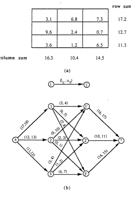
This application is concerned with consistent rounding of the elements, row sums, and column sums of a matrix, We are given a pxq matrix of real numbers D = (djJ}, with row sums axi and column sums 3j. AL our
discretion, we can round any real number c to the next smaller integer
LaJ
or to the next larger integerFoal.
The matrix rounding problem requires that we round the matrix elements, and the row and column sums of thematrix so that the sum of the rounded elements in each row equals the rounded row sum, and the sum of the rounded elements in each column equals the rounded column sum. We refer to such a rounding as a consistent rounding.
This matrix rounding problem arises is several application contexts. For example, the U.S. Census Bureau uses census information to construct millions of tables for a wide variety of purposes. By law, the bureau has an obligation to protect the source of its information and not disclose statistics that could be attributed to any particular individual. We might disguise the information in a table as follows. We round off each entry in the table, including the row and column sums, either up or down to a multiple of a constant k (for some suitable value of k), so that the entries in the table continue to add to the (rounded) row and column sums, and the overall sum of the entries in the new table adds to a rounded version of the overall sums in the original table. This Census Bureau problem is the same as the matrix rounding problem discussed earlier except that we need to round each element to a multiple of k > 1 instead of rounding it to a multiple of 1. For the moment. let us suppose that k = 1 so that this application is a matrix rounding problem in which we round any element to a nearest integer.
We shall formulate this problem and some of the subsequent applications as a problem known as the feasible flow problem. In the feasible flow problem, we wish to determine a flow x in a network G = (N, A)
satisfying the following constraints:
Xij - E xji = b(i), for i E N, (8a)
{j:(i, j)e A} (j:(j, i)e A }
0 <xij < uij, for all(i,j)e A. (8b)
As we noted in Section 2, this model includes feasible flow applications with nonzero lower bounds on arc flows since we can transform any such problem into an equivalent problem with zero lower bounds on the arc flows.
We assume that iEN b(i) = 0. We can solve the feasible flow problem by solving a maximum flow problem defined on an augmented network as follows. We introduce two new nodes, a source node s and a sink node t. For each node i with b(i) > 0, we add an arc (s, i) with capacity b(i), and for each node i with b(i) < 0, we add an arc (i, t) with capacity -b(i). We refer to the new network as the transformed network. Then we solve a maximum flow problem from node s to node t in the transformed network. It is easy to show that the problem (8) has a feasible solution if and only if the maximum flow saturates all the arcs emanating from the source node.
We show how we can discover such a rounding scheme by solving a feasible flow problem for a network with nonnegative lower bounds on arc flows. Figure 7(b) shows the maximum flow network for the matrix rounding data shown in Figure 7(a). This network contains a node i corresponding to each row i and a node j' corresponding to each column j. Observe that this network contains an arc (i, j') for each matrix element dij, an arc (s, i) for each row sum, and an arc (j', t) for each column sum. The lower and upper bounds of arc (k, I) corresponding to the matrix element, row sum, or column sum of value ct are LxaJ and
Fcx,
respectively. It is easy to establish a one-to-one correspondence between the consistent roundings of the matrix and feasible^111^
-_1_111·111
integral flows in the associated network. We know that there is a feasible integral flow since the original matrix elements induce a feasible fractional flow, and maximum flow algorithms produce all integer flows. Consequently, we can find a consistent rounding by solving a maximum flow problem with lower bounds.
column sum 16.3 10.4 row sum 17.2 12.7 11.3 14.5 (a) O
aii,
Ui L (b)Figure 7. (a) Matrix rounding problem. (b) Associated network.
The solution of a matrix rounding problem in which we round every element to a multiple of some positive integer k, as in the Census application we mentioned previously, is similar. In this case, we define the associated network as before, but now defining the lower and upper bounds for any arc with an associated real number 'cc' as the greatest multiple of k less than or equal to cc and the smallest multiple of k greater than or equal to ct. 3.1 6.8 7.3 9.6 2.4 0.7 3.6 1.2 6.5 i. --····--·- ·-II---· ... z ·Il-C^-ll---·---l-_·-··--L-YLII--l· ---· PI*--YIIP-··L·IYIIE·I
^-Application 7. Baseball Elimination Problem (Schwartz [1966])
At a particular point in the baseball season, each of n + 1 teams in the American League, which we number as 0, 1, ..., n, has played several games. Suppose that team i has won wi of the games it has already played
and that gij is the number of games that teams i and j have yet to play with each other. No game ends in a tie. An avid and optimistic fan of one of the teams, the Boston Red Sox, wishes to know if his team still has a chance to win the league title. We say that we can eliminate a specific team 0, the Red Sox, if for every possible outcome of the unplayed games, at least one team will have more wins than the Red Sox. Let wmax denote wo (i.e., the number of wins of team 0) plus the total number of games team 0 has yet to play, which, in the best of all possible worlds, is the number of victories the Red Sox can achieve. Then, we cannot eliminate team 0 if in some outcome of the remaining games to be played throughout the league, wmax is at least as large as the possible victories of every other team. We want to determine whether we can or cannot eliminate team 0.
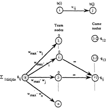
We can transform this baseball elimination problem into a feasible flow problem on a bipartite network shown in Figure 8, whose node set is N1 u N2. The node set for this network contains (i) a set N1 of n team nodes indexed 1 through n, (ii) n(n-1)/2 game nodes of the type i-j for each 1 < i < j < n, and (iii) a source node s. Each game node i-j has a demand of gij units and has two incoming arcs (i, i-j) and j, i-j) The flows on these two arcs represent the number of victories for team i and team j, respectively, among the additional gij games that these two teams have yet to play against each other (which is the required flow into the game node i-j). The flow xsi on the source arc (s, i) represents the total number of additional games that team i wins. We cannot eliminate team 0 if this network contains a feasible flow x satisfying the conditions
max > wi + xsi, for all i = 1, ... , n,
which we can rewrite as
Xsi < Wmax - wi, for all i = 1, ..., n.
This observation explains the capacities of arcs shown in the figure. We have thus shown that if the feasible flow problem shown in Figure 8 admits a feasible flow, then we cannot eliminate team 0; otherwise, we can eliminate this team and our avid fan can turn his attention to other matters.
--b(i) b(D Team Game nodes nodes nodes0 / 2 3 1 l_.~j.n gij
Figure 8. Network formulation of the baseball elimination problem. Application 8. Distributed Computing on a Two-Processor Computer (Stone [1977])
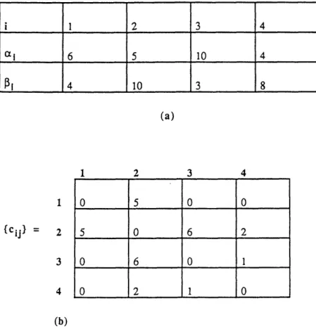
This application concerns assigning different modules (subroutines) of a program to two processors of a computer system in a way that minimizes the collective costs of interprocessor communication and computation. The two processors need not be identical. We wish to execute a large program consisting of several modules that interact with each other during the program's execution. The cost of executing each module on the two processors is known in advance and might vary from one processor to the other because of differences in the processors' memory, control, speed, and arithmetic capabilities. Let cci and Pi denote the cost of computation of module i on processors I and 2, respectively. Assigning different modules to different processors incurs relatively high overhead costs due to interprocessor communication. Let cij denote the interprocessor communication cost if modules i and j are assigned to different processors; we do not incur this cost if we assign modules i and j to the same processor. The cost structure might suggest that we allocate two modules to different processors-we need to balance this cost against the communication costs that we incur by allocating the jobs to different processors. Therefore, we wish to allocate modules of the program on the two processors so that we minimize the total processing and interprocessor communication cost.
To formulate this problem as a minimum cut problem on an undirected network, we define a source node s representing processor 1, a sink node t representing processor 2, and a node for every module of the program. For every node i, other than the source and sink nodes, we include an arc (s, i) of capacity
Pi
and an arc (i, t) of capacity cai. Finally, if module i interacts with module j during the program's execution, we include arc (i, j) with a capacity equal to cij. Figures 9 and 10 give an example of this construction. Figure 9 gives the data of this problem and Figure 10 gives the corresponding network.{Cij = 2 3 4 (b) Figure 9. Da 1 ita 2 3 4
for the distributed computing model.
Figure 10. Network for the distributed computing model.
We now observe a one-to-one correspondence between s-t cuts in the network and assignments of modules
i 1 2 3 4 ai 6 5 10 4 pi 4 10 3 8 (a) 0 5 0 0 5 0 6 2 0 6 0 1 0 2 1 0
to the two processors; moreover, the capacity of a cut equals the cost of the corresponding assignment. To establish this result, let Al and A2be an assignment of modules to processors 1 and 2 respectively. The cost of
this assignment is s ie Al ai + Fie A2 Pi + j) E AlxA2 ij. The s-t cut corresponding to thisc(i, assignment is ({s)uA1, (t)uA2). The approach we used to construct the network implies that this cut contains
an arc (i, t) of capacity ai for every i E Al, an arc (s, i) of capacity
Pi
for every i A2, and all arcs (i, j) with iE A1 and j E A2 with capacity cij. The cost of the assignment Al and A2 equals the capacity of the cut
({s)uAl, (t)uA2). (The reader might wish to verify this conclusion on the example given in Figure 10 with
A1 = (1, 2) and A2 = (3, 4).) Consequently, the minimum s-t cut in the network gives the minimum cost
assignment of the modules to the two processors.
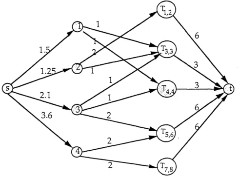
Application 9. Scheduling on Uniform Parallel Machines (Federgruen and Groenevelt [1986])
In this application, we consider the problem of scheduling a set J of jobs on M uniform parallel machines. Each job j E J has a processing requirement pj (denoting the number of machine days required to complete the job); a release date rj (representing the beginning of the day when job j becomes available for processing); and a due date dj > rj + pj (representing the beginning of the day by which the job must be completed). We assume that a machine can work on only one job at a time and that each job can be processed by at most one machine at a time. However, we allow preemptions, i.e., we can interrupt a job and process it on different machines on different days. The scheduling problem is to determine a feasible schedule that completes all jobs before their due dates or to show that no such schedule exists.
This type of preemptive scheduling problem arises in batch processing systems when each batch consists of a large number of units. The feasible scheduling problem, described in the preceding paragraph, is a fundamental problem in this situation and can be used as a subroutine for more general scheduling problems, such as the maximum lateness problem, the (weighted) minimum completion time problem, and the (weighted) maximum utilization problem.
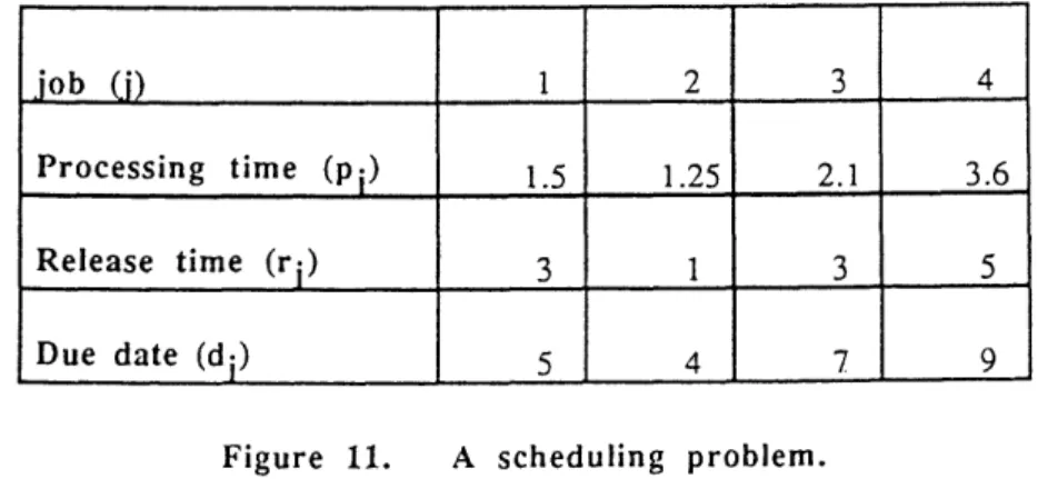
To illustrate the formulation of the feasible scheduling problem as a maximum flow problem, we use the scheduling data described in Figure 11.
Figure 11. A scheduling problem.
First, we rank all the release and due dates, rj and dj for all j, in ascending order and determine P < 2 IJI -1 mutually disjoint intervals of dates between consecutive milestones. Let Tkl denote the interval that starts at
job (i) 1 2 3 4
Processing time (pi) 1.5 1.25 2.1 3.6
Release time (r;) 3 1 3 5
the beginning of date k and ends at the beginning of date 1+1. For our example, this order of release and due dates is 1, 3, 4, 5, 7, 9. We have five intervals represented by T1,2 T3,3, T4.4 T5,6and T7,8. Notice that
within each interval Tk, the set of available jobs (that is, those released, but not yet due) does not change: we can process all jobs j with rj < k and dj > I + 1 in the interval.
We formulate the scheduling problem as a maximum flow problem on a bipartite network G as follows. We introduce a source node s, a sink node t, a node corresponding to each job j, and a node corresponding to each interval Tkl, as shown in Figure 12. We connect the source node to every job node j with an arc with capacity pj, indicating that we need to assign a minimum of pj machine days to job j. We connect each interval node Tkl to the sink node t by an arc with capacity (-k+1)M, representing the total number of machine days available on the days from k to 1. Finally, we connect job node j to every interval node TkI if rj < k and dj > 1+1 by an arc with capacity (-k+l) which represents the maximum number of machines that we can allot to job j on the days from k to 1. We next solve a maximum flow problem on this network: the scheduling problem has a feasible schedule if and only if the maximum flow value equals ,jE J pj (alternatively, for every node j, the flow on arc (s, j) is pj). The validity of this formulation is easy to establish by showing a one-to-one correspondence between feasible schedules and flows of value equal to je j pj from the source to the sink.
Figure 12. Network for scheduling uniform parallel machines. Application 10. Tanker Scheduling (Dantzig and Fulkerson [1954])
A steamship company has contracted to deliver perishable goods between several different origin-destination pairs. Since the cargo is perishable, the customers have specified precise dates (i.e., delivery dates) when the shipments must reach their destinations. (The cargoes may not arrive early or late.) The steamship company wants to determine the minimum number of ships needed to meet the delivery dates of the shiploads.
shipment is a full shipload with the characteristics shown in Figure 13(a). For example, as specified by the first row in this figure, the company must deliver one shipload available at port A and destined for port C on day 3. Figures 13(b) and 13(c) show the transit times for the shipments (including allowances for loading and unloading the ships) and the return times (without a cargo) between the ports.
(a) C D A 3 2 B 23 (b) A B C 2 1 D 1 2 (c) Figure 13. Data for the tanker scheduling problem.
We solve this problem by constructing a network shown in Figure 14(a). This network contains a node for each shipment and an arc from node i to node j if it is possible to deliver shipment j after completing shipment i; that is, the start time of shipment j is no earlier than the delivery time of shipment i plus the travel time from the destination of shipment i to the origin of shipment j. A directed path in this network corresponds to a feasible sequence of shipment pickups and deliveries. The tanker scheduling problem requires that we identify the minimum number of directed paths that will contain each node in the network on exactly one path.
(a)
Ship- Origin Destin- Delivery
ment ation date
1 Port A Port C 3
2 Port A Port C 8
3 Port B Port D 3
/ // %\, \% 'A
(b)
Figure 14. Network formulation of the tanker scheduling problem. (a) Network of feasible sequences of two consecutive shipments. (b) Maximum flow model.
We can transform this problem into the framework of the maximum flow problem as follows. We split each node i into two nodes i' and i" and add the arc (i', i"). We set the lower bound on each arc (i', i"), called the shipment arc, equal to one so that at least unit flow passes through this arc. We also add a source node s and connect it to the origin of each shipment (to represent putting a ship into service), and we add a sink node t and connect each destination node to it (to represent taking a ship out of service). We set the capacity of each arc in the network to value one. Figure 14(b) shows the resulting network for our example. In this network, each directed path from the source node s to the sink node t corresponds to a feasible schedule for a single ship. As a result, a feasible flow of value v in this network decomposes into schedules of v ships, and our problem reduces to identifying a feasible flow of minimum value. We note that the zero flow is not feasible because shipment arcs have unit lower bounds. We can solve this problem, which is known as the minimum value problem, in the following manner. We first remove lower bounds on the arcs using the transformation described in Section 2. We then establish a feasible flow in the network by solving a maximum flow problem, as described in Application 6. Although the feasible flow x satisfies all of the constraints, the amount of flow sent from node s to node t might exceed the minimum. In order to find a minimum flow, we need to return the maximum amount of flow from t to s. To do so, we find a maximum flow from node t to node s in the residual network, which is defined as follows: For each arc (ij) in the original network, the residual network contains an arc (i,j) with capacity uij - xij, and another arc (j,i) with capacity xi - li. A maximum flow between nodes t to s in the residual network corresponds to returning a maximum amount of flow from node t to node s, and provides
optimal solution of the minimum value problem.
As exemplified by this application, finding a minimum (or maximum) flow in the presence of lower bounds on arc flows typically requires solving two maximum flow problems. The solution to the first maximum flow problem is a feasible flow. The solution to the second maximum flow problem establishes a minimum (or maximum) flow.
Several other applications that bear a close resemblance to the tanker scheduling problem and are solvable using the same technique. We next briefly introduce some of these applications.
N 1%


![[DOC] Cours Liste de choix Access en Doc | Télécharger PDF](data:image/gif;base64,R0lGODlhAQABAIAAAP///wAAACH5BAEAAAAALAAAAAABAAEAAAICRAEAOw==)