Linear Conforming and Nonconforming Upwind Finite Elements for the Convection-Diffusion Equation

IMA Journal of Numerical Analysis (1988) 8, 85-103

Linear Conforming and Nonconfonning Upwind Finite Elements for the

Convection-Diffusion Equation

P H . CAUSSIGNAC AND R. TOUZANI

Departement de Mathematiques, Ecole Poly technique Federate, CH 1015 Lausanne, Switzerland

[Received 10 January 1986 and in revised form 24 June 1987] A conforming and a nonconforming method for the approximation of the stationary 2-D convection-diffusion equation at high Peclet number are pre-sented. Convergence of order h is proved in a generic case and, for a particular choice of the upwind schemes, a discrete maximum principle is established under very unrestrictive conditions on the mesh. Results of numerical computations are produced to show the practical convergence of these methods.

1. Introduction

WE consider the following steady-state convection-diffusion equation for the scalar field u.

-K Au + b-Vu + cu=f, (1.1) in a 2-D domain Q together with suitable boundary conditions; the external velocity field b, the source /, and the constants K > 0 and c s= 0 are given.

It is well known that centred finite-difference or standard finite-element approximations of the convective term in (1.1) lead to numerical instabilities or wiggles when K is small. Many upwind schemes were proposed to insure stability (see Richtmyer & Morton (1967) and Thomasset (1981) and references therein). All kinds of methods are encountered; we believe that a good one must be stable and precise enough and easy to implement, and—if possible—its convergence and a discrete version of the maximum principle should be proved.

In this paper, we construct two upwind linear triangular finite-element methods that are easy to code. We prove, in a particular case, the monotonicity of the matrix of the linear system and convergence results for simplified schemes. The upwind process is very similar to those of Hughes et al. (1979) and Brooks & Hughes (1982) for quadrilaterals. The monotonic scheme is obtained by moving quadrature points, and we should mention that—in the nonconforming case at least—the idea is due to Dervieux (see Thomasset, 1981). The local upwind coefficients are required to satisfy simple bounds in order to have the maximum principle. This is an advantage of our method over those requiring full upwinding, as for example that of Ohmori & Ushijima (1984) or some of those described in Ikeda (1983).

In Section 2, we summarize the variational formulation of the continuous problem. The approximation with the conforming element and its upwind version are given in Section 3, and monotonicity is proved in Section 4. We proceed in

the same way for the nonconforming element in Section 5 and Section 6. Convergence results are established in Section 7, whereas Section 8 is devoted to numerical results and a conclusion.

The monotonicity results of Section 4 and Section 6 are valid for particular schemes and arbitrary non-negative values of the constant c appearing in (1.1), provided that the mass matrix is (positive) diagonal. As far as the convergence estimates of Section 3 of Section 7 are concerned, we have to assume c > 0; since the standard schemes converge for large K or small mesh size h, our results are stated for values of ic/h that are small beside the maximum of the velocity modulus.

2. Summary of the continuous problem

We assume, for simplicity, that the open bounded domain £2c[R2 with boundary F is polygonal. As usual, L2(£2) will denote the space of square-integrable functions on Q, equipped with the norm ||#||o,«, and Hj(i2) the Sobolev space of functions vanishing on F which, together with their first-order derivatives, are in \}{Q). The norm on Hj(£2) can be chosen as \u\ia = ||V«||0,fl; the velocity is assumed to have continuous first-order partial derivatives, that is, b 6 C1^)2. Using the notation (•, •) for the inner product of L2(£2) and the one of L\Q)2 as well, we define the bilinear form

a(u, V) = K{VU, Vv) + (b • Vu, v) +c(u, v), K>0, CS=0. (2.1)

A weak variational formulation of the problem corresponding to equation (1.1) with homogeneous Dirichlet boundary conditions reads:

Find u e HS(0) such that a(u, v) = (f,v)Vve Hl(Q). (2.2) Integrating equation (2.1) by parts yields the coercivity of a(m, •), provided that

div b is small enough. Without loss of generality, we assume from now on that div6(x) = 0 (xeQ), (2.3) and shall make later some comments on the case where this condition is not met. Existence, uniqueness, and a weak form of the maximum principle are sum-marized in the following lemma.

LEMMA 2.1 For f eL2(Q), Problem (2.2) has one and only one solution u.

Furthermore, iff^O, one has u^O.

Proof. Existence and uniqueness follow from the Lax-Milgram theorem. For the maximum principle, see Gilbarg & Trudinger (1977: Thm 8.1). D

Remark. The cases of inhomogeneous Dirichlet or mixed Dirichlet-Neumann boundary conditions can be reduced to the formulation (2.2) by putting the inhomogeneity in the right-hand side. Similarly, the pure Neumann problem can be solved, provided that a compatibility condition is added.

LINEAR CONFORMING AND NONCONFORMING UPWIND FINITE ELEMENTS 8 7 3. Linear conforming approximation

Let Th be an admissible triangular mesh of Q (h denotes the largest side);

recall that a family {Th}h of admissible triangulations is regular if the smallest

angle 9h remains bounded from below, i.e. dh~sz 60>0, as h goes to zero (see

Temam, 1984: pp. 73-74). We define the sets

yh = {S e Q : 5 is a vertex of a triangle K e Th}, (3.1)

Sft = {SeSfh:Str}, (3.2)

ZK = SfhnK {KeTh), (3.3)

JfK(S) = SK\{S} (KeTh,SeIK), (3.4)

and finite-dimensional vector spaces

Vh = {ve C°(£?) : v \K is a linear polynomial V KeTh}, (3.5)

V0h = {veVh:v{S) = OVSeSrhnr}. (3.6)

The standard Prapproximation of Problem (2.2) is then given by:

Find uh e VOh such that a(uh, vh) = (/, vh)Vvhe VOh. (3.7)

Since the space VOh <= Hj(£2) is complete, we have the following result.

LEMMA 3.1 / / / e L2(f3), then Problem (3.7) has one and only one solution uh.

At very low values of the diffusion coefficient K, stability and convergence results for uh in the Hj norm are not interesting, since the constants in the

estimates are proportional to if"1. Uniform estimates can be obtained in the norm

as quoted in the following lemma.

LEMMA 3.2 We assume that the solution u of (2.2) is in H2(Q). Then, for c > 0

and K =£ K0 < oo, there exist positive constants Cx and C2, independent of h and K,

such that

ll«*llr«C1|[/||o.0, (3.9)

\\u-uh\\K^C2h\u\2,a, (3.10)

where |»|2,a is the usual seminorm of the Sobolev space H2(£2).

Proof. Noticing that a(u, u) = \\u\\2K, we see that the bound (3.9) follows directly

from (3.7) and the Cauchy-Schwarz inequality. The error estimate (3.10) is obtained by a standard reasoning (see for example Ciarlet, 1978: Thm 3.2.2) combined with:

|«(M,u)|«C||u||r|i;|I.f l. •

Let us now introduce the general form of the upwind approximation. First, we decompose the velocity at each vertex as

To obtain the upwind scheme, we replace the convective term in (2.1) by

KeTh

b

(u,v)= 2 I T 2 U[v(S)b(S)- Vu\K-u(S)b(S)-Vv\K]

(u,veVh), (3.12)

where \K\ is the area of the triangle K. The local upwind parameters a§s. are

such that

o&.fl&.sOand|a&.|«i ( X e T ^ ^ S ' e ^ ) , (3.13) and the upwind vectors ff£5. satisfy

|o&.|«CA (KeTh;S,S'eIK), (3.14)

where C > 0 is independent of K,S,S', and jr. By defining

ah(u,v) = K(Vu,Vv) + bh{u,v) + c{u,v) (/c>0, c3=0), (3.15)

the upwind approximation of Problem (2.2) reads

Find uh e VOh such that ah(uh, vh) = (f, vh)Vvhe VOh. (3.16)

The coercivity of ah(m, •) implies the existence and uniqueness of the solution uh

of this problem.

EXAMPLES. If we set

a^.^S^ (KeTh;S,S'eIK), (3.17)

and use the linearity of the functions in Vh, the formula (3.12) can be written as

- uh(S - a&iS' - S))B%sSSr- Vvh

which shows that the standard numerical integration of the convective term with quadrature points at 5 e £K is replaced by a formula with 'upwind' points at

5 ± a r £ ; . ( 5 ' - 5 ) . This scheme is analogous to that of Hughes et al. (1979) for quadrilaterals in which only one displaced quadrature point is used. The next schemes correspond to that of Brooks & Hughes (1982), which is obtained by an argument based on the concept of artificial diffusivity. The first one is defined by

o ^ = 6(5)|55r|/|A(5)| (KeTh;S,S'eZK) (3.18)

or

o&. = b{S)h/\b{s)\ (KeTh;S,S'eIK), (3.18')

and the second one by

a^s. = bK\SSr\/\bK\ (KeTh;S,S'eIK) (3.19)

or

LINEAR CONFORMING AND NONCONFORMING UPWIND FINITE ELEMENTS 8 9

where bK is a mean value over K, for example:

The advantage of the schemes (3.18) to (3.19') is their lack of diffusivity in the direction perpendicular to the velocity or mean velocity.

4. Maximum principle for the scheme (3.17)

We denote the Lagrangian basis of Vh by {0s}SeSr,, and introduce the operator R : US2-* U2 of rotation by angle - |JI:

x2) = (x2,-x1). (4.1)

A triangulation will be said to be of an acute type if no angle greater than |JI occurs. We set A^ = dimVA and N0 = dim VOh, and shall sometimes use a

numbering of the vertices such that

In order to prove properties of the matrix A, with entries

A^a^s^s) (l«iJ«A0, (4.2) which lead to the maximum principle, some restrictions on the upwind param-eters are necessary.

HYPOTHESIS 4.1 V K e Th, V S e IK, V S',S" e JfK(S), and if B$s. * 0:

Remark. If the mesh is made of equilateral triangles, then the condition (4.3) reads

where the local P6clet numbers are given by PKss=\\B^s.\h2lK.

(The usual mesh P6clet number is defined as Pe = |6| h/ic.)

We are ready to establish the properties of the matrix A, in the case c — 0.

LEMMA 4.2 Assuming that Hypothesis 4.1 holds and that the triangulation is of an

acute type, one has, for the scheme (3.17) and c = 0:

(1) E^// = 0 (l^^AO,

(2) As>0 (l*i*N),

Proof. (1) It is easily seen that each term contributing to Ay contains V(j>Sj. The

assertion then follows since T^jLi 4>s, =

1-(2) This is a consequence of the coercivity of ah(», •).

(3) On the triangle K whose vertices are S,S',S", with positive oriented boundary, we have

by using (3.11), (3.12), (3.15), (3.17), and the linearity of the basis functions, the contribution of K to ah(<pS', (j>s) can be written as

Let us show that af, the first expression in large parentheses, is «0. If Bss1 ^ 0,

then B$s.(l - 2 a r ^s. ) ^ 0 since 5&>ar&. 2=0, and af « 0 because the triangulation is of acute type. Otherwise, if B$S' > 0 , then af =£0 by inequality (4.3). A similar

reasoning allows to show that a* =s 0. •

Let us recall that a matrix is monotonic if its inverse exists and is positive. The next proposition states that the matrix A of the linear system, with entries

( U i , / s / V0) , (4.4) is monotonic.

PROPOSITION 4.3 Assume that the triangulation is of an acute type, Hypothesis 4.1 holds, and the mass matrix is diagonal with positive diagonal entries. If furthermore, there exists an element KeTh and vertices SeHKC\r and S'e

JfK(S) n Sf°h such that either

(a) Bss- = 0 and the angle of K at S is less than \n or

(b) B$s>0,

then the matrix A for the scheme (3.17) is monotonic. Proof. By Lemma 4.2, we have

(1) f U ^ O (l*i*N

),

Now, in order to prove that A is monotonic, it is sufficient (Berman & Plemmons, 1979: Theorem 2.3) to show that EfiiAioj>0, for some /oe {1, 2, . . . , No}. It

LINEAR CONFORMING AND NONCONFORMING UPWIND FINITE ELEMENTS 9 1

satisfied, then ah(<t>s, <ps) < 0 . Hence, there exists an entry of A, not belonging to

A, which is negative. Since Yis-e9ii,Qh((i>s-> <Ps) = ®> we have the desired

property. •

The condition on the mass matrix occurring in the hypotheses of Proposition 4.3 can be achieved by numerical integration with quadrature points at the vertices. We now state the maximum principle and a stability property.

COROLLARY 4.4 Assume that the hypotheses of Proposition 4.3 hold, f e L2(£2), and the mass matrix is diagonal with positive diagonal entries if c > 0. Then, Problem (3.15) with the scheme (3.17) has one and only one solution uh such that

uh5s0 iff 3= 0. Furthermore, if c>0 and f e V°(Q), there exists a constant C> 0,

independent of h and K, such that ||«alU=£C||/||«>, where \\*\\ao is the usual norm

Proof. The first part of the assertion is a direct consequence of Proposition 4.3. To prove the stability property, it suffices to show that the induced €™ norm of A "1 is independent of K. For c > 0 , we have A=A + M, with, V i e

jJ^/y^O, M,j = m,bii (1 =£;=£ No), m,>0:

The vector z e i "0 with components z, = (min, m,)"1 (l^y^No) satisfies Sfi, Avzj =M (1«i «No); therefore ||A-'|L = ||z|U = C. •

Remark. If div 6 ^ 0 , one has to replace (3.12) and (3.13) by

b

(u,v)= E ^ S Us)b(s)-Vu\K

« E 9

.

if Bss' >0 . For a mesh made of equilateral triangles, (4.7) reads aKss^\-\lPKss; P£->0,

with

P& = lB$s.h2/K.

The case of equality corresponds to the recommended choice of Hughes et al. (1979). On the other hand, one can show that the standard approximation leads to a monotonic matrix if P$s. < 1. Hence, a natural choice of the upwind

parameters is, in this case,

K = f0 i f P & . < l , ass' 11-1/P&. otherwise.

5. The linear nonconforming approximation

The nonconforming element presented here can be easily generalized to the 'Pj — Po' finite element for solving Navier-Stokes equations (Thomasset, 1981). We consider again an admissible triangulation Th of Q and define the sets

Mh = {M e Q : M is the midpoint of a side of a triangle K e th}, (5.1)

M°h = {MeMh:M$r}, (5.2)

MK = MhC\K (KeTh), (5.3)

•yr*(AO = M*\{M}, (MeMh) (5.4)

and finite-dimensional vector spaces

V'h = {v e L2(£2) : u \K is a linear polynomial V K e Th; v is

continuous at each point W e i J } ,

I / ; = { u e y i : t ) ( M ) = O V i W € l , n r } . (5.6) Since the space Voh is an external approximation of Hl(£2), we must define the

bilinear form as follows.

ah(u, v)= 2 [K(Vu,Vv)K + k((b-Vu,v)K-(b-Vv,u)K)] + c(u,v),

Hex*

K>Q, c5=0, (5.7) where (•, »)K is the inner product of L2(K) or L\K)2.

Let us introduce the seminorm

(5.8) and the norm j

,/. = ( z « " , ">* + <Vu, Vi/)*)) . (5.9) The nonconforming approximation of Problem (2.2) at zero-divergence velocity then reads:

Find uh e V'Oh such that dh(uh, vh) = {f,vh) V vh e V'Oh. (5.10)

As in the continuous case, we have the following discrete Poincare' inequality.

LEMMA 5.1. / / Th belongs to a regular family of triangulations, then there exists a

constant C(£2)>0 such that

i/*|U VvheVOh, (5.11)

LINEAR CONFORMING AND NONCONFORMING UPWIND FINITE ELEMENTS 9 3

Proof. See Temam (1984: Propn4.13). •

It follows from (5.7) that the bilinear form aA(«, •) is coercive on V'Qh and

hence we have the following result.

LEMMA 5.2. If f eL2(£2), the problem (5.10) has one and only one solution

uh. a

In the norm:

ll«llr.* = (*ll«ll* + c|N|g,o)4, K>0, c>0, (5.12) the form a'h{*, •) is also coercive, and the Cauchy-Schwarz inequality gives us the

stability result

s£C,|lf||o,0, (5.13) where Cx > 0 is independent of h and tc.

To set up the nonconforming upwind approximation, we first decompose the velocity at the mid-side nodes as follows:

b{M)= 2 B%M.MM' (MeMh,KeTh), (5.14)

M'eJfK(M)

and require the upwind coefficients and vectors to satisfy

« i (KeTh;M,M'eMK), (5.15)

'\ (KeTh;M,M'eMK), (5.16)

where C>0 is independent of K, M, M', and K.

As in the conforming case, we introduce the upwind forms

b'h(u, v) = 2 ^ f 2 (\{v{M)b{M) -Vu\K- u(M)b(M) • Vv\K)

(u,veV'h)

2

M'eXtK(M)

(5.17) a'h(u, v)= 2J K(VU, Vv)K + b'h(u, v) + c(u, v), K>0, C5=0, (5.18)

and the upwind approximate problem reads:

Find uh e V'Oh such that a'h{uh, vh) ={f,vh) V«f te V'Oh. (5.19)

Obviously, this problem has a unique solution. The schemes analogous to (3.17) and (3.18) are

V (KeTh;M,M'eMK), (5.20)

<tiM. = b(M)\MMr\/\b{M)\ (KeTh;M,M'eMK), (5.21)

6. Maximum principle for the scheme (5.20)

We set TV = dim V'h and No = dim V'Oh and assume that the mid-side nodes are

numbered so that Ml = {Mu M2,.. •, MNo}.

Let A' be the matrix with entries

l (6.1)

where {<f>M)fLi is the usual Lagrangian basis of V'h.

We make the following assumption.

HYPOTHESIS 6.1 V K e Th, V M e MK, V M',M" e Jf'K(M), and if BKMM. ¥= 0:

12* R(WMr)-R(MMr)

^jr-, 7J772 . (6-2)

\t>MAf\ 1^1

where R is defined by (4.1).

If the mesh is made of equilateral triangles, the last condition reads:

where the local P£clet numbers are given by:

One can copy the proof of Lemma 4.2 to obtain a similar lemma, leading to the monotonicity of the matrix A', with entries

i (l*i,j*£N0). (6.3)

Note that, here, the exact mass matrix is diagonal with positive diagonal entries.

PROPOSITION 6.2 Assume that the triangulation is of acute type, Hypothesis 6.1 holds, and there exist KeXh, MeMKnr, and M' e N'K(M)C\M°h such that

either

(a) BMM' = 0 and the angle at the vertex opposite to M' in K is less than %K

or

(b) BKM-M>Q.

Then the matrix A' for the scheme (5.20) is monotonic and T,f=\A'ij^Q (lssf as

No).

Proof. The proof is similar to that of Proposition (4.3); here, we have

on triangle K with mid-side nodes M,M',M" and positive-oriented boundary. D The reasoning leading to the conclusion of Corollary 4.4 applies here too, and gives the maximum principle and stability.

COROLLARY 6.3 Assume that the hypotheses of Proposition 6.2 hold and

/ e L2( f l ) . Then, Problem (5.19) with the scheme (5.20) has one and only one solution uh which satisfies

LINEAR CONFORMING AND NONCONFORMING UPWIND FINITE ELEMENTS 9 5

Furthermore, if c > 0 and / e L°°(£2), then there exists C > 0 , independent of h and K, such that

max K(M,)|«C|1/|U. •

Remark. So far, we have given the nonconforming scheme for zero-divergence velocity. If 6\\ b ^ 0 , we replace (5.17) and (5.15) by

¥r 2 (v(M)b(M)-Vu\K

(u,veV'

), (6.4)

^ l , «$,„• = 0 ifBJU- = O. (6.5) The condition (6.2) becomes

12A: R(M"M')-R(MM") „ , , ,x

^

£

J

U

>

0 (6.6)

7. Convergence results

Throughout this section, we shall assume the solution u of the continuous problem (2.2) to be in H2(i2) and set

B = max |6(JC)| . (7.1)

Our schemes belong to the family of methods which consist in adding an artificial diffusive term of order h to the bilinear form of the continuous problem. Such a method improves the stability but not the convergence, and we expect to have uniform estimates of the same order as for the standard scheme. The simplest upwind technique of this kind is defined by adding h{Vu, Vu) to the bilinear form a(«, •) (equation (2.1)); this procedure, unlike our schemes, ignores the local features of the flow described by the velocity b.

The contribution of an element K to the artificial diffusion in (3.12) can be written as follows.

^ Vv \K)

where the matrix function AK is positive semidefinite and all its entries are

bounded by

|A*(S)| < Ch(S e I

),

the bilinear form (3.15) as the result of numerical integration applied to

ah(u, v) = K{VU,VV) + {b-Vu,v) +c{u,v)+~ £ ( A / | ^ , | ^ ) . (7-3)

2 ,-.y=i \ OX; dXjl

We shall prove hereafter convergence and stability for the solution of the discrete problem:

Find uh e VOh such that ah{uh, vh)=(f,vh) Vvhe VOh. (7.4)

Notice that existence and uniqueness are ensured, provided that / e L2(Q) and

the matrix A is positive semidefinite almost everywhere on Q. This last property implies also that the equation

\\u\\K,h = ah(u,u)l (7.5)

defines a norm on H^(£2).

Denoting by Wla>(i2) the Sobolev space of functions which are, together with their first-order derivatives, in L°°(£2), we give some technical results in the next lemma.

LEMMA 7.1 Assume that c>0, K<{Bh, A ^ W ' ^ Q ) (i,j = 1,2), the W1-" norm of these functions is bounded uniformly in h and K, and the matrix A is symmetric positive semidefinite almost everywhere on Q. Then, one has

(1) I M I O , O * C , | | M | U forueHl0{Q),

(2) ||«IU,/1^C2|u|1,fi forueHl(Q), (3) \ah(u,v)\^C3\u\lia\\v\\Kih foru.veHl

(4) \ah(u,wh)-(f,wh)\^C4h\u\2,a\\wh\\h forwheV0h,

if ue H2(£2) is the solution of the continuous problem (2.2).

Proof. Properties (1) and (2) are direct consequences of Definition (7.5) and the Poincar6 inequality.

(3) From (7.3), one gets

)u dv

The first two terms in the right-hand side are easily bounded by

the latter inequality coming from Property (1). It remains to estimate the last term. Since the matrix with entries aVj = Kbit + ^BhAjj is positive definite, one can

use the Cauchy-Schwarz inequality, which yields

K,h-LINEAR CONFORMING AND NONCONFORMING UPWIND FINITE ELEMENTS 9 7

(4) Equations (2.1), (2.2), (7.3), (7.4), and an integration by parts yield Bh

~2 „

^ Ch \u\2a IKHo.c^ CCxh \u\2a \\wh\\h (wheVOh). D

The convergence is stated in the following theorem.

THEOREM 7.2 / / the solution u of Problem (2.2) is in H2(i2), with f e \?{Q), and c >0, and the hypotheses of Lemma 1.1 hold, then there exists a constant C>0, independent of h and K, such that

\\u-uh\\K,h^Ch\u\2,a, (7.6)

where uh is the solution of Problem (7.4).

Proof. Using Parts (2) and (3) of Lemma 7.1, instead of the continuity of the form ah(', •) in the norm ||»|U,*, one can obtain, by a technique similar to the

proof of the second Strang lemma,

I || ^ / - / • * . I , ,~n(u, Wh) - {f, Wh)\\

«-«*U.*«C( mf \u-v

\

+ sup — I.

WVO* H*6Vm \\Wh\\h /

The assertion follows by choosing vh as the interpolate of u and applying Part (4)

of Lemma 7.1. •

Remarks. (1) Assume that the functions Atj are only in L°°(£2). Since the matrix

A is positive semidefinite, we may write Bh

2

du dwh

du

This means that we have, in place of (7.6),

12 . o . ( 7 . 7 )

Notice that the scheme defined by (3.12) satisfies the preceding assumption because the functions A/y can be obtained by linear interpolation of the nodal values on each triangle. To achieve the proof of the bound (7.7) for our conforming scheme, we have only to estimate the error due to numerical integration of the convective term. The technique is standard (see Ciarlet, 1978: §4.1) and requires a slightly modified version of the first Strang lemma. The key estimate is given by

(2) For the nonconforming scheme defined by equations (5.17)—(5.18), we introduce, in place of (7.3), the form

'kiu, v) =

U(Vu, Vv)

₊

Bh

( 7-8 )

with the functions A* defined from (5.17) by linear interpolation as indicated above. An estimate like (7.7), for c>0, K<\Bh, and a mesh Th belonging to a

regular family of triangulations, is valid in this case too, in the norm

Huli;.fc = fl;(H,«)i. (7.9) Actually, denoting by u e H2(£2) the solution of the continuous problem (2.2), integration by parts yields

2 f du . v f — whds + \ 2J J3K on KeT J3 n ds + •Bh

2

2

The first two absolute values in the right-hand side can be bounded, in a way analogous to the proof of Theorem 3 in Crouzeix & Raviart (1973), by

ChK~l\u\2,K\\wh\\Kih,

and similarly for the last term, since A*eLT(K). The numerical integration in (5.17), exact for polynomials of degree 2, does not affect the convergence estimate.

(3) If the mesh contains equilateral triangles only, then the coefficients A,y corresponding to the scheme (3.18') are in W1:o(i2), and the conclusion of Theorem 7.2 holds.

8. Numerical results and conclusion

We have performed two tests in order to show the practical convergence of the schemes presented in this paper.

For the first test, the domain is the unit square Q = (0,1) X (0,1). We solved equation (1.1), with b = (1,0), / = 0, c = 0, K = 10~3, and the boundary conditions

u(0, y) = \ and u(\,y) = 0 (0=£.y=sl),

The exact solution is given by

LINEAR CONFORMING AND NONCONFORMING UPWIND FINITE ELEMENTS 2.00-1 1.60- 1.20- 0.80- 0.40-99 0.00 0.00 0.20 0.40 0.60 0.80 1.00

FIG. 1. Profiles of the solution along y = 3. E: exact solution, C: centred scheme, • : conforming upwind scheme, [x]: nonconforming upwind scheme.

In Fig. 1, we present the profiles in the section y = 5 of the exact solution, the standard conforming approximation, the upwind conforming approximation with the scheme (3.17), and the upwind nonconforming approximation with the scheme (5.20). The mesh consists of identical squares halved by parallel diagonals; we have 550 triangles with 256 nodes in the conforming case and 200 triangles with 320 nodes in the nonconforming one.

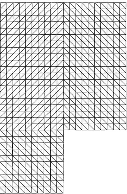
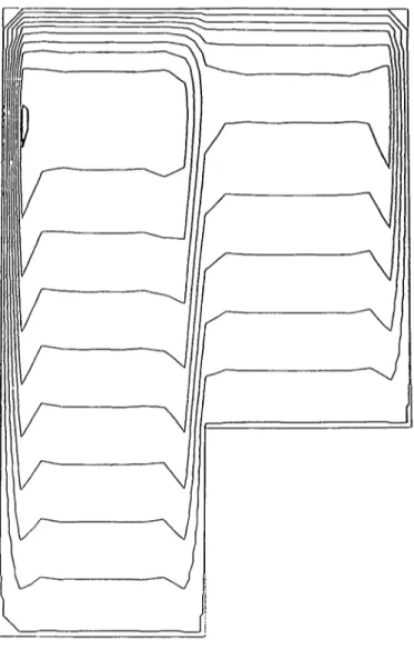
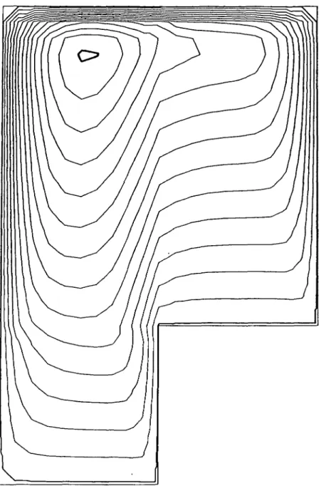
For the second test, the domain and its triangulation are given by Fig. 2. The velocity is b - (0, 1), the external source is / = 1 and c = 0; the diffusion coefficient is K = 10~3, and we impose the boundary condition u\dQ = 0. This problem is very difficult to solve, since there are boundary layers on 9Q at x = 0, x = 2, and y = 3 and a transition layer at x = 1 for Ky < 3. Outside the layers, the exact solution can be approximated by the linear functions u=.y for 0 < ; t < l and u = y — 1 for 1< x < 2. The isolines for the upwind conforming schemes (3.17) and (3.18) can be found respectively in Fig. 3 and Fig. 4. As expected, the latter scheme is less diffusive than the former one.

Note that, for both tests, the upwind coefficients were calculated as if the triangulation were equilateral, by using the equals sign in inequalities (4.3) or (6.2).

The conforming and nonconforming upwind finite elements we have presented here satisfy, in a particular case, the monotonicity property. Results lacking uniform convergence, like those of Lemma 7.1, can be found in the literature (Ohmori & Ushijima (1984), Ikeda (1983)). Except for a special case, we have only proved a uniform convergence of order htc'* in the norm \\*\\K,h defined by

\ \ \

\ \ \ \

\ \ \

\ \

FIG. 2. The domain with its triangulation (1(XX) triangles, 551 nodes). The lower left corner has the coordinates x = 0, y = 0.

(7.3) and (7.5); this implies a convergence rate of order hK'1 in the norm ||»||1>Q. Usually, convergence is discussed on the formulation without numerical integra-tion (see Johnson et al., 1984), for which we have an O(h) estimate for the conforming scheme in the \\»\\K_h norm; this means that the upwind process does

LINEAR CONFORMING AND NONCONFORMING UPWIND FINITE ELEMENTS 101

FIG. 3. Isolines of the solution for the upwind scheme (3.17). (15 equidistant isolines from 0 to 2.4).

the three-dimensional case and/or to incompressible Navier-Stokes equations is quite obvious.

Acknowledgement

FIG. 4. Isolines of the solution for the upwind scheme (3.18). (Same values as Fig. 3.)

REFERENCES

BERMAN, A., & PLEMMONS, R. J. 1979 Nonnegative Matrices in the Mathematical Sciences, New-York: Academic Press.

BROOKS, A. N., & HUGHES, T. J. R. 1982 Streamline-upwind Petrov-Galerkin formulations for convective dominant flows with particular emphasis on the

incom-LINEAR CONFORMING AND NONCONFORMING UPWIND FINITE ELEMENTS 103

pressible Navier-Stokes equations. Comput. Methods Appl. Mech. Engng. 32, 199-259.

CIARLET, P. G. 1978 The Finite Element Method for Elliptic Problems. Amsterdam: North-Holland.

CROUZEIX, M., & RAVIART, P. A. (1973) Conforming and nonconforming finite element methods for solving the stationary Stokes equations I. RAIRO Anal. Numer. 3, 33-76.

GILBARG, D., & TRUDINGER, N. 1977 Elliptic Partial Differential Equations of Second Order. Grundlehren der mathematischen Wissenschaften 224. Berlin: Springer.

HUGHES, J. T. R., LIU, W. K., & BROOKS, A. N. 1979 Review of finite element analysis of incompressible viscous flow by the penalty function formulation. / . Comp. Phys. 30, 1-40.

IKEDA, T. 1983 Maximum Principle in Finite Element Models for Convection-Diffusion Phenomena. Lecture Notes in Numerical and Applied Analysis Vol. 4. Amsterdam: North-Holland.

JOHNSON, C , NAVERT, V., & PITKARANTA, I. 1984 Finite element method for linear hyperbolic problems. Comput. Methods Appl. Mech. Engng. 45, 285-312.

OHMORI, K., & USHIJIMA, T. 1984 A technique of upstream type applied to a linear conforming finite element approximation of convective diffusion equations. RAIRO Anal. Numer. 18, 309-332.

RICHTMYER, R. D., and MORTON, K. W. 1967 Difference Methods for Initial Value Problems. New York: Interscience.

TEMAM, R. 1984 Navier-Stokes Equations (revised edn) Amsterdam: North-Holland. THOMASSET, F. 1981 Implementation of Finite Element Methods for Navier-Stokes