Publisher’s version / Version de l'éditeur: Computer Science, 2017-08-11
READ THESE TERMS AND CONDITIONS CAREFULLY BEFORE USING THIS WEBSITE. https://nrc-publications.canada.ca/eng/copyright
Vous avez des questions? Nous pouvons vous aider. Pour communiquer directement avec un auteur, consultez la première page de la revue dans laquelle son article a été publié afin de trouver ses coordonnées. Si vous n’arrivez pas à les repérer, communiquez avec nous à [email protected].
Questions? Contact the NRC Publications Archive team at
[email protected]. If you wish to email the authors directly, please see the first page of the publication for their contact information.
NRC Publications Archive
Archives des publications du CNRC
This publication could be one of several versions: author’s original, accepted manuscript or the publisher’s version. / La version de cette publication peut être l’une des suivantes : la version prépublication de l’auteur, la version acceptée du manuscrit ou la version de l’éditeur.
Access and use of this website and the material on it are subject to the Terms and Conditions set forth at
Emotion intensities in tweets
Mohammad, Saif M.; Bravo-Marquez, Felipe
https://publications-cnrc.canada.ca/fra/droits
L’accès à ce site Web et l’utilisation de son contenu sont assujettis aux conditions présentées dans le site LISEZ CES CONDITIONS ATTENTIVEMENT AVANT D’UTILISER CE SITE WEB.
NRC Publications Record / Notice d'Archives des publications de CNRC: https://nrc-publications.canada.ca/eng/view/object/?id=ce218860-e351-49fc-8443-f227d219fe59 https://publications-cnrc.canada.ca/fra/voir/objet/?id=ce218860-e351-49fc-8443-f227d219fe59
Emotion Intensities in Tweets
Saif M. Mohammad
Information and Communications Technologies National Research Council Canada
Ottawa, Canada
Felipe Bravo-Marquez Department of Computer Science
The University of Waikato Hamilton, New Zealand [email protected]
Abstract
This paper examines the task of detecting intensity of emotion from text. We cre-ate the first datasets of tweets annotcre-ated for anger, fear, joy, and sadness intensities. We use a technique called best–worst scal-ing (BWS) that improves annotation con-sistency and obtains reliable fine-grained scores. We show that emotion-word hash-tags often impact emotion intensity, usu-ally conveying a more intense emotion. Fi-nally, we create a benchmark regression system and conduct experiments to deter-mine: which features are useful for detect-ing emotion intensity; and, the extent to which two emotions are similar in terms of how they manifest in language.
1 Introduction
We use language to communicate not only the emotion we are feeling but also the intensity of the emotion. For example, our utterances can con-vey that we are very angry, slightly sad, absolutely elated, etc. Here, intensity refers to the degree or amount of an emotion such as anger or sad-ness.1 Natural language applications can benefit from knowing both the class of emotion and its intensity. For example, a commercial customer satisfaction system would prefer to focus first on instances of significant frustration or anger, as op-posed to instances of minor inconvenience. How-ever, most work on automatic emotion detection has focused on categorical classification (presence of anger, joy, sadness, etc.). A notable obstacle in developing automatic affect intensity systems is the lack of suitable annotated data. Existing af-fect datasets are predominantly categorical.
Anno-1
Intensity is different from arousal, which refers to the extent to which an emotion is calming or exciting.
tating instances for degrees of affect is a substan-tially more difficult undertaking: respondents are presented with greater cognitive load and it is par-ticularly hard to ensure consistency (both across responses by different annotators and within the responses produced by an individual annotator).
Best–Worst Scaling (BWS) is an annotation scheme that addresses these limitations (Louviere,
1991;Louviere et al.,2015;Kiritchenko and Mo-hammad, 2016, 2017). Annotators are given n items (an n-tuple, where n > 1 and commonly n = 4). They are asked which item is the best (highest in terms of the property of inter-est) and which is the worst (lowest in terms of the property of interest). When working on 4-tuples, best–worst annotations are particularly ef-ficient because each best and worst annotation will reveal the order of five of the six item pairs. For example, for a 4-tuple with items A, B, C, and D, if A is the best, and D is the worst, then A > B, A >C, A > D, B > D, and C > D.
BWS annotations for a set of 4-tuples can be easily converted into real-valued scores of associ-ation between the items and the property of inter-est (Orme,2009;Flynn and Marley,2014). It has been empirically shown that annotations for 2N 4-tuples is sufficient for obtaining reliable scores (where N is the number of items) (Louviere,1991;
Kiritchenko and Mohammad, 2016).2 The lit-tle work using BWS in computational linguistics has focused on words (Jurgens et al., 2012; Kir-itchenko and Mohammad, 2016). It is unclear whether the approach can be scaled up to larger textual units such as sentences.
Twitter has a large and diverse user base, which entails rich textual content, including non-standard language such as emoticons, emojis,
cre-2
At its limit, when n = 2, BWS becomes a paired
com-parison (Thurstone, 1927;David, 1963), but then a much larger set of tuples need to be annotated (closer to N2).
atively spelled words (happee), and hashtagged words (#luvumom). Tweets are often used to con-vey one’s emotions, opinions towards products, and stance over issues. Thus, automatically de-tecting emotion intensities in tweets has many ap-plications, including: tracking brand and product perception, tracking support for issues and poli-cies, tracking public health and well-being, and disaster/crisis management.
In this paper, we present work on detecting intensities (or degrees) of emotion in tweets. Specifically, given a tweet and an emotion X, the goal is to determine the intensity or degree of emotion X felt by the speaker—a real-valued score between 0 and 1.3 A score of 1 means that the speaker feels the highest amount of emotion X. A score of 0 means that the speaker feels the lowest amount of emotion X. We annotate a dataset of tweets for intensity of emotion using best–worst scaling and crowdsourcing. The main contributions of this work are summarized below: • We formulate and develop the task of detecting
emotion intensities in tweets.
• We create four datasets of tweets annotated for intensity of anger, joy, sadness, and fear, respectively. These are the first of their kind.4 • We show that Best–Worst Scaling can be
suc-cessfully applied for annotating sentences (and not just words). We hope that this will encour-age the use of BWS more widely, producing more reliable natural language annotations. • We annotate both tweets and a hashtag-removed
version of the tweets. We analyse the impact of hashtags on emotion intensity.
• We create a regression system, AffectiveTweets Package, to automatically determine emotion intensity.5 We show the extent to which various features help determine emotion intensity. The system is released as an open-source package for the Weka workbench.
• We conduct experiments to show the extent to which two emotions are similar as per their manifestation in language, by showing how predictive the features for one emotion are of another emotion’s intensity.
3Identifying intensity of emotion evoked in the reader, or
intensity of emotion felt by an entity mentioned in the tweet, are also useful, and left for future work.
4
We have also begun work on creating similar datasets annotated for other emotion categories. We are also creating a dataset annotated for valence, arousal, and dominance.
5
https://github.com/felipebravom/AffectiveTweets
• We provide data for a new shared task WASSA-2017 Shared Task on Emotion Intensity.6 The competition is organized on a CodaLab website, where participants can upload their submis-sions, and the leaderboard reports the results.7 Twenty-two teams participated. A description of the task, details of participating systems, and results are available in Mohammad and Bravo-Marquez(2017).8
All of the data, annotation questionnaires, evalua-tion scripts, regression code, and interactive visu-alizations of the data are made freely available on the shared task website.6
2 Related Work
Psychologists have argued that some emotions are more basic than others (Ekman, 1992; Plutchik,
1980;Parrot,2001;Frijda, 1988). However, they disagree on which emotions (and how many) should be classified as basic emotions—some pro-pose 6, some 8, some 20, and so on. Thus, most ef-forts in automatic emotion detection have focused on a handful of emotions, especially since manu-ally annotating text for a large number of emotions is arduous. Apart from these categorical models of emotions, certain dimensional models of emotion have also been proposed. The most popular among them, Russell’s circumplex model, asserts that all emotions are made up of two core dimensions: va-lence and arousal (Russell, 2003). In this paper, we describe work on four emotions that are the most common amongst the many proposals for ba-sic emotions: anger, fear, joy, and sadness. How-ever, we have also begun work on other affect cat-egories, as well as on valence and arousal.
The vast majority of emotion annotation work provides discrete binary labels to the text instances (joy–nojoy, fear–nofear, and so on) (Alm et al.,
2005;Aman and Szpakowicz,2007;Brooks et al.,
2013; Neviarouskaya et al., 2009; Bollen et al.,
2009). The only annotation effort that provided scores for degree of emotion is byStrapparava and Mihalcea (2007) as part of one of the SemEval-2007 shared task. Annotators were given newspa-per headlines and asked to provide scores between
6
http://saifmohammad.com/WebPages/EmotionIntensity-SharedTask.html
7
https://competitions.codalab.org/competitions/16380
8Even though the 2017 WASSA shared task has
con-cluded, the CodaLab competition website is kept open. Thus the best results obtained by any system on the 2017 test set can be found on the CodaLab leaderboard.
0 and 100 via slide bars in a web interface. It is dif-ficult for humans to provide direct scores at such fine granularity. A common problem is inconsis-tency in annotations. One annotator might assign a score of 79 to a piece of text, whereas another an-notator may assign a score of 62 to the same text. It is also common that the same annotator assigns different scores to the same text instance at differ-ent points in time. Further, annotators often have a bias towards different parts of the scale, known as scale region bias.
Best–Worst Scaling (BWS) was developed by
Louviere (1991), building on some ground-breaking research in the 1960s in mathemati-cal psychology and psychophysics by Anthony A. J. Marley and Duncan Luce. Kiritchenko and Mohammad (2017) show through empiri-cal experiments that BWS produces more re-liable fine-grained scores than scores obtained using rating scales. Within the NLP commu-nity, Best–Worst Scaling (BWS) has thus far been used only to annotate words: for exam-ple, for creating datasets for relational similar-ity (Jurgens et al.,2012), word-sense disambigua-tion (Jurgens, 2013), word–sentiment intensity (Kiritchenko et al., 2014), and phrase sentiment composition (Kiritchenko and Mohammad,2016). However, in this work we use BWS to annotate whole tweets for degree of emotion. With BWS we address the challenges of direct scoring, and produce more reliable emotion intensity scores. Further, this will be the first dataset with emotion scores for tweets.
Automatic emotion classification has been pro-posed for many different kinds of texts, including tweets (Summa et al., 2016; Mohammad, 2012;
Bollen et al.,2009;Aman and Szpakowicz,2007;
Brooks et al.,2013). However, there is little work on emotion regression other than the three submis-sions to the 2007 SemEval task (Strapparava and Mihalcea,2007).
3 Data
For each of the four focus emotions, our goal was to create a dataset of tweets such that:
• The tweets are associated with various intensi-ties (or degrees) of emotion.
• Some tweets have words clearly indicative of the focus emotion and some tweets do not. A random collection of tweets is likely to have a large proportion of tweets not associated with the
focus emotion, and thus annotating all of them for intensity of emotion is sub-optimal. To create a dataset of tweets rich in a particular emotion, we use the following methodology.
For each emotion X, we select 50 to 100 terms that are associated with that emotion at differ-ent intensity levels. For example, for the anger dataset, we use the terms: angry, mad, frustrated, annoyed, peeved, irritated, miffed, fury, antago-nism,and so on. For the sadness dataset, we use the terms: sad, devastated, sullen, down, crying, dejected, heartbroken, grief, weeping, and so on. We will refer to these terms as the query terms.
We identified the query words for an emotion by first searching the Roget’s Thesaurus to find categories that had the focus emotion word (or a close synonym) as the head word.9 We chose all words listed within these categories to be the query terms for the corresponding focus emotion. We polled the Twitter API for tweets that included the query terms. We discarded retweets (tweets that start with RT) and tweets with urls. We created a subset of the remaining tweets by: • selecting at most 50 tweets per query term. • selecting at most 1 tweet for every tweeter–
query term combination.
Thus, the master set of tweets is not heavily skewed towards some tweeters or query terms.
To study the impact of emotion word hashtags on the intensity of the whole tweet, we identified tweets that had a query term in hashtag form towards the end of the tweet—specifically, within the trailing portion of the tweet made up solely of hashtagged words. We created copies of these tweets and then removed the hashtag query terms from the copies. The updated tweets were then added to the master set. Finally, our master set of 7,097 tweets includes:
1. Hashtag Query Term Tweets (HQT Tweets): 1030 tweets with a query term in the form of a hashtag (#<query term>) in the trailing portion of the tweet;
2. No Query Term Tweets (NQT Tweets):
1030 tweets that are copies of ‘1’, but with the hashtagged query term removed;
9The Roget’s Thesaurus groups words into about 1000
categories. The head word is the word that best represents the meaning of the words within the category. The categories chosen were: 900 Resentment (for anger), 860 Fear (for fear), 836 Cheerfulness (for joy), and 837 Dejection (for sadness).
3. Query Term Tweets (QT Tweets): 5037 tweets that include:
a. tweets that contain a query term in the form of a word (no #<query term>)
b. tweets with a query term in hashtag form followed by at least one non-hashtag word. The master set of tweets was then manually an-notated for intensity of emotion. Table1shows a breakdown by emotion.
3.1 Annotating with Best–Worst Scaling We followed the procedure described in Kir-itchenko and Mohammad (2016) to obtain BWS annotations. For each emotion, the annotators were presented with four tweets at a time (4-tuples) and asked to select the speakers of the tweets with the highest and lowest emotion inten-sity. 2 × N (where N is the number of tweets in the emotion set) distinct 4-tuples were randomly generated in such a manner that each item is seen in eight different 4-tuples, and no pair of items occurs in more than one 4-tuple. We will re-fer to this as random maximum-diversity selection (RMDS). RMDS maximizes the number of unique items that each item co-occurs with in the 4-tuples. After BWS annotations, this in turn leads to di-rect comparative ranking information for the max-imum number of pairs of items.10
It is desirable for an item to occur in sets of 4-tuples such that the maximum intensities in those 4-tuples are spread across the range from low in-tensity to high inin-tensity, as then the proportion of times an item is chosen as the best is indicative of its intensity score. Similarly, it is desirable for an item to occur in sets of 4-tuples such that the minimum intensities are spread from low to high intensity. However, since the intensities of items are not known beforehand, RMDS is used.
Every 4-tuple was annotated by three indepen-dent annotators.11 The questionnaires used were developed through internal discussions and pilot 10In combinatorial mathematics, balanced incomplete block designrefers to creating blocks (or tuples) of a handful items from a set of N items such that each item occurs in the same number of blocks (say x) and each pair of distinct items occurs in the same number of blocks (say y), where x and y are integers ge 1 (Yates,1936). The set of tuples we create have similar properties, except that since we create only 2N tuples, pairs of distinct items either never occur together in a 4-tuple or they occur in exactly one 4-tuple.
11Kiritchenko and Mohammad(2016) showed that using
just three annotations per 4-tuple produces highly reliable re-sults. Note that since each tweet is seen in eight different 4-tuples, we obtain 8 × 3 = 24 judgments over each tweet.
Emotion Train Dev. Test All anger 857 84 760 1701 fear 1147 110 995 2252 joy 823 74 714 1611 sadness 786 74 673 1533 All 3613 342 3142 7097
Table 1: The number of instances in the Tweet Emotion Intensity dataset.
annotations. A sample questionnaire is shown in the Appendix (A.1).
The 4-tuples of tweets were uploaded on the crowdsourcing platform, CrowdFlower. About 5% of the data was annotated internally before-hand (by the authors). These questions are referred to as gold questions. The gold questions are inter-spersed with other questions. If one gets a gold question wrong, they are immediately notified of it. If one’s accuracy on the gold questions falls be-low 70%, they are refused further annotation, and all of their annotations are discarded. This serves as a mechanism to avoid malicious annotations.12
The BWS responses were translated into scores by a simple calculation (Orme, 2009;Flynn and Marley,2014): For each item, the score is the per-centage of times the item was chosen as having the most intensity minus the percentage of times the item was chosen as having the least intensity.13 The scores range from −1 to 1. Since degree of emotion is a unipolar scale, we linearly transform the the −1 to 1 scores to scores in the range 0 to 1. 3.2 Training, Development, and Test Sets We refer to the newly created emotion-intensity la-beled data as the Tweet Emotion Intensity Dataset. The dataset is partitioned into training, develop-ment, and test sets for machine learning experi-ments (see Table1). For each emotion, we chose to include about 50% of the tweets in the training set, about 5% in the development set, and about 45% in the test set. Further, we made sure that an NQT tweet is in the same partition as the HQT tweet it was created from. See Appendix (A.4) for details of an interactive visualization of the data.
12In case more than one item can be reasonably chosen as
the best (or worst) item, then more than one acceptable gold answers are provided. The goal with the gold annotations is to identify clearly poor or malicious annotators. In case where two items are close in intensity, we want the crowd of annotators to indicate, through their BWS annotations, the relative ranking of the items.
13Kiritchenko and Mohammad (2016) provide code
for generating tuples from items using RMDS, as well as code for generating scores from BWS annotations: http://saifmohammad.com/WebPages/BestWorst.html
4 Reliability of Annotations
One cannot use standard inter-annotator agree-ment measures to determine quality of BWS anno-tations because the disagreement that arises when a tuple has two items that are close in emotion in-tensity is a useful signal for BWS. For a given 4-tuple, if respondents are not able to consistently identify the tweet that has highest (or lowest) emo-tion intensity, then the disagreement will lead to the two tweets obtaining scores that are close to each other, which is the desired outcome. Thus a different measure of quality of annotations must be utilized.
A useful measure of quality is reproducibility of the end result—if repeated independent man-ual annotations from multiple respondents result in similar intensity rankings (and scores), then one can be confident that the scores capture the true emotion intensities. To assess this reproducibility, we calculate average split-half reliability (SHR), a commonly used approach to determine consis-tency (Kuder and Richardson, 1937; Cronbach,
1946). The intuition behind SHR is as follows. All annotations for an item (in our case, tuples) are randomly split into two halves. Two sets of scores are produced independently from the two halves. Then the correlation between the two sets of scores is calculated. If the annotations are of good quality, then the correlation between the two halves will be high.
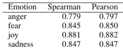
Since each tuple in this dataset was annotated by three annotators (odd number), we calculate SHR by randomly placing one or two annotations per tuple in one bin and the remaining (two or one) annotations for the tuple in another bin. Then two sets of intensity scores (and rankings) are calcu-lated from the annotations in each of the two bins. The process is repeated 100 times and the correla-tions across the two sets of rankings and intensity scores are averaged. Table2shows the split-half reliabilities for the anger, fear, joy, and sadness tweets in the Tweet Emotion Intensity Dataset.14 Observe that for fear, joy, and sadness datasets, both the Pearson correlations and the Spearman rank correlations lie between 0.84 and 0.88, indi-cating a high degree of reproducibility. However, 14Past work has found the SHR for sentiment intensity
an-notations for words, with 8 anan-notations per tuple, to be 0.98 (Kiritchenko et al.,2014). In contrast, here SHR is calculated from 3 annotations, for emotions, and from whole sentences. SHR determined from a smaller number of annotations and on more complex annotation tasks are expected to be lower.
Emotion Spearman Pearson anger 0.779 0.797 fear 0.845 0.850 joy 0.881 0.882 sadness 0.847 0.847
Table 2: Split-half reliabilities (as measured by Pearson correlation and Spearman rank correla-tion) for the anger, fear, joy, and sadness tweets in the Tweet Emotion Intensity Dataset.
the correlations are slightly lower for anger indi-cating that it is relative more difficult to ascertain the degrees of anger of speakers from their tweets. Note that SHR indicates the quality of annotations obtained when using only half the number of an-notations. The correlations obtained when repeat-ing the experiment with three annotations for each 4-tuple is expected to be even higher. Thus the numbers shown in Table 2are a lower bound on the quality of annotations obtained with three an-notations per 4-tuple.
5 Impact of Emotion Word Hashtags on Emotion Intensity
Some studies have shown that emoticons tend to be redundant in terms of the sentiment (Go et al., 2009; Mohammad et al., 2013). That is, if we remove a smiley face, ‘:)’, from a tweet, we find that the rest of the tweet still conveys a positive sentiment. Similarly, it has been shown that hashtag emotion words are also somewhat redundant in terms of the class of emotion being conveyed by the rest of the tweet (Mohammad,
2012). For example, removal of ‘#angry’ from the tweet below leaves a tweet that still conveys anger.
This mindless support of a demagogue needs to stop. #racism #grrr #angry
However, it is unclear what impact such emotion word hashtags have on the intensity of emotion. In fact, there exists no prior work to systematically study this. One of the goals of creating this dataset and including HQT–NQT tweet pairs, is to allow for exactly such an investigation.15
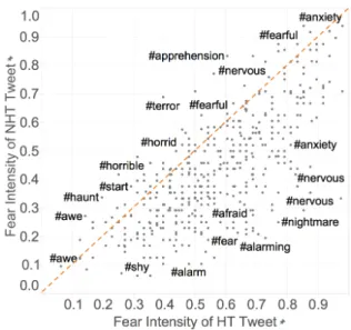
We analyzed the scores in our dataset to cre-ate scatter plots where each point corresponds to a HQT–NQT tweet pair, the x-axis is the emotion intensity score of the HQT tweet, and the y-axis is the score of the NQT tweet. Figure 1 shows the scatter plot for the fear data. We observe that
15
See Appendix (A.2) for further discussion on how emo-tion word hashtags have been used in prior research.
No. of HQT–NQT % Tweets Pairs Average Emotion Intensity Score Emotion Tweet Pairs Drop Rise None HQT tweets NQT tweets Drop Rise
anger 282 76.6 19.9 3.4 0.58 0.48 0.15 0.07
fear 454 86.1 13.9 4.4 0.57 0.43 0.18 0.07
joy 204 71.6 26.5 1.9 0.59 0.50 0.15 0.09
sadness 90 85.6 11,1 3.3 0.65 0.49 0.19 0.05
All 1030 78.6 17.8 3.6 0.58 0.47 0.17 0.08
Table 3: The impact of removal of emotion word hashtags on the emotion intensities of tweets.
Figure 1: The scatter plot of fear intensity of HQT tweet vs. corresponding NQT tweet. As per space availability, some points are labeled with the rele-vant hashtag.
in a majority of the cases, the points are on the lower-right side of the diagonal, indicating that the removal of the emotion word hashtag causes the emotion intensity of the tweet to drop. However, we do see a number of points on the upper-left side of the diagonal (indicating a rise), and some ex-actly on the diagonal (indicating no impact), due to the removal of a hashtag. Also observe that the removal of a hashtag can result in a drop in emo-tion scores for some tweets, but a rise for others (e.g., see the three labeled points for #nervous in the plot). We observe a similar pattern for other emotions as well (plots not shown here). Table3
summarizes these results by showing the percent-age of times the three outcomes occur for each of the emotions.
The table also shows that the average scores of HQT tweets and NQT tweets. The difference be-tween 0.58 and 0.47 is statistically significant.16 The last two columns show that when there is a drop in score on removal of the hashtag, the
aver-16
Wilcoxon signed-rank test at 0.05 significance level.
age drop is about 0.17 (17% of the total range 0– 1), whereas when there is a rise, the average rise is 0.08 (8% of the total range). These results show that emotion word hashtags are often not redun-dant with the rest of tweet in terms of what they bring to bear at the overall emotion intensity. Fur-ther, even though it is common for many of these hashtags to increase the emotion intensity, there is a more complex interplay between the text of the tweet and the hashtag which determines the di-rectionality and magnitude of the impact on emo-tion intensity. For instance, we often found that if the rest of the tweet clearly indicated the pres-ence of an emotion (through another emotion word hashtag, emojis, or through the non-hashtagged words), then the emotion word hashtag had only a small impact on the score.17
However, if the rest of the tweet is under-specified in terms of the emotion of the speaker, then the emotion word hashtag markedly in-creased the perceived emotion intensity. We also observed patterns unique to particular emotions. For example, when judging degree of fear of a speaker, lower scores were assigned when the speaker used a hashtag that indicated some outward judgment.
@RocksNRopes Can’t believe how rude your cashier was. fear: 0.48 @RocksNRopes Can’t believe how rude your cashier was. #terrible fear: 0.31 We believe that not vocalizing an outward judg-ment of the situation made the speaker appear more fearful. The HQT–NQT subset of our dataset will also be made separately, and freely, available as it may be of interest on its own, especially for the psychology and social sciences communities.
17
Unless the hashtag word itself is associated with very low emotion intensity (e.g., #peeved with anger), in which case, there was a drop in perceived emotion intensity.
Twitter Annotation Scope Label
AFINN (Nielsen,2011) Yes Manual Sentiment Numeric
BingLiu (Hu and Liu,2004) No Manual Sentiment Nominal
MPQA (Wilson et al.,2005) No Manual Sentiment Nominal
NRC Affect Intensity Lexicon (NRC-Aff-Int) (Mohammad,2017) Yes Manual Emotions Numeric
NRC Word-Emotion Assn. Lexicon (NRC-EmoLex) (Mohammad and Turney,2013) No Manual Emotions Nominal
NRC10 Expanded (NRC10E) (Bravo-Marquez et al.,2016) Yes Automatic Emotions Numeric
NRC Hashtag Emotion Association Lexicon (NRC-Hash-Emo) Yes Automatic Emotions Numeric
(Mohammad and Kiritchenko,2015)
NRC Hashtag Sentiment Lexicon (NRC-Hash-Sent) (Mohammad et al.,2013) Yes Automatic Sentiment Numeric
Sentiment140 (Mohammad et al.,2013) Yes Automatic Sentiment Numeric
SentiWordNet (Esuli and Sebastiani,2006) No Automatic Sentiment Numeric
SentiStrength (Thelwall et al.,2012) Yes Manual Sentiment Numeric
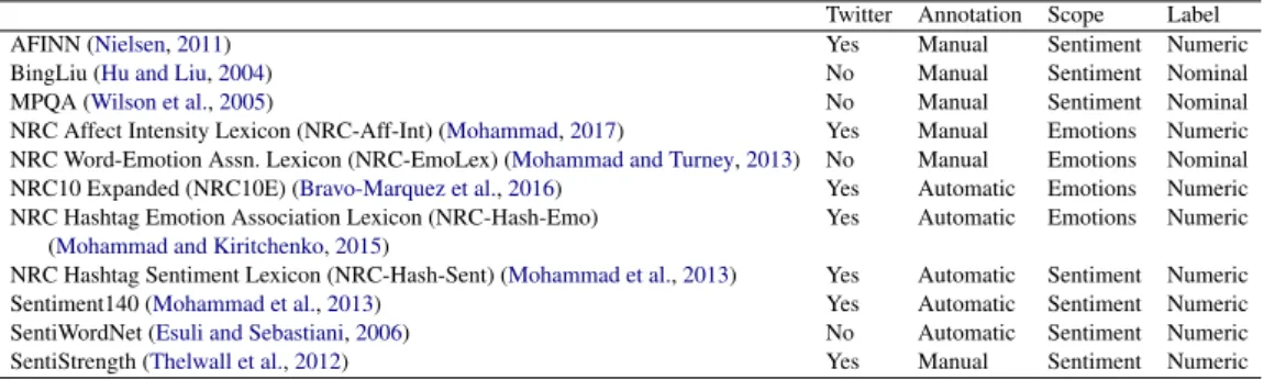
Table 4: Affect lexicons used in our experiments.
6 Automatically Determining Tweet Emotion Intensity
We now describe our regression system, which we use for obtaining benchmark prediction results on the new Tweet Emotion Intensity Dataset (Section
6.1) and for determining the extent to which two emotions are correlated (Section6.2).
Regression System We implemented a pack-age called AffectiveTweets for the Weka machine learning workbench (Hall et al., 2009) that pro-vides a collection of filters for extracting state-of-the-art features from tweets for sentiment classifi-cation and other related tasks. These include fea-tures used in Kiritchenko et al. (2014) and Mo-hammad et al. (2017).18 We use the package for calculating feature vectors from our emotion-intensity-labeled tweets and train Weka regression models on this transformed data. We used an L2 -regularized L2-loss SVM regression model with the regularization parameter C set to 1, imple-mented in LIBLINEAR19. The features used:20 a. Word N-grams (WN): presence or absence of word n-grams from n = 1 to n = 4.
b. Character N-grams (CN): presence or absence of character n-grams from n = 3 to n = 5. c. Word Embeddings (WE): an average of the word embeddings of all the words in a tweet. We calculate individual word embeddings using the negative sampling skip-gram model implemented in Word2Vec (Mikolov et al.,2013). Word vectors are trained from ten million English tweets taken from the Edinburgh Twitter Corpus (Petrovi´c et al., 2010). We set Word2Vec parameters:
18
Kiritchenko et al. (2014) describes the NRC-Canada system which ranked first in three sentiment shared tasks: 2013 Task 2, 2014 Task 9, and SemEval-2014 Task 4. Mohammad et al.(2017) describes a stance-detection system that outperformed submissions from all 19 teams that participated in SemEval-2016 Task 6.
19
http://www.csie.ntu.edu.tw/∼cjlin/liblinear/
20
See Appendix (A.3) for further implementation details.
window size: 5; number of dimensions: 400.21 d. Affect Lexicons (L): we use the lexicons shown in Table 4, by aggregating the information for all the words in a tweet. If the lexicon provides nominal association labels (e.g, positive, anger, etc.), then the number of words in the tweet matching each class are counted. If the lexicon provides numerical scores, the individual scores for each class are summed. These resources differ according to: whether the lexicon includes Twitter-specific terms, whether the words were manually or automatically annotated, whether the words were annotated for sentiment or emotions, and whether the affective associations provided are nominal or numeric. (See Table4.)
Evaluation We calculate the Pearson correla-tion coefficient (r) between the scores produced by the automatic system on the test sets and the gold intensity scores to determine the extent to which the output of the system matches the re-sults of human annotation.22 Pearson coefficient, which measures linear correlations between two variables, produces scores from -1 (perfectly in-versely correlated) to 1 (perfectly correlated). A score of 0 indicates no correlation.
6.1 Supervised Regression and Ablation We developed our system by training on the offi-cial training sets and applying the learned models to the development sets. Once system parameters were frozen, the system trained on the combined training and development corpora. These models were applied to the official test sets. Table5shows the results obtained on the test sets using various features, individually and in combination. The last column ‘avg.’ shows the macro-average of the cor-relations for all of the emotions.
21
Optimized for the task of word–emotion classification on an independent dataset (Bravo-Marquez et al.,2016).
22
We also determined Spearman rank correlations but these were inline with the results obtained using Pearson.
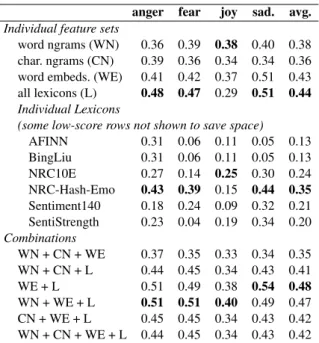
anger fear joy sad. avg.
Individual feature sets
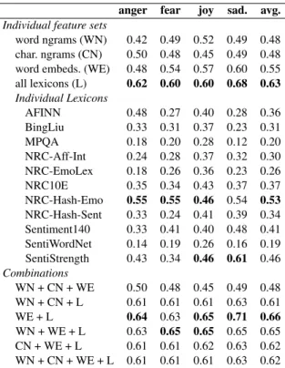
word ngrams (WN) 0.42 0.49 0.52 0.49 0.48 char. ngrams (CN) 0.50 0.48 0.45 0.49 0.48 word embeds. (WE) 0.48 0.54 0.57 0.60 0.55 all lexicons (L) 0.62 0.60 0.60 0.68 0.63 Individual Lexicons AFINN 0.48 0.27 0.40 0.28 0.36 BingLiu 0.33 0.31 0.37 0.23 0.31 MPQA 0.18 0.20 0.28 0.12 0.20 NRC-Aff-Int 0.24 0.28 0.37 0.32 0.30 NRC-EmoLex 0.18 0.26 0.36 0.23 0.26 NRC10E 0.35 0.34 0.43 0.37 0.37 NRC-Hash-Emo 0.55 0.55 0.46 0.54 0.53 NRC-Hash-Sent 0.33 0.24 0.41 0.39 0.34 Sentiment140 0.33 0.41 0.40 0.48 0.41 SentiWordNet 0.14 0.19 0.26 0.16 0.19 SentiStrength 0.43 0.34 0.46 0.61 0.46 Combinations WN + CN + WE 0.50 0.48 0.45 0.49 0.48 WN + CN + L 0.61 0.61 0.61 0.63 0.61 WE + L 0.64 0.63 0.65 0.71 0.66 WN + WE + L 0.63 0.65 0.65 0.65 0.65 CN + WE + L 0.61 0.61 0.62 0.63 0.62 WN + CN + WE + L 0.61 0.61 0.61 0.63 0.62 Table 5: Pearson correlations (r) of emotion inten-sity predictions with gold scores. Best results for each column are shown in bold: highest score by a feature set, highest score using a single lexicon, and highest score using feature set combinations.
Using just character or just word n-grams leads to results around 0.48, suggesting that they are reasonably good indicators of emotion intensity by themselves. (Guessing the intensity scores at random between 0 and 1 is expected to get correlations close to 0.) Word embeddings pro-duce statistically significant improvement over the ngrams (avg. r = 0.55).23 Using features drawn from affect lexicons produces results ranging from avg. r = 0.19 with SentiWordNet to avg. r = 0.53 with NRC-Hash-Emo. Combining all the lexicons leads to statistically significant improvement over individual lexicons (avg. r = 0.63). Combining the different kinds of features leads to even higher scores, with the best overall result obtained us-ing word embeddus-ing and lexicon features (avg. r = 0.66).24 The feature space formed by all the lexicons together is the strongest single feature category. The results also show that some fea-tures such as character ngrams are redundant in the presence of certain other features.
23
We used the Wilcoxon signed-rank test at 0.05 signifi-cance level calculated from ten random partitions of the data, for all the significance tests reported in this paper.
24
The increase from 0.63 to 0.66 is statistically significant.
Among the lexicons, NRC-Hash-Emo is the most predictive single lexicon. Lexicons that clude Twitter-specific entries, lexicons that in-clude intensity scores, and lexicons that label emotions and not just sentiment, tend to be more predictive on this task–dataset combination. NRC-Aff-Int has real-valued fine-grained word– emotion association scores for all the words in NRC-EmoLex that were marked as being associ-ated with anger, fear, joy, and sadness.25 Improve-ment in scores obtained using NRC-Aff-Int over the scores obtained using NRC-EmoLex also show that using fine intensity scores of word-emotion association are beneficial for tweet-level emotion intensity detection. The correlations for anger, fear, and joy are similar (around 0.65), but the cor-relation for sadness is markedly higher (0.71). We can observe from Table5that this boost in perfor-mance for sadness is to some extent due to word embeddings, but is more so due to lexicon fea-tures, especially those from SentiStrength. Sen-tiStrength focuses solely on positive and negative classes, but provides numeric scores for each. 6.1.1 Moderate-to-High Intensity Prediction In some applications, it may be more important for a system to correctly determine emotion inten-sities in the higher range of the scale than in the lower range of the scale. To assess performance in the moderate-to-high range of the intensity scale, we calculated correlation scores over a subset of the test data formed by taking only those instances with gold emotion intensity scores ≥ 0.5.
Table 6shows the results. Firstly, the correla-tion scores are in general lower here in the 0.5 to 1 range of intensity scores than in the experi-ments over the full intensity range. This is sim-ply because this is a harder task as now the sys-tems do not benefit by making coarse distinctions over whether a tweet is in the lower range or in the higher range. Nonetheless, we observe that many of the broad patterns of results stay the same, with some differences. Lexicons still play a crucial role, however, now embeddings and word ngrams are not far behind. SentiStrength seems to be less useful in this range, suggesting that its main bene-fit was separating low- and high-intensity sadness words. NRC-Hash-Emo is still the source of the most predictive lexicon features.
25
anger fear joy sad. avg.
Individual feature sets
word ngrams (WN) 0.36 0.39 0.38 0.40 0.38 char. ngrams (CN) 0.39 0.36 0.34 0.34 0.36 word embeds. (WE) 0.41 0.42 0.37 0.51 0.43 all lexicons (L) 0.48 0.47 0.29 0.51 0.44
Individual Lexicons
(some low-score rows not shown to save space)
AFINN 0.31 0.06 0.11 0.05 0.13 BingLiu 0.31 0.06 0.11 0.05 0.13 NRC10E 0.27 0.14 0.25 0.30 0.24 NRC-Hash-Emo 0.43 0.39 0.15 0.44 0.35 Sentiment140 0.18 0.24 0.09 0.32 0.21 SentiStrength 0.23 0.04 0.19 0.34 0.20 Combinations WN + CN + WE 0.37 0.35 0.33 0.34 0.35 WN + CN + L 0.44 0.45 0.34 0.43 0.41 WE + L 0.51 0.49 0.38 0.54 0.48 WN + WE + L 0.51 0.51 0.40 0.49 0.47 CN + WE + L 0.45 0.45 0.34 0.43 0.42 WN + CN + WE + L 0.44 0.45 0.34 0.43 0.42
Table 6: Pearson correlations on a subset of the test set where gold scores ≥ 0.5.
6.2 Similarity of Emotion Pairs
Humans are capable of hundreds of emotions, and some are closer to each other than others. One rea-son why certain emotion pairs may be perceived as being close is that their manifestation in language is similar, for example, similar words and expres-sion are used when expressing both emotions. We quantify this similarity of linguistic manifestation by using the Tweet Emotion Intensity dataset for the following experiment: we train our regression system (with features WN + WE + L) on the train-ing data for one emotion and evaluate predictions on the test data for a different emotion.
Table 7shows the results. The numbers in the diagonal are results obtained using training and test data pertaining to the same emotion. These results are upperbound benchmarks for the non-diagonal results, which are expected to be lower. We observe that negative emotions are positively correlated with each other and negatively corre-lated with the only positive emotion (joy). The absolute values of these correlations go from r = 0.23to r = 0.65. This shows that all of the emo-tion pairs are correlated at least to some extent, but that in some cases, for example, when learning from fear data and predicting sadness scores, one can obtain results (r = 0.63) close to the upper-bound benchmark (r = 0.65).26 Note also that the correlations are asymmetric. This means that even though one emotion may be strongly predictive of
26
0.63 and 0.65 are not statistically significantly different.
Test On
Train On anger fear joy sadness anger 0.63 0.37 -0.37 0.45 fear 0.46 0.65 -0.39 0.63 joy -0.41 -0.23 0.65 -0.41 sadness 0.39 0.47 -0.32 0.65
Table 7: Emotion intensity transfer Pearson corre-lation on all target tweets.
another, the predictive power need not be similar in the other direction. We also found that train-ing on a simple combination of both the fear and sadness data and using the model to predict sad-ness obtained a correlation of 0.67 (exceeding the score obtained with just the sadness training set).27 Domain adaptation may provide further gains.
To summarize, the experiments in this section show the extent to which two emotion are simi-lar as per their manifestation in language. For the four emotions studied here, the similarities vary from small (joy with fear) to considerable (fear with sadness). Also, the similarities are asymmet-ric. We also show that in some cases it is bene-ficial to use the training data for another emotion to supplement the training data for the emotion of interest. A promising avenue of future work is to test theories of emotion composition: e.g, whether optimism is indeed a combination of joy and an-ticipation, whether awe if fear and surprise, and so on, as some have suggested (Plutchik,1980).
7 Conclusions
We created the first emotion intensity dataset for tweets. We used best–worst scaling to improve annotation consistency and obtained fine-grained scores. We showed that emotion-word hashtags often impact emotion intensity, often conveying a more intense emotion. We created a benchmark regression system and conducted experiments to show that affect lexicons, especially those with fine word–emotion association scores, are use-ful in determining emotion intensity. Finally, we showed the extent to which emotion pairs are cor-related, and that the correlations are asymmetric— e.g., fear is strongly indicative of sadness, but sad-ness is only moderately indicative of fear.
Acknowledgment
We thank Svetlana Kiritchenko and Tara Small for helpful discussions.
27
0.67–0.63 difference is statistically significantly differ-ent, but 0.67–0.65 and 0.65–0.63 differences are not.
References
Cecilia Ovesdotter Alm, Dan Roth, and Richard Sproat. 2005. Emotions from text: Machine learn-ing for text-based emotion prediction. In Proceed-ings of the Joint Conference on HLT–EMNLP. Van-couver, Canada.
Saima Aman and Stan Szpakowicz. 2007. Identifying expressions of emotion in text. In Text, Speech and Dialogue, volume 4629 of Lecture Notes in Com-puter Science, pages 196–205.
Johan Bollen, Huina Mao, and Alberto Pepe. 2009. Modeling public mood and emotion: Twitter senti-ment and socio-economic phenomena. In Proceed-ings of the Fifth International Conference on We-blogs and Social Media. pages 450–453.
Felipe Bravo-Marquez, Eibe Frank, Saif M Moham-mad, and Bernhard Pfahringer. 2016. Determining word–emotion associations from tweets by multi-label classification. In Proceedings of the 2016 IEEE/WIC/ACM International Conference on Web Intelligence. Omaha, NE, USA, pages 536–539. Michael Brooks, Katie Kuksenok, Megan K
Torkild-son, Daniel Perry, John J RobinTorkild-son, Taylor J Scott, Ona Anicello, Ariana Zukowski, and Harris. 2013. Statistical affect detection in collaborative chat. In Proceedings of the 2013 conference on Computer supported cooperative work. San Antonio, Texas, USA, pages 317–328.
LJ Cronbach. 1946. A case study of the splithalf relia-bility coefficient. Journal of educational psychology 37(8):473.
Herbert Aron David. 1963. The method of paired com-parisons. Hafner Publishing Company, New York. Paul Ekman. 1992. An argument for basic emotions.
Cognition and Emotion6(3):169–200.
Andrea Esuli and Fabrizio Sebastiani. 2006. SENTI-WORDNET: A publicly available lexical resource for opinion mining. In Proceedings of the 5th Conference on Language Resources and Evaluation (LREC). Genoa, Italy, pages 417–422.
T. N. Flynn and A. A. J. Marley. 2014. Best-worst scal-ing: theory and methods. In Stephane Hess and An-drew Daly, editors, Handbook of Choice Modelling, Edward Elgar Publishing, pages 178–201.
Nico H Frijda. 1988. The laws of emotion. American psychologist43(5):349.
Kevin Gimpel, Nathan Schneider, et al. 2011. Part-of-speech tagging for Twitter: Annotation, features, and experiments. In Proceedings of the Annual Meeting of the Association for Computational Lin-guistics (ACL). Portland, OR, USA.
Alec Go, Richa Bhayani, and Lei Huang. 2009. Twit-ter sentiment classification using distant supervision. CS224N Project Report, Stanford1(12).
Mark Hall, Eibe Frank, Geoffrey Holmes, Bernhard Pfahringer, Peter Reutemann, and Ian H. Witten. 2009. The WEKA data mining software: An update. SIGKDD Explor. Newsl. 11(1):10–18.
https://doi.org/10.1145/1656274.1656278.
Minqing Hu and Bing Liu. 2004. Mining and summa-rizing customer reviews. In Proceedings of the tenth ACM SIGKDD international conference on Knowl-edge discovery and data mining. ACM, New York, NY, USA, pages 168–177.
David Jurgens. 2013. Embracing ambiguity: A com-parison of annotation methodologies for crowd-sourcing word sense labels. In Proceedings of the Annual Conference of the North American Chap-ter of the Association for Computational Linguistics. Atlanta, GA, USA.
David Jurgens, Saif M. Mohammad, Peter Turney, and Keith Holyoak. 2012. Semeval-2012 task 2: Mea-suring degrees of relational similarity. In Proceed-ings of the 6th International Workshop on Semantic Evaluation. Montr´eal, Canada, pages 356–364. Svetlana Kiritchenko and Saif M. Mohammad. 2016.
Capturing reliable fine-grained sentiment associa-tions by crowdsourcing and best–worst scaling. In Proceedings of The 15th Annual Conference of the North American Chapter of the Association for Computational Linguistics: Human Language Tech-nologies (NAACL). San Diego, California.
Svetlana Kiritchenko and Saif M. Mohammad. 2017. Best-worst scaling more reliable than rating scales: A case study on sentiment intensity annotation. In Proceedings of The Annual Meeting of the Associa-tion for ComputaAssocia-tional Linguistics (ACL). Vancou-ver, Canada.
Svetlana Kiritchenko, Xiaodan Zhu, and Saif M. Mo-hammad. 2014. Sentiment analysis of short infor-mal texts. Journal of Artificial Intelligence Research 50:723–762.
G Frederic Kuder and Marion W Richardson. 1937. The theory of the estimation of test reliability. Psy-chometrika2(3):151–160.
FA Kunneman, CC Liebrecht, and APJ van den Bosch. 2014. The (un) predictability of emotional hashtags in twitter. In Proceedings of the 5th Workshop on Language Analysis for Social Media. Gothenburg, Sweden, pages 26–34.
Jordan J. Louviere. 1991. Best-worst scaling: A model for the largest difference judgments. Working Paper. Jordan J. Louviere, Terry N. Flynn, and A. A. J. Mar-ley. 2015. Best-Worst Scaling: Theory, Methods and Applications. Cambridge University Press.
Tomas Mikolov, Kai Chen, Greg Corrado, and Jeffrey Dean. 2013. Efficient estimation of word represen-tations in vector space. In Proceedings of Workshop at ICLR.
Saif M. Mohammad. 2012. #Emotional tweets. In Pro-ceedings of the First Joint Conference on Lexical and Computational Semantics. Montr´eal, Canada, SemEval ’12, pages 246–255.
Saif M Mohammad. 2017. Word affect intensities. arXiv preprint arXiv:1704.08798.
Saif M. Mohammad and Felipe Bravo-Marquez. 2017. WASSA-2017 shared task on emotion intensity. In Proceedings of the Workshop on Computational Ap-proaches to Subjectivity, Sentiment and Social Me-dia Analysis (WASSA). Copenhagen, Denmark. Saif M. Mohammad and Svetlana Kiritchenko. 2015.
Using hashtags to capture fine emotion cate-gories from tweets. Computational Intelligence 31(2):301–326.https://doi.org/10.1111/coin.12024. Saif M. Mohammad, Svetlana Kiritchenko, and Xiao-dan Zhu. 2013. NRC-Canada: Building the state-of-the-art in sentiment analysis of tweets. In Pro-ceedings of the International Workshop on Semantic Evaluation. Atlanta, GA, USA.
Saif M. Mohammad, Parinaz Sobhani, and Svetlana Kiritchenko. 2017. Stance and sentiment in tweets. Special Section of the ACM Transactions on Inter-net Technology on Argumentation in Social Media 17(3).
Saif M. Mohammad and Peter D. Turney. 2013. Crowdsourcing a word–emotion association lexicon. Computational Intelligence29(3):436–465. Saif M. Mohammad, Xiaodan Zhu, Svetlana
Kir-itchenko, and Joel Martin. July 2015. Sentiment, emotion, purpose, and style in electoral tweets. In-formation Processing and Management 51(4):480– 499.
Alena Neviarouskaya, Helmut Prendinger, and Mit-suru Ishizuka. 2009. Compositionality principle in recognition of fine-grained emotions from text. In Proceedings of the Proceedings of the Third Inter-national Conference on Weblogs and Social Media (ICWSM-09). San Jose, California, pages 278–281. Finn ˚Arup Nielsen. 2011. A new ANEW: Evaluation
of a word list for sentiment analysis in microblogs. In Proceedings of the ESWC Workshop on ’Mak-ing Sense of Microposts’: Big th’Mak-ings come in small packages. Heraklion, Crete, pages 93–98.
Bryan Orme. 2009. Maxdiff analysis: Simple count-ing, individual-level logit, and HB. Sawtooth Soft-ware, Inc.
Alexander Pak and Patrick Paroubek. 2010. Twitter as a corpus for sentiment analysis and opinion mining. In Proceedings of the Conference on Language Re-sources and Evaluation (LREC). Malta.
W Parrot. 2001. Emotions in Social Psychology. Psy-chology Press.
Saˇsa Petrovi´c, Miles Osborne, and Victor Lavrenko. 2010. The Edinburgh Twitter corpus. In Proceed-ings of the NAACL HLT 2010 Workshop on Com-putational Linguistics in a World of Social Media. Association for Computational Linguistics, Strouds-burg, PA, USA, pages 25–26.
Robert Plutchik. 1980. A general psychoevolutionary theory of emotion. Emotion: Theory, research, and experience1(3):3–33.
Ashequl Qadir and Ellen Riloff. 2013. Bootstrapped learning of emotion hashtags# hashtags4you. In Proceedings of the 4th workshop on computational approaches to subjectivity, sentiment and social me-dia analysis. Atlanta, GA, USA, pages 2–11. Ashequl Qadir and Ellen Riloff. 2014. Learning
emo-tion indicators from tweets: Hashtags, hashtag pat-terns, and phrases. In Proceedings of the EMNLP Workshop on Arabic Natural Langauge Processing (EMNLP). Doha, Qatar, pages 1203–1209.
Kirk Roberts, Michael A Roach, Joseph Johnson, Josh Guthrie, and Sanda M Harabagiu. 2012. Em-patweet: Annotating and detecting emotions on Twitter. In Proceedings of the Conference on Lan-guage Resources and Evaluation. pages 3806–3813. James A Russell. 2003. Core affect and the psycholog-ical construction of emotion. Psychologpsycholog-ical review 110(1):145.
Carlo Strapparava and Rada Mihalcea. 2007. Semeval-2007 task 14: Affective text. In Proceedings of SemEval-2007. Prague, Czech Republic, pages 70– 74.
Anja Summa, Bernd Resch, Geoinformatics-Z GIS, and Michael Strube. 2016. Microblog emotion clas-sification by computing similarity in text, time, and space. In Proceedings of the PEOPLES Workshop at COLING. Osaka, Japan, pages 153–162.
Jared Suttles and Nancy Ide. 2013. Distant supervision for emotion classification with discrete binary val-ues. In Computational Linguistics and Intelligent Text Processing, Springer, pages 121–136.
Mike Thelwall, Kevan Buckley, and Georgios Pal-toglou. 2012. Sentiment strength detection for the social web. Journal of the American Society for In-formation Science and Technology63(1):163–173. Louis L. Thurstone. 1927. A law of comparative
judg-ment. Psychological review 34(4):273.
Theresa Wilson, Janyce Wiebe, and Paul Hoffmann. 2005. Recognizing contextual polarity in phrase-level sentiment analysis. In Proceedings of the Joint Conference on HLT and EMNLP. Stroudsburg, PA, USA, pages 347–354.
Frank Yates. 1936. Incomplete randomized blocks. Annals of Human Genetics7(2):121–140.
A Appendix
A.1 Best–Worst Scaling Questionnaire used to Obtain Emotion Intensity Scores The BWS questionnaire used for obtaining fear annotations is shown below.
Degree Of Fear In English Language Tweets The scale of fear can range from not fearful at all (zero amount of fear) to extremely fearful. One can often infer the degree of fear felt or expressed by a person from what they say. The goal of this task is to determine this degree of fear. Since it is hard to give a numerical score indicating the de-gree of fear, we will give you four different tweets and ask you to indicate to us:
• Which of the four speakers is likely to be the MOST fearful, and
• Which of the four speakers is likely to be the LEAST fearful.
Important Notes
• This task is about fear levels of the speaker (and not about the fear of someone else mentioned or spoken to).
• If the answer could be either one of two or more speakers (i.e., they are likely to be equally fearful), then select any one of them as the answer.
• Most importantly, try not to over-think the answer. Let your instinct guide you.
EXAMPLE
Speaker 1: Don’t post my picture on FB #grrr Speaker 2: If the teachers are this incompetent, I am afraid what the results will be.
Speaker 3: Results of medical test today #terrified Speaker 4: Having to speak in front of so many people is making me nervous.
Q1. Which of the four speakers is likely to be the MOST fearful?
– Multiple choice options: Speaker 1, 2, 3, 4 – Ans: Speaker 3
Q2. Which of the four speakers is likely to be the LEAST fearful?
– Multiple choice options: Speaker 1, 2, 3, 4 – Ans: Speaker 1
The questionnaires for other emotions are similar in structure. In a post-annotation survey, the re-spondents gave the task high scores for clarity of instruction (4.2/5) despite noting that the task it-self requires some non-trivial amount of thought (3.5 out of 5 on ease of task).
A.2 Use of Emotion Word Hashtags
Emotion word hashtags (e.g., #angry, #fear) have been used to search and compile sets of tweets that are likely to convey the emotions of interest. Often, these tweets are used in one of two ways: 1. As noisy training data for distant supervision (Pak and Paroubek,2010;Mohammad,2012; Sut-tles and Ide,2013). 2. As data that is manually annotated for emotions to create training and test datasets suitable for machine learning (Roberts et al., 2012;Qadir and Riloff,2014;Mohammad et al.,July 2015).28 We use emotion word hashtag to create annotated data similar to ‘2’, however, we use them to create separate emotion intensity datasets for each emotion. We also examine the impact of emotion word hashtags on emotion in-tensity. This has not been studied before, even though there is work on learning hashtags asso-ciated with particular emotions (Qadir and Riloff,
2013), and on showing that some emotion word hashtags are strongly indicative of the presence of an emotion in the rest of the tweet, whereas others are not (Kunneman et al.,2014).
A.3 AffectiveTweets Weka Package
AffectiveTweets includes five filters for converting tweets into feature vectors that can be fed into the large collection of machine learning algorithms implemented within Weka. The package is installed using the WekaPackageManager and can be used from the Weka GUI or the command line interface. It uses the TweetNLP library (Gimpel et al., 2011) for tokenization and POS tagging. The filters are described as follows.
• TweetToSparseFeatureVector filter: calculates the following sparse features: word n-grams (adding a NEG prefix to words occurring in negated contexts), character n-grams (CN), POS tags, and Brown word clusters.29
28
Often, the query term is removed from the tweet so as to erase obvious cues for a classification task.
29The scope of negation was determined by a simple
heuristic: from the occurrence of a negator word up until a punctuation mark or end of sentence. We used a list of 28 negator words such as no, not, won’t and never.
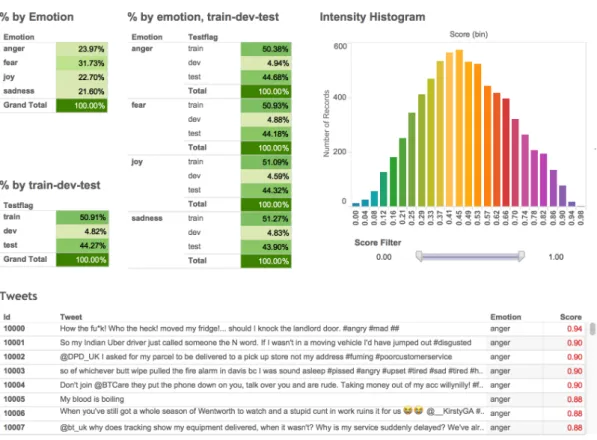
Figure 2: Screenshot of the interactive visualization to explore the Tweet Emotion Intensity Dataset. Available at: http://saifmohammad.com/WebPages/EmotionIntensity-SharedTask.html
• TweetToLexiconFeatureVector filter: calculates features from a fixed list of affective lexicons. • TweetToInputLexiconFeatureVector: calculates
features from any lexicon. The input lexicon can have multiple numeric or nominal word– affect associations.
• TweetToSentiStrengthFeatureVector filter: calculates positive and negative sentiment intensities for a tweet using the SentiStrength lexicon-based method (Thelwall et al.,2012) • TweetToEmbeddingsFeatureVectorfilter:
calcu-lates a tweet-level feature representation us-ing pre-trained word embeddus-ings supportus-ing the following aggregation schemes: average of word embeddings; addition of word embed-dings; and concatenation of the first k word em-beddings in the tweet. The package also pro-vides Word2Vec’s pre-trained word embeddings. Additional filters for creating affective lexicons from tweets and support for distant supervision are currently under development.
A.4 An Interactive Visualization to Explore the Tweet Emotion Intensity Dataset We created an interactive visualization to allow ease of exploration of this new dataset. The visualization has several components:
1. Tables showing the percentage of instances in each of the emotion partitions (train, dev, test). Hovering over a row shows the corresponding number of instances. Clicking on an emotion filters out data from all other emotions, in all visualization components. Similarly, one can click on just the train, dev, or test partitions to view information just for that data. Clicking again deselects the item.
2. A histogram of emotion intensity scores. A slider that one can use to view only those tweets within a certain score range.
3. The list of tweets, emotion label, and emotion intensity scores.
One can use filters in combination. For e.g., click-ing on fear, test data, and settclick-ing the slider for the 0.5 to 1 range, shows information for only those fear–testdata instances with scores ≥ 0.5.