Amplitude sampling for signal representation

(1)

Amplitude Sampling for Signal Representation

by

Pablo Martínez Nuevo

Ingeniero de Telecomunicación, University of Valladolid (2010)

M.S., Electrical Engineering, Columbia University (2012)

Submitted to the Department of Electrical Engineering and Computer

Science

in partial fulfillment of the requirements for the degree of

Doctor of Philosophy in Electrical Engineering and Computer Science

at the

MASSACHUSETTS INSTITUTE OF TECHNOLOGY

September 2016

c

○ Massachusetts Institute of Technology 2016. All rights reserved.

Author . . . .

Department of Electrical Engineering and Computer Science

August 30, 2016

Certified by . . . .

Alan V. Oppenheim

Ford Professor of Engineering

Thesis Supervisor

Accepted by . . . .

Professor Leslie A. Kolodziejski

Chairman, Department Committee on Graduate Theses

(2)

(3)

Amplitude Sampling for Signal Representation

by

Pablo Martínez Nuevo

Submitted to the Department of Electrical Engineering and Computer Science on August 30, 2016, in partial fulfillment of the

requirements for the degree of

Doctor of Philosophy in Electrical Engineering and Computer Science

Abstract

The theoretical basis for conventional acquisition of bandlimited signals typically re-lies on uniform time sampling and assumes infinite-precision amplitude values. This thesis explores signal representation and recovery based on uniform amplitude sam-pling with either assuming infinite-precision timing information or time restricted to a uniform grid. If time is allowed to lie on the continuum, the approach is based on a structure that is equivalent to reversibly transforming the input signal into a mono-tonic function which is then uniformly sampled in amplitude. In effect, the source signal is then implicitly represented by the times at which the monotonic function crosses a predefined set of amplitude values. We refer to this technique as amplitude sampling. This approach can be viewed alternatively as nonuniform time sampling of the original source signal whereas the resulting monotonic signal produces an associ-ated amplitude-time function which is uniformly sampled in amplitude. The duality and frequency-domain properties for the functions involved in the transformation are derived. Reconstruction from amplitude samples is shown to be possible through iterative algorithms. If both time and amplitude are restricted to equally-spaced val-ues, then the sampling strategy, referred to as lattice sampling, simultaneously uses both uniform amplitude and uniform time sampling. A class of bandlimited signals is characterized that can be sampled and reconstructed in this manner in order to derive spectral characteristics of quantized discrete-time signals.

Thesis Supervisor: Alan V. Oppenheim Title: Ford Professor of Engineering

(4)

(5)

Acknowledgments

This thesis is the result, to a greater or lesser extent, of contributions, at a technical or personal level, from many different people. A single individual cannot achieve on his own as much as they could with the collaboration, interaction, or support of the people around them. Naturally, chance is always present in the background. Therefore, the probability of my acknowledging everyone who has had an impact on this piece of work is arbitrarily close to zero. In fact, such is my gratitude to those that do appear in this section that my words below still sound like an understatement. I would like first to thank my research advisor Prof. Alan V. Oppenheim for giving me the opportunity of being under his mentorship. It is invaluable to have an advisor with such a true concern for the learning process of his students. Al, it has been a privilege to work with you in an environment of freedom and unconventional thinking.

I would also like to thank Prof. George C. Verghese and Dr. Petros T. Boufounos, both part of my thesis committee, for helping me shape the story of this thesis. To Hsin-Yu (Jane) Lai for going through the amplitude sampling process with me. To Guolong Su, my office mate, for many mathematically deep discussions. To DSPG for intellectually inspiring weekly meetings; this includes: Tom Baran, Petros Boufounos, Sefa Demirtas, Dan Dudgeon, Tarek Lahlou, Hsin-Yu (Jane) Lai, Catherine Medlock, Milutin Pajovic, and Guolong Su.

I would like to thank Prof. Yannis Tsividis at Columbia University for awakening my interest in research, and for believing in me when I knocked on his door.

I would like to express my deepest gratitude to my family. Thank you because I know I do not have to say thank you. In any case, I truly thank my parents, María Ángeles and Francisco, for always making every effort beyond measure so that my sister and I could pursue our intellectual curiosity. You have provided us with the most valuable education we could ever hope for. Thanks to my sister, Belén, for always being there. My family includes my wife, Ana. Thank you for walking beside me, for your selfless joy. Thank you for trimming the sail alongside me in this journey.

(6)

I am looking forward to embarking on our next adventure that, following the advice of my grandmother Mamita, should be closer to home.

Thanks also go to my friends in EECS and EAPS Building 25. Thank you for all the fun moments we have had together which have made this adventure a wonderful experience.

(7)

(8)

(9)

(10)

(11)

List of Figures

2-1 Principle of amplitude sampling by transformation of the source signal 𝑓 into a monotonic function 𝜑(𝑓 (𝑡)). . . 24 2-2 Equivalent representation of the amplitude sampling process. . . 25 2-3 Illustration of the parametrized transformation 𝑀𝛼 and its inverse 𝑀𝛼−1. 26

2-4 Illustration of the sampling points for the functions involved in ampli-tude sampling setting for a source signal 𝑓 (𝑡). . . 28 2-5 Example of the transformation in amplitude sampling where 𝑓 (𝑡) =

sinc(𝑡), 𝛼 = 1.38, and ℎ = 𝑀𝛼𝑓 . . . 30

3-1 Amplitude sampling involving the source signal 𝑓 and ℎ = 𝑀𝛼𝑓 ; (a)

nonuniform time sampling of 𝑓 ; (b) uniform amplitude sampling of ℎ. 40 3-2 Approximations to the bandlimited function 𝑓 by piecewise Taylor

polynomials centered around the sampling points 𝑥𝑛according to (3.2).

On the left, ˜𝑃 is a piecewise constant polynomial; on the right, ˜𝑃 is a piecewise second-degree polynomial. . . 42 3-3 Transformation of the operator 𝒜 based on samples of the original

function and its first 𝑁 derivatives for performing the successive ap-proximations in (3.5). . . 45 3-4 Block diagram of the proposed algorithm based on bandlimited

inter-polation of the uniform samples of ℎ. . . 48 3-5 Block diagram representation of the iterative amplitude sampling

(16)

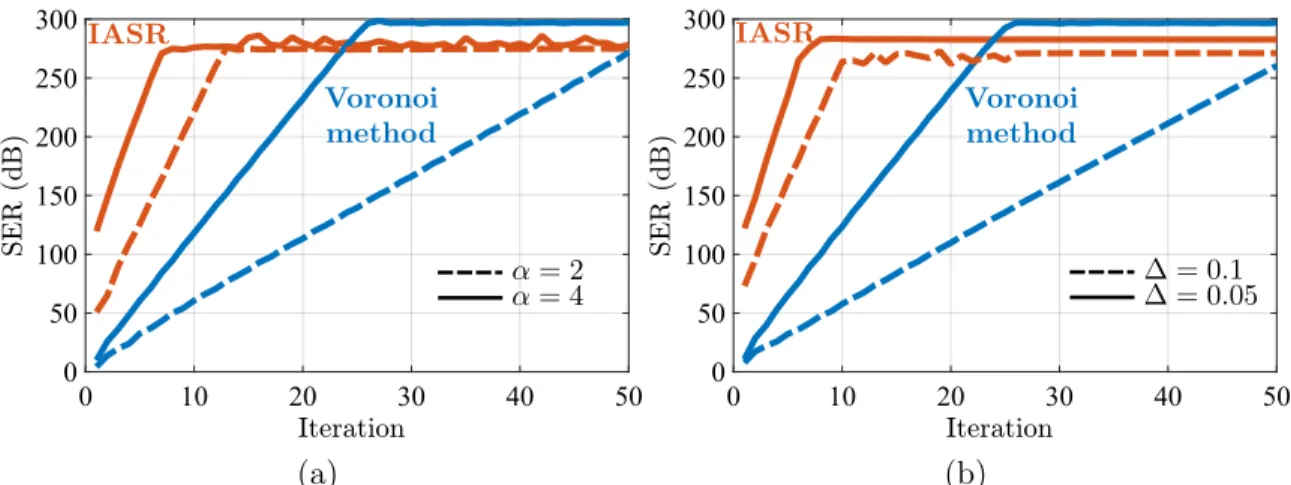
3-6 Performance comparison between IASR and the Voronoi method for a broadband input signal bandlimited and bounded; (a) 𝛼 is changed

while Δ is fixed; (b) Δ is changed while 𝛼 is fixed. . . 51

3-7 Performance comparison between IASR and the Voronoi method for broadband input signals bandlimited and bounded when their band-width 𝜎 is changed, and 𝛼 and Δ are fixed. . . 52

3-8 Performance comparison between IASR and the Voronoi method for a broadband input signal bandlimited and bounded when the sampling density is fixed and 𝛼 and Δ are changed. . . 53

4-1 (a) Illustration of the amplitude sampling mechanism; (b) schematic view of how to use a quantizer and a differentiator to produce the desired time sequence. . . 56

4-2 Encoder of a delta modulation system. . . 57

4-3 Asynchronous Delta Modulation Encoder. . . 58

4-4 Rectangular wave modulation encoder. . . 59

4-5 Explanation of the connection between amplitude sampling and rect-angular wave modulation. . . 61

4-6 Equivalence of the asynchronous sigma-delta modulation system and an integrator followed by a rectangular wave modulator. . . 63

5-1 Equivalent representation of an ADC consisting of a C/D block that performs uniform time sampling with period 𝑇 > 0 followed by a uni-form quantizer where Δ > 0 is the quantization step. . . 65

5-2 Example of lattice sampling. . . 66

5-3 Block-diagram illustration of the bandlimited interpolation, represented by a discrete-to-continuous (D/C) block, of a sequence generated by an ADC resulting in a lattice function. . . 67

(17)

5-4 Example of an integral-valued function pertaining to the set 𝒮, namely 𝑓 (𝑡) = 30 sin(𝜋𝑡)/𝜋(𝑡 + 1)(𝑡 − 2)(𝑡 + 3); (a) time-domain representation where the red dots represent the integer samples at integer points; (b) magnitude-squared of its Fourier transform. . . 73 5-5 Plot of the functions of Example 2 where 𝑓 (𝑡) ∈ 𝒮 and 𝑔(𝑡) ∈ ℬZ

𝜋. The

red dots represent crossings in the lattice points. . . 74 5-6 Bandwidth properties of a sequence generated by an ADC. The input

signal is assumed to have the appropriate decay conditions in order to produce a square-summable sequence. . . 80

6-1 Block-diagram representation of quantization as a homomorphism. . . 82 6-2 Quantizer block-diagram representation and its input-output

relation-ship for 𝐾 = 4 where 𝑥 ∈ R. For the sake of illustration, assume that 𝑄(𝑞𝑘) = 𝛿𝑘+1 for 𝑘 = 0, . . . , 3. . . 83

6-3 Bilevel quantizer. . . 84 6-4 In blue, input to a bilevel quantizer of the form depicted in Fig. 6-3;

in red, output of the quantizer. . . 84 6-5 As presented in Lemma 5, equivalency of operations when 𝜆 > 3𝜎 for

a signal 𝑓 bandlimited to 𝜎 rad/s . . . 91

7-1 Level-crossing samples; the horizontal dashed lines represent the am-plitude levels; the vertical dashed lines are placed at the time instants where the input signal crosses the corresponding amplitude level. . . . 94 7-2 Qualitative depiction of a function of the form (7.1) with three different

gaussian components. . . 96 7-3 Diagram on the complex plane for the derivation of the inequalities

used. The shaded region represents the possible locations of the pairs of complex conjugate zeros of the function considered denoted by {(𝑎𝑛, 𝑎*𝑛)′}𝑛∈Z

and the values (𝑅1,𝑘, 𝑅2,𝑘, 𝑡2,𝑘, 𝑡2,𝑘) specified in Theorem 10 for some

(18)

A-1 Illustration of the steps to prove Theorem 1. . . 113 A-2 The function 𝑔(𝑧) represents a holomorphic bijection between a disk of

radius 𝑅 and its image. The shaded regions represent the intersection of the respective images. The dashed circle represents the largest open disk with center 𝑔(𝑥′) such that it is completely contained in 𝑔(𝐷𝑅(𝑥′)).

The set 𝑆𝑎 is the region enclosed by the two dashed horizontal lines. . 116

C-1 Illustration of the relationship between the width of the region of ana-lyticity of a function 𝑓 and the decay at infinity of its Fourier transform, assuming 𝑓 meets the necessary decay and regularity conditions. The shaded area limited by dashed lines represents the region where the function is analytic. . . 134 C-2 Contours in color code used in the derivation of the classical sampling

theorem by means of Cauchy’s integral formula and the residue formula for some 0 < 𝜖𝑘 < 𝑘 + 1/2. . . 138

(19)

Chapter 1 Introduction

The interface between analog and digital signals is typically constituted by an analog-to-digital converter (ADC). The theoretical basis of this acquisition mechanism relies on the traditional sampling theorem [89, 37, 74], which describes the class of bandlim-ited signals by infinite-precision amplitude values taken at uniform instants of time. In this representation, the timing information is restricted to a uniform grid whereas the amplitude samples may assume values on a continuum.

In contrast, this thesis is about signal representation based on a discrete set of amplitude values considering either continuous or discrete time. This approach for signal representation has previously been studied and utilized in a number of context. The first attempts were focused on the zero crossings of the source signal. This idea was proposed in [8] within the more general theory of real and complex zeros of bandlimited signals. Logan’s theorem [50] describes a class of bandpass signals that can be completely described—within a scaling factor—by its zero crossings. Tractable recovery techniques only exist for periodic signals within the prescribed class [69]. Moreover, arbitrary bandlimited signals can be implicitly described by the zero crossings of a function resulting from an invertible transformation [27, 2, 39]—for example, the addition of a sinewave [21, Theorem 1]. In principle, interpolation is possible through Hadamard’s factorization [80, Chapter 5] although there are more efficient techniques in terms of convergence rate [73, 35, 76, 40]. Additionally, zero-crossings in the context of wavelet transforms have been considered in [51]. In this

(20)

case, stable reconstruction can be achieved by including additional information about the original signal.

The extension from zero crossings to multiple levels, in the context of data com-pression, was investigated in [52]. A sample is generated whenever the source signal crosses a predefined set of threshold levels. The time instants of the crossings and the level-crossings directions were utilized to represent the signal. Time was still quantized due to practical considerations. A practical continuous-time version of level-crossing sampling was later proposed in [84]. Asynchronous delta modulation [31] is, in some sense, a precursor of level-crossing sampling. It outputs a pulse, pos-itive or negative, at time instants when the change in signal amplitude surpasses a fixed quantity.

Our approach is to capitalize on uniform time sampling theory in the amplitude-time domain. In order to do so, we propose a sampling technique that is equivalent to reversibly transforming the source signal into a monotonic function which is then uniformly sampled in amplitude. We refer to this technique as amplitude sampling. The source signal is then implicitly represented by the times at which the signal crosses these amplitude levels. This procedure can alternatively be viewed as uniform sampling of an associated amplitude-time function.

In Chapter 2, we present the principle of amplitude sampling and derive duality as well time- and frequency-domain properties relating the functions involved in the transformation. The recovery from amplitude samples is carried out in Chapter 3. Amplitude sampling can be viewed as nonuniform time sampling of the source signal or as uniform amplitude sampling of the associated amplitude-time function. Recon-struction in both cases entails the use of iterative reconRecon-struction algorithms providing a necessary sampling density is satisfied. Chapter 4 shows the connection between amplitude sampling and delta-based modulation systems. For an appropriate choice of parameters, it can be shown that these systems perform nonuniform amplitude sampling of the associated amplitude-time function.

A generalization of either time or amplitude sampling is to restrict both amplitude and time values to a uniform grid. Then, a sample is taken at one of this

(21)

equally-spaced time instants only if the signal amplitude corresponds to one of the predefined threshold values. In other words, samples are generated when the signal crosses the points of a two-dimensional lattice. We refer to this approach as lattice sampling. Note that an ADC, with appropriately chosen parameters, transforms any input signal to a sequence whose bandlimited interpolation passes through these lattice points at every sampling instant.

Lattice sampling is developed in Chapter 5. We start by introducing the proper-ties of integral-valued polynomials elicited by the connection between polynomials and bandlimited functions discussed in Chapter 2. Then, we study the spectral character-istics of bandlimited functions that can be sampled and reconstructed in this manner and utilize these results in the analysis of the spectrum of quantized discrete-time signals.

The theoretical development in this thesis is mainly based on the complex-analytic perspective of bandlimited signals. In particular, we regard bandlimited signals as analytic functions on the whole complex plane with exponential growth, i.e. entire functions of exponential type. This framework establishes a connection between the analyticity of a function and the decay at infinity of its Fourier transform on the real line. Appendix C provides an overview of the main results within this framework. In addition, Appendix D includes some of the predominant approaches to nonuniform sampling reconstruction of bandlimited signals that we later refer to in Chapter 3.

The concept of quantization can be used to describe the proposed sampling tech-niques. Indeed, amplitude sampling quantizes the transformed signal with equal quantization steps and describes the input signal by the time instants at which it crosses these quantization levels. Then, lattice sampling incorporates quantization simultaneously both in time and amplitude. Alternatively, quantization can be con-sidered a part of the processing chain instead of that of the acquisition system. In this respect, we provide an example of the commutative property of one-level quan-tization as an operation on certain classes of signals. Chapter 6 formalizes this idea and presents the main concepts of quantization as a homomorphism.

(22)

usu-ally implementational simplicity. Thus, sampling is performed by quantizing the source signal, and recovery is achieved through a zero- or first-order hold, possi-bly in combination with low-pass filtering [53, 85]. Although there exist elaborate reconstruction techniques for multidimensional signals [93], advanced signal recon-struction techniques for generalized level-crossing sampling in one dimension are still under-explored. In the case of general bandlimited signals, it is still unclear how to guarantee a particular level-crossing sampling density. In Chapter 7, we provide suffi-cient conditions for a class of bandlimited signals in such a way that the level-crossing sampling density is guaranteed to satisfy Landau’s density criterion.

(23)

Chapter 2 Amplitude Sampling

2.1 Principle of Amplitude Sampling

Amplitude sampling, as proposed in this thesis, consists of reversibly transforming a source signal into a strictly monotonic function which is then uniformly sampled in amplitude. This process generates a sequence of analog time instants corresponding to the times at which successive levels are crossed. Since the transformed signal is strictly monotonic, there exists a one-to-one correspondence between amplitude values and time instants.

As illustrated in Fig. 2-1, the source signal 𝑓 is reversibly transformed into a strictly monotonic function 𝑢 = 𝜑(𝑓 (𝑡)) through a transformation 𝜑. Then, instead of time sampling 𝑢(𝑡), the function 𝑡(𝑢) is amplitude sampled on a uniform grid. This invertible transformation between time and amplitude is determined by the input signal. The time instants at which 𝜑(𝑓 (𝑡)) crosses the predefined set of amplitude values implicitly represent the source signal, i.e. 𝜑(𝑓 (𝑡𝑛)) = 𝑛Δ where Δ > 0 denotes

the separation between consecutive amplitude levels. Each of the time instants is paired with one amplitude level. Thus, the sequence of time instants contains enough information to describe the sampling process.

Since the transformation from time to amplitude is invertible, we will consider the analysis and realization of amplitude sampling in terms of the amplitude-time inverse function. Additionally, this sampling mechanism produces, to some extent, a

(24)

Figure 2-1: Principle of amplitude sampling by transformation of the source signal 𝑓 into a monotonic function 𝜑(𝑓 (𝑡)).

signal-dependent sampling density since the crossing times indirectly depend on the original signal. Despite this connection, the sampling density could, in principle, be controlled by the choice of the transformation 𝜑.

2.2 Transformation by Ramp Addition

While there are many ways of transforming the source signal into a monotonic func-tion, among the simplest is to add a ramp with sufficient slope. We assume the original signal 𝑓 is continuous, and it is possible to construct the strictly monotonic function 𝑢 = 𝑔(𝑡) = 𝛼𝑡 + 𝑓 (𝑡) for some 𝛼 ∈ R. Samples are then taken whenever 𝑔(𝑡) crosses the set of levels {𝑛Δ}, i.e.

𝑔(𝑡𝑛) = 𝑛Δ = 𝑓 (𝑡𝑛) + 𝛼𝑡𝑛 (2.1)

for all 𝑛 ∈ Z.

Equivalently, it is possible to obtain the same sequence of time instants {𝑡𝑛} by

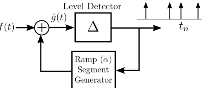
considering the block diagram in Fig. 2-2. The Level Detector outputs an impulse whenever its input takes the value Δ. In the feedback loop, the ramp-segment gen-erator takes as a reference the ramp 𝛼𝑡 that is shifted by an amount −Δ at times

(25)

Figure 2-2: Equivalent representation of the amplitude sampling process.

where the level detector generates an impulse. In other words,

˜

𝑔(𝑡) = 𝑓 (𝑡) + 𝛼𝑡 − 𝑘Δ (2.2)

for 𝑡 ∈ (𝑡𝑘, 𝑡𝑘+1] and 𝑘 ∈ Z. Thus,

˜

𝑔(𝑡𝑘+1) = Δ = 𝑓 (𝑡𝑘+1) + 𝛼𝑡𝑘+1− 𝑘Δ (2.3)

which gives (𝑘 + 1)Δ = 𝑔(𝑡𝑘+1) for all 𝑘 ∈ Z. Since there is a one-to-one

correspon-dence between amplitude values and time instants due to the monotonicity of 𝑔(𝑡), this implies that {𝑡𝑘} = {𝑡𝑛}. In summary, the procedure shown in Fig. 2-2, which

only involves bounded signals, generates impulses at the same time instants at which 𝑔(𝑡) crosses the set of amplitude levels {𝑛Δ}. The representation shown in Fig. 2-2 can be more convenient for practical purposes. However, for analysis purposes, we focus on the transformation of the source signal by ramp addition.

Since 𝑔(𝑡) is monotonic, there exists an inverse function 𝑔−1(𝑢) that we can choose to express in the form 𝑔−1(𝑢) = 𝑢/𝛼 + ℎ(𝑢) for some amplitude-time function ℎ. Al-though the transformation is from 𝑓 to 𝑔, the invertibility of the latter entails a bijective relationship between 𝑓 and ℎ. This interpretation suggests that this trans-formation can also be viewed as a mapping from 𝑓 to the associated function ℎ.

(26)

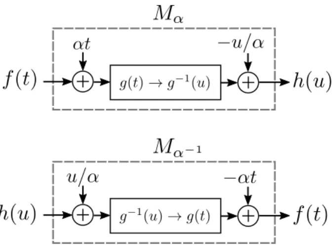
Figure 2-3: Illustration of the parametrized transformation 𝑀𝛼 and its inverse 𝑀𝛼−1.

2.2.1 Mapping between 𝑓 and ℎ

The addition of a ramp brings along a mapping, parametrized by the slope of the ramp, between the original signal and the function ℎ. First, we add the ramp 𝛼𝑡 to the input signal 𝑓 to construct the invertible function 𝑔. Then, inverting 𝑔 produces the function 𝑔−1 which after subtracting the ramp 𝑢/𝛼 generates ℎ. Let us denote this process by 𝑀𝛼, i.e. 𝑀𝛼𝑓 = ℎ. In the same way, we can reverse the procedure from ℎ

to 𝑓 by adding a ramp of slope 𝑢/𝛼 to ℎ and utilizing the invertibility of 𝑔−1 as well as the correspondence between 𝑔 and 𝑓 . Let us call this method 𝑀𝛼−1 that satisfies

𝑀𝛼−1. It is straightforward to see then that 𝑀_𝛼−1𝑀_𝛼−1 = 𝑀_𝛼−1𝑀_𝛼−1 = 𝐼 where 𝐼 is

the identity transformation. Note the this property is a consequence of the bijective relationship between 𝑔 and 𝑔−1. Fig. 2-3 illustrates the one-to-one correspondence between 𝑓 and ℎ.

The functions involved in the transformation are also connected by functional composition. In particular, the following equations are derived in [42]

𝑓 (𝑡) = − 𝛼ℎ(𝑓 (𝑡) + 𝛼𝑡) ℎ(𝑢) = − 1 𝛼𝑓 (ℎ(𝑢) + 𝑢 𝛼). (2.4)

It is possible to interpret (2.4) as a nonlinear time warping of the independent variable so as to obtain 𝑓 from ℎ or the reverse. The addition of a ramp in amplitude sampling

(27)

also generates an underlying mapping, dependent on 𝑓 or ℎ, between time 𝑡 and amplitude 𝑢. Both mappings can be easily captured in the following form

⎛ ⎝ 𝑓 (𝑡) 𝑡 ⎞ ⎠= ⎛ ⎝ −𝛼 0 1 1/𝛼 ⎞ ⎠ ⎛ ⎝ ℎ(𝑢) 𝑢 ⎞ ⎠ (2.5) ⎛ ⎝ ℎ(𝑢) 𝑢 ⎞ ⎠= ⎛ ⎝ −1/𝛼 0 1 𝛼 ⎞ ⎠ ⎛ ⎝ 𝑓 (𝑡) 𝑡 ⎞ ⎠ (2.6)

where both expressions are related through a matrix and its corresponding inverse. We have focused so far on the transformation from the point of view of 𝑓 , i.e. addition of a ramp with a sufficiently large slope and subsequent inversion of the resulting function. However, a duality in the transformation is evident in this repre-sentation. If we begin from knowledge of ℎ, the function 𝑓 is obtained by inverting ℎ and adding a ramp of appropriate slope. This is conceptually dual to starting with 𝑓 and constructing ℎ (see Fig. 2-3). In summary, this duality in the transformation es-tablishes a behavioral relationship between two functions, i.e. it does not distinguish between input and output. Moreover, it implies that any properties of ℎ inherited by assumptions made on 𝑓 hold, by duality, for 𝑓 if such assumptions are firstly imposed on ℎ.

2.2.2 The Sampling Process

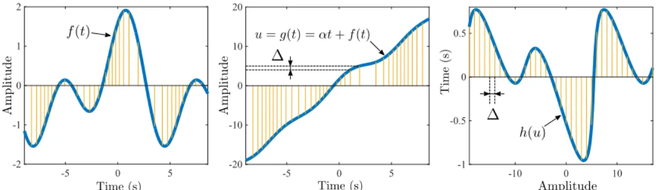
Amplitude sampling produces a sequence of time instants corresponding to 𝑛Δ = 𝑔(𝑡𝑛) = 𝛼𝑡𝑛 + 𝑓 (𝑡𝑛). Fig. 2-4 shows how, after the addition of a ramp of

suffi-ciently large slope, samples are taken whenever 𝑔 crosses an amplitude level. In the amplitude-time domain, this also corresponds to the inverse function 𝑔−1(𝑢) being uniformly sampled in amplitude, i.e. 𝑔−1(𝑛Δ) = 𝑛Δ/𝛼 + ℎ(𝑛Δ). Equivalently, ℎ is also sampled in a uniform grid, i.e.

(28)

-5 0 5 -20 -10 0 10 20 -5 0 5 -2 -1 0 1 2 -10 0 10 -1 -0.5 0 0.5

Figure 2-4: Illustration of the sampling points for the functions involved in amplitude sampling setting for a source signal 𝑓 (𝑡).

The timing information determines the sampling pairs for both 𝑓 and ℎ since 𝑓 (𝑡𝑛) = 𝑛Δ − 𝛼𝑡𝑛 for all 𝑛 ∈ Z. This naturally connects to time encoding techniques

since we can view amplitude sampling as producing the sequence {𝑡𝑛}. From that

sequence, we implicitly know the amplitude values providing the parameters involved are known. By duality, the recovery of ℎ uniquely determines 𝑓 and the reverse. For example, if ℎ is bandlimited and Δ is chosen accordingly, 𝑓 can be perfectly recovered.

2.2.3 Sampling Density

The times associated with the level crossings can in effect be interpreted as providing nonuniform time samples of the source signal. There are well known results on the required density of nonuniformly spaced samples in time of a bandlimited signal to permit perfect reconstruction. To explore the time sampling density implied by our amplitude sampling process, assume that the source signal 𝑓 is differentiable and with 𝐵 denoting the bound on the derivative, i.e. |𝑓′(𝑡)| ≤ 𝐵 for 𝐵 > 0. We can set the slope 𝛼 of the ramp such that |𝛼| > 𝐵, thus making 𝑔 a strictly monotonic function. Consider that 𝛼 is positive, the same conclusions follow analogously when 𝛼 < 0. Then, for large positive values of the derivative of 𝑓 , the slope of 𝑔 increases generating an increasing number of level crossings per unit of time. This situation is the opposite when 𝑓′ is close to −𝐵 since it reduces the slope of 𝑔. As a result, the signal 𝑓 (𝑡) is sampled more densely as its derivative becomes more positive and less densely as the derivative becomes more negative. Furthermore, reducing the value of

(29)

Δ leads to an increase in the overall level-crossing density.

Note that the derivative of 𝑔 is given by 𝑔′(𝑡) = 𝛼 + 𝑓′(𝑡) and is bounded by |𝛼| − 𝐵 ≤ |𝑔′(𝑡)| ≤ |𝛼| + 𝐵. (2.8) It is then clear that the time intervals between consecutive crossings can be bounded as:

Δ

|𝛼| + 𝐵 ≤ |𝑡𝑛+1− 𝑡𝑛| ≤ Δ

|𝛼| − 𝐵 (2.9)

for all 𝑛 ∈ Z. Equation (2.9) emphasizes the role that is played by the slope 𝛼 of the ramp and the quantizer step size Δ. It can be observed that if |𝛼| increases significantly, the bounds imply an almost uniform time spacing. Indeed, if the value of |𝛼| increases sufficiently, the contribution of 𝑓 in amplitude to the value of 𝑔 becomes less relevant. Thus, sampling 𝑔 would be close to the situation of sampling a straight line that, clearly, would generate a uniform time sequence.

2.3 Spectral Properties

In this section, we focus on properties of 𝑓 and consider the impact of these as-sumptions on the structure of ℎ = 𝑀𝛼𝑓 . In particular, we present results regarding

the spectral content of ℎ when the source signal 𝑓 is bandlimited. By duality, the corresponding conclusions apply to 𝑓 when ℎ is assumed to be bandlimited.

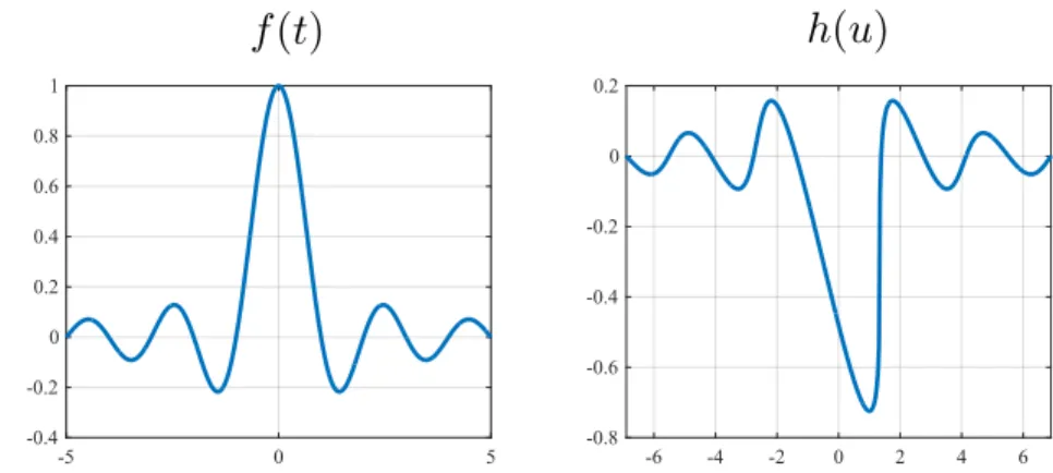
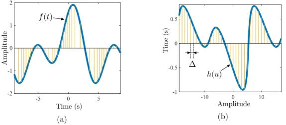
Consider the example in Fig. 2-5 with 𝑓 a sinc function—hence bandlimited—and 𝛼 is a positive number large enough to produce a monotonic function after the addition of the ramp. The shape of the function ℎ can be viewed as 𝑓 with a nonlinear warping of the independent variable. It presents shear-like parts that may manifest themselves as arbitrarily high-frequency content. These tilted regions in ℎ are due to the regions in 𝑓 with large negative values of the slope. Obviously, analogous conclusions can be drawn if 𝛼 is negative. Locally, the derivative of the inverse function is inversely proportional to that of the original function, then one may expect that the spectral content of ℎ is, in some sense, controlled by the difference |𝛼| − 𝐵, where |𝑓′(𝑡)| ≤ 𝐵

(30)

for all 𝑡 ∈ R. -5 0 5 -0.4 -0.2 0 0.2 0.4 0.6 0.8 1 -6 -4 -2 0 2 4 6 -0.8 -0.6 -0.4 -0.2 0 0.2

Figure 2-5: Example of the transformation in amplitude sampling where 𝑓 (𝑡) = sinc(𝑡), 𝛼 = 1.38, and ℎ = 𝑀𝛼𝑓 .

We formalize this notion in Theorem 1. In particular, it is assumed that 𝑓 is a bounded function and bandlimited to 𝜎 rad/s. In order to choose the slope of the ramp in the transformation 𝑀𝛼, we assumed above a bound for the first derivative

of the input function. In this case, we can utilize Bernstein’s inequality [5] that provides a bound on the real line for the derivative of a bounded bandlimited function. Specifically, if 𝑓 is bounded by some 𝐴 > 0, its derivative satisfies |𝑓′(𝑡)| ≤ 𝐴𝜎 for all 𝑡 ∈ R. Then, it is sufficient to choose |𝛼| > 𝐴𝜎 to construct the invertible transformation 𝑀𝛼. In doing so, we implicitly form the invertible function

𝑢 = 𝑔(𝑡) = 𝑓 (𝑡) + 𝛼𝑡 (2.10)

to derive ℎ(𝑢) = 𝑔−1(𝑢)−𝑢/𝛼. As a result, it can be shown that the Fourier transform of ℎ, denoted by ^ℎ(𝜉) for 𝜉 in Hz, satisfies |^ℎ(𝜉)| = 𝒪(𝑒−2𝜋|𝜉|𝑏), where 𝑏 > 0 is a function of the difference |𝛼| − 𝐴𝜎.

The precise statement is presented in the following theorem. Without loss of generality, the assumption about the decay on the real line of ℎ is included to produce clear proofs. However, it can be extended in a straightforward manner to square-integrable functions.

Theorem 1. Let 𝑓 (𝑡) : R → R be a continuous function bandlimited to 𝜎 > 0 rad/s. Assume further that |𝑓 (𝑡)| ≤ 𝐴/(1 + 𝑡2_{) for all 𝑡 ∈ R and some 𝐴 > 0. Construct the}

(31)

function

𝑢 = 𝑔(𝑡) = 𝛼𝑡 + 𝑓 (𝑡) (2.11) for |𝛼| > 𝐴𝜎. Then, there exists 𝑔−1_{(𝑢) for all 𝑢 ∈ R and a constant 𝐶 > 0 such} that the Fourier transform of ℎ(𝑢) = 𝑔−1(𝑢) − 𝑢/𝛼 satisfies |^ℎ(𝜉)| ≤ 𝐶𝑒−2𝜋|𝜉|𝑏 for any 0 ≤ 𝑏 < 𝑎 such that 𝑎 = |𝛼| 𝜎 log (︁|𝛼| 𝐴𝜎 )︁ − |𝛼| − 𝐴𝜎 𝜎 . (2.12) and 𝜉 ∈ R.

Proof. The detailed proof is carried out in Appendix A.

We expected the decay rate to be a function of |𝛼|−𝐴𝜎. In effect, the tilted regions in ℎ(𝑢), which are also the highest slope portions, correspond to more horizontal regions in 𝑔(𝑡). This is inherited from the properties of the inverse function. Indeed, note that 𝑔′_{(𝑡) ̸= 0 for all 𝑡 ∈ R, thus we can write (𝑔}−1(𝑢))′ = 1/𝑔′(𝑔−1(𝑢)). Loosely speaking, the slope of the inverse function 𝑔−1 is the reciprocal of the original function 𝑔. Therefore, if for example, 𝛼 > 0, regions with large negative values of 𝑓′ create regions in ℎ with large positive slopes. The latter are in turn responsible for the high-frequency content of ^ℎ. The influence of this effect is clearly controlled by the bound on the derivative of 𝑓 , or more precisely, by the difference |𝛼| − 𝐴𝜎.

In (2.12), we can clearly observe that the decay of the energy present in high frequencies depends on |𝛼| − 𝐴𝜎. The difference is logarithmic in the first term and linear in the second one. Since we have chosen |𝛼| > 𝐴𝜎, it always holds that 𝑎 > 0. This is consistent with our previous interpretation: the larger the difference the faster the decay at infinity.

It is important to note that the exponential decay of the spectrum of ℎ does not preclude ℎ from being bandlimited, i.e. any bandlimited signal has a Fourier transform that belongs to 𝒪(𝑒−2𝜋|𝜉|𝑏) as |𝜉| → ∞ for any 𝑏 ̸= 0. The next theorem states that, if the signal 𝑓 is bandlimited, the function ℎ cannot also be bandlimited unless 𝑓 is a constant.

(32)

Theorem 2. Under the conditions of Theorem 1 and unless 𝑓 is constant, the func-tion ℎ(𝑢) is nonbandlimited for every |𝛼| > 𝐴𝜎 with at most one excepfunc-tion.

Proof. The detailed proof is carried out in Appendix B.

This theorem clarifies that if 𝑓 is a nonconstant bandlimited function, then ℎ = 𝑀𝛼𝑓 is guaranteed to be nonbandlimited. Strictly speaking, there may exist a value

of 𝛼 for which we cannot make such assertion. This is due to the fact that in the proof a theorem is used (referred to as Picard’s little theorem) that states that an analytic function on the whole complex plane assumes every value in C with the possible exception of a single point. For practical purposes, we ignore this singular case.

In summary, if the function 𝑓 is assumed to be bandlimited and nonconstant, then ℎ = 𝑀𝛼𝑓 is nonbandlimited and with an exponential decay in its spectrum. In

some sense, the function ℎ becomes closer to a bandlimited function as |𝛼| increases. Recall from (2.4) that 𝑓 (𝑡) = −𝛼ℎ(𝑓 (𝑡) + 𝛼𝑡). This implies that 𝑓 is close to ℎ for sufficiently large |𝛼| and after appropriate scaling of the axes.

2.4 Decay Properties

We have seen that, in some sense, ℎ inherits some of the characteristics of 𝑓 since the former is a close deformed version of the latter. Therefore, it is useful to explore more specifically the connections between the properties of 𝑓 and ℎ in the time domain. In particular, it is reasonable to think that the properties on the real line may be similar between the two.

2.4.1 Moderate Decrease

Note that the inverse function of a straight line with slope 𝛼 ̸= 0 is another ramp with slope 1/𝛼. Our intuition suggests that if we subtract from 𝑔−1(𝑢) a straight line with slope 1/𝛼, this would result in a function with decay properties akin to 𝑓 . The initial choice of the expression of ℎ explicitly entails the subtraction of a ramp of

(33)

slope 1/𝛼 from 𝑔−1. However, it is possible to choose a different value for the slope. The following lemma formalizes this intuition by stating that for any other ramp with slope different from 1/𝛼, ℎ does not decay appropriately on the real line.

Proposition 1. Under the conditions of Theorem 1, construct the function ℎ(𝑢) = 𝑔−1_{(𝑢) − 𝛽𝑢 for some 𝛽 ∈ R. Then, the function ℎ(𝑢) is of moderate decrease if and} only if 𝛽 = 1/𝛼.

Proof. The backward direction, i.e. assuming 𝛽 = 1/𝛼, has been proved in Theorem 1. For the forward direction, assume on the contrary that 𝛽 ̸= 1/𝛼. From (A.14), we have the following bound

⃒ ⃒ ⃒|𝑔 −1 (𝑢)| − |𝑢|/𝛼 ⃒ ⃒ ⃒≤ 𝐴/𝛼. (2.13)

Therefore, using the reverse triangle inequality and the previous expression, we arrive at the following for large enough 𝑢

|ℎ(𝑢)| = |𝑔−1(𝑢) − 𝛽𝑢| ≥ ⃒ ⃒ ⃒|𝑔 −1 (𝑢)| − 𝛽|𝑢| ⃒ ⃒ ⃒≥ ⃒ ⃒ ⃒|𝑢| ⃒ ⃒ ⃒𝛽 − 1 𝛼 ⃒ ⃒ ⃒− 𝐴 𝛼 ⃒ ⃒ ⃒. (2.14) Clearly, the right-hand side grows linearly without bound. Thus, |ℎ(𝑢)| is unbounded for 𝛽 ̸= 1/𝛼 and cannot be of moderate decrease.

2.4.2 𝐿

𝑝

norms

In order to gain a deeper understanding of the transformation 𝑀𝛼, it is interesting to

see how it modifies the size, in terms of 𝐿𝑝 norms, of the respective functions. Thus, we show in the following results how the norms of 𝑓 and ℎ are related. As one may expect, the parameter 𝛼 plays a crucial role.

Proposition 2. Under the conditions of Theorem 1, the following relationship holds

(𝛼 − 𝐴𝜎)1/𝑝

𝛼 ||𝑓 ||𝑝 ≤ ||ℎ||𝑝 ≤

(𝛼 + 𝐴𝜎)1/𝑝

𝛼 ||𝑓 ||𝑝. (2.15) for 1 ≤ 𝑝 < ∞. Furthermore, this implies that ||𝑓 ||∞ = 𝛼||ℎ||∞.

(34)

Proof. The following equations hold [42] ℎ(𝑓 (𝑡) + 𝛼𝑡) = −1 𝛼 𝑓 (𝑡) 𝑓(︁ℎ(𝑢) + 1 𝛼𝑢 )︁ = −𝛼ℎ(𝑢). (2.16)

If we perform the change of variables 𝑢 = 𝑓 (𝑡) + 𝛼𝑡, we can derive for 1 ≤ 𝑝 < ∞

||ℎ||𝑝_𝑝 = ∫︁ R |ℎ(𝑢)|𝑝d𝑢 = ∫︁ R |ℎ(𝑓 (𝑡) + 𝛼𝑡)|𝑝(𝑓′(𝑡) + 𝛼)d𝑡 ≤ ∫︁ R |ℎ(𝑓 (𝑡) + 𝛼𝑡)|𝑝_{(𝛼 + 𝐴𝜎)d𝑡 =} (𝛼 + 𝐴𝜎) 𝛼𝑝 ∫︁ R |𝑓 (𝑡)|𝑝_d𝑡 = (𝛼 + 𝐴𝜎) 𝛼𝑝 ||𝑓 || 𝑝 𝑝

where we have also used the fact that sup_𝑡∈R|𝑓′_{(𝑡) + 𝛼| ≤ (𝛼 + 𝐴𝜎).}

In order to find the reverse inequality, we first have to find a bound for |ℎ′(𝑢)+1/𝛼| by noting that inf𝑡∈R|𝑓′(𝑡) + 𝛼| = 𝛼 − 𝐴𝜎, i.e.

|ℎ′(𝑢) + 1/𝛼| = |(𝑔−1(𝑢))′| =⃒⃒ ⃒ 1 𝑔′_(𝑔−1_(𝑢)) ⃒ ⃒ ⃒= ⃒ ⃒ ⃒ 1 𝑓′_(𝑔−1_{(𝑢)) + 𝛼} ⃒ ⃒ ⃒≤ 1 𝛼 − 𝐴𝜎. (2.17) Using again (2.16) and the change of variables 𝑡 = ℎ(𝑦) + 𝑦/𝛼, we obtain

||𝑓 ||𝑝_𝑝 = ∫︁ R |𝑓 (ℎ(𝑢) + 1 𝛼𝑢)| 𝑝 (ℎ′(𝑢) + 1 𝛼)d𝑢 ≤ 𝛼𝑝 𝛼 − 𝐴𝜎||ℎ|| 𝑝 𝑝

which proves the lower bound. If we now let 𝑝 → ∞ in (2.15), we get ||𝑓 ||∞ =

𝛼||ℎ||∞.

The main conclusion is that the decay properties on the real line of 𝑓 are inherited by ℎ in the sense that if 𝑓 ∈ 𝐿𝑝_{(R), then ℎ ∈ 𝐿}𝑝_{(R). The previous proposition shows}

precise bounds for the 𝐿𝑝 norms of ℎ with respect to 𝑓 and vice versa. It is interesting to note that the 𝐿∞ norm is controlled by 𝛼. Indeed, for very large values of 𝛼, the ramp approaches the vertical axis, thus reducing the range of ℎ.

We can go one step further and give a specific relationship between the 𝐿𝑝 _norms

(35)

𝑝 < ∞ since we have assumed it is bounded and of moderate decay. In particular, if 𝑓 ∈ 𝐿𝑝_{(R), then} ∫︀

R|𝑓 (𝑡)|

𝑝+1_{d𝑡 ≤ 𝐴}∫︀

R|𝑓 (𝑡)|

𝑝_{d𝑡, which implies that 𝑓 ∈ 𝐿}𝑝+1_(R).

Since 𝑓 is of moderate decay is absolutely integrable and, by induction, we see that the claim is true.

||ℎ||𝑝 =

1 𝛼1−1𝑝

||𝑓 ||𝑝 (2.18)

whenever 1 ≤ 𝑝 < ∞.

Proof. Using again (2.16) and the change of variables 𝑢 = 𝑓 (𝑡) + 𝛼𝑡, it is clear that for any even number 𝑝

||ℎ||𝑝 𝑝 = ∫︁ R ℎ(𝑓 (𝑡) + 𝛼𝑡)𝑝(𝑓′(𝑡) + 𝛼)d𝑡 = 1 𝛼𝑝 ∫︁ R 𝑓 (𝑡)𝑝𝑓′(𝑡)d𝑡 + 1 𝛼𝑝−1||𝑓 || 𝑝 𝑝. (2.19)

We now show that the first term on the right-hand side vanishes. First note that by the fundamental theorem of calculus we have that ∫︀

R𝑓

′_{(𝑡)d𝑡 = 0 for any continuous}

function satisfying lim|𝑡|→∞𝑓 (𝑡) = 0. Thus, we arrive at the following

∫︁ R 𝑓 (𝑡)𝑝𝑓′(𝑡)d𝑡 = 1 𝑝 + 1 ∫︁ R (𝑓 (𝑡)𝑝+1)′d𝑡 = 0 (2.20) since 𝑓 (𝑡)𝑝+1 _{is also of moderate decay. Therefore, ||ℎ||}

𝑝 = ||𝑓 ||𝑝/𝛼(𝑝−1)/𝑝.

Now, for any number 𝑝 ≥ 1 we can write ∫︁ R |𝑓 (𝑡)|𝑝_𝑓′ (𝑡)d𝑡 =∑︁ 𝑛∈Z ∫︁ 𝑎𝑛+1 𝑎𝑛 𝑓 (𝑡)𝑝𝑓′(𝑡)d𝑡 −∑︁ 𝑚∈Z ∫︁ 𝑏𝑚+1 𝑏𝑚 𝑓 (𝑡)𝑝𝑓′(𝑡)d𝑡 (2.21) where 𝑓 (𝑡) ≥ 0 for 𝑡 ∈ (𝑎𝑛, 𝑎𝑛+1) and 𝑓 (𝑡) ≤ 0 for 𝑡 ∈ (𝑏𝑚, 𝑏𝑚+1) for all 𝑚, 𝑛 ∈ Z.

Thus, for each 𝑛 ∈ Z we have ∫︁ 𝑎𝑛+1 𝑎𝑛 𝑓 (𝑡)𝑝𝑓′(𝑡)d𝑡 = 𝑓 (𝑡) 𝑝+1 𝑝 + 1 ⃒ ⃒ ⃒ 𝑎𝑛+1 𝑎𝑛 = 0 (2.22)

(36)

Note that we allow to have intervals of the form (𝑐, ∞) or (−∞, 𝑑) for any 𝑐, 𝑑 ∈ R and the same holds true since lim|𝑡|→∞𝑓 (𝑡)𝑝+1= 0 for 𝑝 ≥ 1. Therefore, we have that

∫︁

R

|𝑓 (𝑡)|𝑝_𝑓′

(𝑡)d𝑡 = 0 (2.23)

and ||ℎ||𝑝 = ||𝑓 ||𝑝/𝛼(𝑝−1)/𝑝 for any number 𝑝 ≥ 1.

This last result clearly presents an improvement over Proposition 2. The relation-ship between the norms does not depend on the difference 𝛼 − 𝐴𝜎 like the decay of the spectrum of ℎ. As long as 𝛼 > 𝐴𝜎, the size of the functions in terms of 𝐿𝑝 norms only depend on the magnitude of alpha.

Let 𝑓1 and 𝑓2 generate ℎ1 and ℎ2 respectively under the assumptions of Theorem

1. Could we expect that ℎ1 and ℎ2 are close if 𝑓1 and 𝑓2 are close? We prove in the

following proposition that if they are close in terms of the distance metric induced by the 𝐿1 _{norm, then ℎ}

1 and ℎ2 are close. Moreover, the distance is exactly the same.

||ℎ1− ℎ2||1 = ||𝑓1 − 𝑓2||1. (2.24)

Proof. Note that |ℎ1(𝑢)−ℎ2(𝑢)| = |𝑔1−1(𝑢)−𝑔 −1

2 (𝑢)| and |𝑓1(𝑡)−𝑓2(𝑡)| = |𝑔1(𝑡)−𝑔2(𝑡)|,

thus by Fubini’s theorem we arrive at the following

||ℎ1− ℎ2||1 = ∫︁ R |𝑔₁−1(𝑢) − 𝑔−1₂ (𝑢)|d𝑢 = ∫︁ R2 1Γd𝑡d𝑢 ||𝑓1− 𝑓2||1 = ∫︁ R |𝑔1(𝑡) − 𝑔2(𝑡)|d𝑡 = ∫︁ R2 1Λd𝑡d𝑢 where Γ = {(𝑡, 𝑢) ∈ R2 : 𝑡 ∈ R, min{𝑔1(𝑡), 𝑔2(𝑡)} ≤ 𝑢 ≤ max{𝑔1(𝑡), 𝑔2(𝑡)}} Λ = {(𝑡, 𝑢) ∈ R2 : 𝑢 ∈ R, min{𝑔−11 (𝑢), 𝑔 −1 2 (𝑢)} ≤ 𝑡 ≤ max{𝑔 −1 1 (𝑢), 𝑔 −1 2 (𝑢)}}.

For an arbitrary (𝑡𝑜, 𝑢𝑜) ∈ Γ, we have that 𝑡𝑜 ≤ max{𝑔−11 (𝑢𝑜), 𝑔2−1(𝑢𝑜)} and 𝑡𝑜 ≥

(37)

Using the same reasoning we obtain Γ ⊆ Λ which implies that Γ = Λ. Thus, the integrals are the same.

2.4.3 Slope Sensitivity

In the development of amplitude sampling, we have assumed that, starting from the source signal 𝑓 , the associated amplitude-time function ℎ is constructed by subtract-ing a ramp of slope 1/𝛼 from 𝑔−1(𝑢). Indeed, this is the reciprocal slope of the linear element in 𝑔(𝑡) = 𝛼𝑡 + 𝑓 (𝑡). Moreover, according to Proposition 1, it is the only choice that generates an ℎ with similar decay conditions as the source signal 𝑓 . In-stead, it is also possible to construct ℎ(𝑢) = 𝑔−1_{(𝑢) − 𝛽𝑢 where 𝛽 ∈ R. In this case,} the invertibility of the transformation from ℎ to 𝑓 is not affected even if 𝛽 ̸= 1/𝛼. However, the decay conditions of 𝑓 are not transferred to ℎ in the same manner for arbitrary values of 𝛽. The next proposition provides bounds that characterize the growth behavior of ℎ on the real line.

Proposition 5. Under the conditions of Proposition 1, the function ℎ(𝑢) = 𝑔−1(𝑢) − 𝛽𝑢 admits the following bounds

|𝑢(𝛽 − 1 𝛼)| − 𝐴 𝛼 ≤ |ℎ(𝑢)| ≤ |𝑢(𝛽 − 1 𝛼)| + 𝐴 𝛼 (2.25) for all 𝑢 ∈ R.

Proof. From Proposition 3, we have that |𝑔−1_{(𝑢) − 𝑢/𝛼| ≤ 𝐴/𝛼 for all 𝑢 ∈ R. Then,} it follows that |ℎ(𝑢)| = |𝑔−1(𝑢)−𝑢 𝛼−𝑢(𝛽 − 1 𝛼)| ≤ |𝑔 −1 (𝑢)−𝑢 𝛼|+|𝑢(𝛽 − 1 𝛼)| ≤ |𝑢(𝛽 − 1 𝛼)|+ 𝐴 𝛼 (2.26) where we have applied the triangle inequality. The lower bound follows analogously from the reverse triangle inequality.

This result can also be viewed as a generalized form of the 𝐿∞norm when the ramp subtracted from 𝑔−1(𝑢) is not exactly 1/𝛼. Indeed, if the ramp component in 𝑔−1 is

(38)

not completely removed, then Proposition 5 characterizes the residual linear element in ℎ. In other words, assuming ℎ is desired to decay at infinity, it characterizes the sensitivity of this procedure when the reciprocal slope is set inaccurately, i.e. 𝛽 ̸= 1/𝛼. As a result, ℎ grows linearly at a rate determined by the difference 𝛽 − 1/𝛼.

2.5 Summary

Amplitude sampling is based on reversibly transforming the source signal before per-forming uniform amplitude sampling. Thus, there exists a one-to-one correspondence between the input signal and an associated amplitude-time function. This perspec-tive allows the sampling process to be uniform in the amplitude domain. Among the myriad of possible transformations of the input signal, we chose the addition of a ramp. The invertibility of the transformation is not affected by choosing the slopes of both ramps different from the reciprocal of one another. However, the latter produces a residual linear element in the resulting function. A duality in this transformation manifests itself in the bidirectional relationship between assumptions and properties of the functions involved. In particular, we concluded that both functions cannot be simultaneously bandlimited unless they are both constant. Moreover, the bandlimit-edness of one forces a spectrum with exponential decay on the other. Regarding their decay characteristics, we showed how this behavior is the same except for the slope of the added ramp as a multiplicative factor. In fact, these properties are all dependent on the slope of the source signal and the added ramp.

(39)

Chapter 3 Reconstruction in Amplitude

Sampling

The amplitude sampling process is composed of several functions each characterized by a sampling structure. Consider the transformation of the source signal 𝑓 (𝑡) as the addition of a ramp of sufficiently large slope. Then, the function 𝑔(𝑡) = 𝛼𝑡 + 𝑓 (𝑡) is nonuniformly sampled in time since the sampling instants correspond to the times at which 𝑔 crosses a predefined set of amplitude levels. Clearly, this sampling sequence is dependent on the source signal. Equivalently, the samples of 𝑔 are in a one-to-one correspondence to those of 𝑓 , thus the source signal is also nonuniformly time sampled. Alternatively, due to the monotonicity of 𝑔, we can regard the sampling process in the amplitude-time domain through the inverse function 𝑔−1(𝑢). In fact, 𝑔−1(𝑢) is uniformly sampled in the amplitude domain. Likewise, the function ℎ(𝑢) = (𝑀𝛼𝑓 )(𝑢) = 𝑔−1(𝑢) − 𝑢/𝛼 is uniform sampled in amplitude. Fig. 3-1 depicts sampling

from both perspectives: time and amplitude.

Reconstruction can then be performed as a nonuniform sampling problem in the time domain or as a uniform sampling problem in the amplitude domain. In the first case, the initial assumption is that 𝑓 is bandlimited irrespective of the impact on ℎ, and we introduce nonuniform sampling reconstruction techniques in this setting. In the second case, we start with the assumption that ℎ is bandlimited without con-sidering its implications for 𝑓 . Then, we assume 𝑓 is bandlimited and, although ℎ

(40)

-5 0 5 -2 -1 0 1 2 (a) -10 0 10 -1 -0.5 0 0.5 (b)

Figure 3-1: Amplitude sampling involving the source signal 𝑓 and ℎ = 𝑀𝛼𝑓 ; (a)

nonuniform time sampling of 𝑓 ; (b) uniform amplitude sampling of ℎ.

cannot be bandlimited simultaneously, we describe an iterative reconstruction tech-nique based on bandlimited interpolation of the uniform samples of ℎ.

3.1 Iterative Reconstruction Algorithms from

Nonuni-form Samples

We have already seen that the frame operator could be used for signal reconstruction from nonuniform samples. If we have a sampling sequence {𝑥𝑛}𝑛∈Z that satisfies

Jaffard’s result, i.e. Theorem 21, then it can be shown that the frame operator, in that case, takes the form

𝒮𝑓 =∑︁

𝑛∈Z

𝑓 (𝑥𝑛)sinc((𝑥 − 𝑥𝑛)𝜎/𝜋). (3.1)

for 𝑓 ∈ 𝐵𝑀 where 𝑀 = 𝜎/𝜋. In principle, we can reconstruct the function 𝑓

ban-dlimited to 𝜎 rad/s by means of Proposition 20. However, the main downside of this operator is that we do not have explicit estimates for the frame bounds, which makes estimating the rate of convergence very difficult.

In order to circumvent this problem, it is possible to consider different types of operators. In [25], it is shown how to construct an operator by first approximating

(41)

with a piecewise constant function and then lowpass filtering. In fact, we generalize this result by considering samples of the function and its derivatives. In this situation, it is possible to improve significantly the rate of convergence of the algorithm.

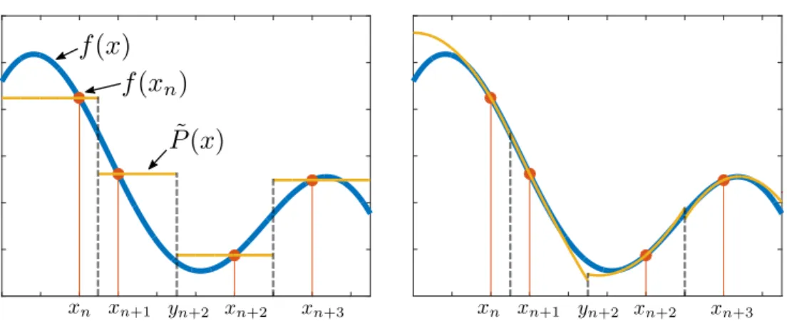
Fig. 3-2 show how the operator functions in its initial stage. On the left-hand side, a piecewise constant function is given by 𝑃𝑛(𝑥) = 𝑓 (𝑥𝑛) whenever 𝑥 ∈ [𝑦𝑛, 𝑦𝑛+1)

for 𝑦𝑛 = (𝑥𝑛+ 𝑥𝑛−1)/2 and 𝑛 ∈ Z. This is the approach followed in [25]. However,

if the samples of the first 𝑁 derivatives at {𝑥𝑛}𝑛∈Z can also be incorporated, we can

generalize this idea and use piecewise Taylor polynomials of degree 𝑁 in the same intervals. Specifically, write

𝑃𝑛(𝑥) = 1[𝑦𝑛,𝑦𝑛+1)(𝑥) 𝑁 ∑︁ 𝑘=0 𝑓(𝑘)_(𝑥 𝑛) 𝑘! (𝑥 − 𝑥𝑛) 𝑘 _(3.2)

This case corresponds to the right-hand plot in Fig. 3-2 where second-degree poly-nomials are considered. It is obvious that if 𝑁 = 0, then it reduces to the usual piecewise constant approximation.

The picture suggests that as the degree of the polynomial increases, the distance between 𝑓 and ˜𝑃 = ∑︀

𝑛∈Z𝑃𝑛(𝑥) may reduce in the 𝐿

2_{-norm sense providing that the}

maximum separation of sampling points is small enough. Thus, it appears that the result of lowpass filtering ˜𝑃 would be closer to 𝑓 as the degree increases.

In any case, for this approach to work, we need samples of the function and its first 𝑁 derivatives, which requires access to more information than in the initial scenario. Intuitively, it is reasonable that the performance of the reconstruction algorithm improves since we have more a priori information about the original signal. In some sense, it feels natural to consider samples of the derivatives of a bandlimited function. Note that these functions can be analytically extended to the whole complex plane. As a result, they are completely described by a power series—which consists of values of their derivatives—centered around any point in C.

Let us call 𝒫 the orthogonal projection from 𝐿2_{(R) to 𝐵}𝑀, i.e. lowpass filtering.

Assume that we obtain the pair {𝑥𝑛, 𝑓 (𝑥𝑛)}𝑛∈Z from a nonuniform sampling process.

(42)

approxima-0.2 -0.1 0 0.1 0.2 0.3 0.4 0.5 0.6 0.7

Figure 3-2: Approximations to the bandlimited function 𝑓 by piecewise Taylor poly-nomials centered around the sampling points 𝑥𝑛 according to (3.2). On the left,

˜

𝑃 is a piecewise constant polynomial; on the right, ˜𝑃 is a piecewise second-degree polynomial.

tion to the function 𝑓 . Fig. 3-2 shows the piecewise Taylor polynomial, which is then lowpass filtered. We show in the next theorem, that we can reconstruct 𝑓 iteratively using the operator 𝒜. However, the following two inequalities are necessary. The first one is Wirtinger’s inequality [29, p. 184].

Lemma 1. (Wirtinger’s Inequality) Let 𝑓, 𝑓′ ∈ 𝐿2_{([𝑎, 𝑏]) such that either 𝑓 (𝑎) = 0}

or 𝑓 (𝑏) = 0, then ∫︁ 𝑏 𝑎 |𝑓 (𝑥)|2d𝑥 ≤ 4 𝜋2(𝑏 − 𝑎) 2 ∫︁ 𝑏 𝑎 |𝑓′(𝑥)|2d𝑥. (3.3) We are also going to need a modified version of Bernstein’s inequality involving 𝐿2 norms. For more details, refer to [4, 94].

Lemma 2. (Bernstein’s inequality) If 𝑓 (𝑧) is an entire function of exponential type 𝜎, then for 𝑝 ≥ 1

||𝑓′||𝑝 ≤ 𝜎||𝑓 ||𝑝 (3.4)

By the Paley-Wiener theorem, we know that any continuous function 𝐵𝑀 is an

entire function of exponential type 𝜎 = 2𝜋𝑀 . Thus, from Bernstein’s inequality, we conclude that ||𝑓′||2 ≤ 𝜎||𝑓 ||2. Now, we are ready to prove the following result where

(43)

Theorem 3. Assume 𝛿 = sup_𝑛∈Z|𝑥𝑛+1 − 𝑥𝑛| < 𝜋/𝜎, 𝜎 = 2𝜋𝑀 for some 𝑀 >

0, and 𝑃𝑛(𝑥) is the 𝑁 -th degree Taylor polynomial described in (3.2). Then, 𝑓 ∈

𝐵𝑀 is uniquely determined by the samples {(𝑥𝑛, 𝑓 (𝑥𝑛), . . . , 𝑓(𝑁 )(𝑥𝑛))}𝑛∈Z and can be

reconstructed by the following iteration

𝑓0 = 𝒜𝑓 = 𝒫 (︁ ∑︁ 𝑛∈Z 𝑃𝑛(𝑥)1[𝑦𝑛,𝑦𝑛+1) )︁ 𝑓𝑘+1 = 𝑓𝑘+ 𝒜(𝑓 − 𝑓𝑘) (3.5)

for 𝑘 ≥ 0 and 𝑦𝑛 = (𝑥𝑛+ 𝑥𝑛−1)/2. Then, lim𝑘→∞𝑓𝑘 = 𝑓 in 𝐿2(R) and

||𝑓 − 𝑓𝑘||2 ≤

(︁𝛿𝜎 𝜋

)︁(𝑁 +1)(𝑘+1)

||𝑓 ||2. (3.6)

Furthermore, the following bounds hold

||𝒜𝑓 ||2 ≤ (︁ 1 +(︁𝛿𝜎 𝜋 )︁(𝑁 +1))︁ ||𝑓 ||2 ||𝒜−1𝑓 ||2 ≤ (︁ 1 +(︁𝛿𝜎 𝜋 )︁(𝑁 +1))︁−1 ||𝑓 ||2. (3.7)

Proof. It is clear that 𝑓 = 𝒫𝑓 = 𝒫(∑︀

𝑛∈Z𝑓 1[𝑦𝑛,𝑦𝑛+1)), thus we can write

||𝑓 − 𝒜𝑓 ||2 2 = ||𝒫( ∑︁ 𝑛∈Z 𝑓 − 𝑃𝑛(𝑥)1[𝑦𝑛,𝑦𝑛+1))|| 2 2 ≤ ||∑︁ 𝑛∈Z 𝑓 − 𝑃𝑛(𝑥)1[𝑦𝑛,𝑦𝑛+1)|| 2 2 = ∑︁ 𝑛∈Z ∫︁ 𝑦𝑛+1 𝑦𝑛 |𝑓 (𝑥) − 𝑃𝑛(𝑥)|2d𝑥. (3.8)

We can split the last integral in (3.8) in the following way ∫︁ 𝑥𝑛 𝑦𝑛 |𝑓 (𝑥) − 𝑃𝑛(𝑥)|2d𝑥 + ∫︁ 𝑦𝑛+1 𝑥𝑛 |𝑓 (𝑥) − 𝑃𝑛(𝑥)|2d𝑥. (3.9)

(44)

where we have used the fact that (𝑥𝑛− 𝑦𝑛) ≤ 𝛿/2 and (𝑦𝑛+1− 𝑥𝑛) ≤ 𝛿/2. Since we

constructed the polynomials 𝑃𝑛 to satisfy 𝑃 (𝑗)

𝑛 (𝑥𝑛) = 𝑓(𝑗)(𝑥𝑛) for 0 ≤ 𝑗 ≤ 𝑁 and

𝑛 ∈ Z, we can again split the last part of (3.10) as in (3.9) and apply Wirtinger’s inequality. In fact, we can repeat this procedure 𝑁 + 1 times obtaining

∫︁ 𝑥𝑛 𝑦𝑛 |𝑓 (𝑥) − 𝑃𝑛(𝑥)|2d𝑥 + ∫︁ 𝑦𝑛+1 𝑥𝑛 |𝑓 (𝑥) − 𝑃𝑛(𝑥)|2d𝑥 ≤(︁𝛿 𝜋 )︁2(𝑁 +1)∫︁ 𝑦𝑛+1 𝑦𝑛 |𝑓(𝑁 +1)_{(𝑥)|d𝑥.} (3.11)

Then, it is immediate to conclude

∑︁ 𝑛∈Z ∫︁ 𝑦𝑛+1 𝑦𝑛 |𝑓 (𝑥) − 𝑃𝑛(𝑥)|2d𝑥 ≤ (︁𝛿 𝜋 )︁2(𝑁 +1) ||𝑓(𝑁 +1)_||2 _≤(︁𝛿𝜎 𝜋 )︁2(𝑁 +1) ||𝑓 ||2 (3.12)

where we have used Lemma 2 in the last inequality. The latter implies that

||𝑓 − 𝒜𝑓 || ≤(︁𝛿𝜎 𝜋

)︁(𝑁 +1)

||𝑓 ||. (3.13)

Therefore, 𝒜 is bounded and invertible on ℬ𝜎 with the following bounds

||𝒜𝑓 || < ||𝑓 || + ||𝒜𝑓 − 𝑓 || ≤(︁1 +(︁𝛿𝜎 𝜋 )︁(𝑁 +1))︁ ||𝑓 || (3.14) and similarly ||𝒜−1𝑓 || = || ∞ ∑︁ 𝑘=0 (ℐ −𝒜)𝑘𝑓 || ≤ ∞ ∑︁ 𝑘=0 (︁𝛿𝜎 𝜋 )︁(𝑁 +1)𝑘 ||𝑓 || =(︁1+ (︁𝛿𝜎 𝜋 )︁(𝑁 +1))︁−1 ||𝑓 ||. (3.15)

(45)

Figure 3-3: Transformation of the operator 𝒜 based on samples of the original function and its first 𝑁 derivatives for performing the successive approximations in (3.5).

If we now apply Proposition 20, we obtain the desired properties for the iteration. We can visualize the acquisition process in Theorem 3 as depicted in Fig. 3-3. The first approximation denoted by 𝑓0 corresponds precisely to block diagram in this

figure. Subsequent refinements are performed based on this approximation for the difference (𝑓 − 𝑓𝑘). It is important to note the the rate of convergence is faster at

the expense of including more information about the signal, namely samples of the derivatives.

3.2 Amplitude Sampling:

Recovery from

Nonuni-form Samples

In the time domain, amplitude sampling generates nonuniform samples of the source signal 𝑓 (𝑡), i.e. 𝑓 (𝑡𝑛) = 𝑛Δ − 𝛼𝑡𝑛 for all 𝑛 ∈ Z. As shown in Appendix D, there are

several conditions that the sampling instants have to satisfy in order to have any hope for perfect reconstruction. In the following lemma, we state sufficient conditions such that perfect recovery from amplitude samples is possible through iterative techniques providing the original signal is bandlimited.

Lemma 3. Let 𝑓 (𝑡) ∈ 𝐵𝑀 be a function such that sup_𝑡∈R|𝑓 (𝑡)| ≤ 𝐴. Assume further

that {𝑡𝑛}𝑛∈Z satisfies 𝑓 (𝑡𝑛) = 𝑛Δ − 𝛼𝑡𝑛 for some Δ > 0 and 𝛼 > 𝐴2𝜋𝑀 > 0. If Δ <

(46)

Furthermore, 𝑓 can be reconstructed by means of the following iteration for 𝑘 ≥ 0

𝑓0 = 𝒮𝑓 (3.16)

𝑓𝑘+1 = 𝑓𝑘+ 𝒮(𝑓 − 𝑓𝑘) (3.17)

where 𝒮 is the frame operator given by

𝒮𝑓 = ∑︁

𝑛∈Z

𝑓 (𝑡𝑛)sinc(2𝑀 (𝑡 − 𝑡𝑛)) (3.18)

Proof. The derivative of 𝑔(𝑡) is given by 𝑔′(𝑡) = 𝛼 + 𝑓′(𝑡) and is bounded by

𝛼 − 𝐴𝜎 ≤ |𝑔′(𝑡)| ≤ 𝛼 + 𝐴𝜎 (3.19) where 𝜎 = 2𝜋𝑀 . This implies that

Δ

𝛼 + 𝐴𝜎 ≤ |𝑡𝑛+1− 𝑡𝑛| ≤ Δ

𝛼 − 𝐴𝜎. (3.20)

It is then clear that the sequence {𝑡𝑛}𝑛∈Z is relatively separated. Now, if we choose

Δ < (𝛼 + 𝐴𝜎)𝜋/𝜎, it is guaranteed that 𝐷−({𝑡𝑛}𝑛∈Z) > 𝜎/𝜋. By Jaffard’s theorem

[33], {sinc((𝑡 − 𝑡𝑛)𝜎/𝜋)}𝑛∈Z generates a frame for 𝐵𝑀. According to Proposition 20,

we can then use the frame operator 𝒮𝑓 =∑︀

𝑛∈Z𝑓 (𝑡𝑛)sinc((𝑡 − 𝑡𝑛)𝜎/𝜋) to iteratively

recover 𝑓 .

Clearly, it is straightforward to appropriately choose the parameters in amplitude sampling to guarantee the desired properties for the sampling sequence. Although there exists a myriad of nonuniform sampling reconstruction techniques [25], we made use of the frame operator in Lemma 3 with the purpose of showing the existence of iterative reconstruction techniques from amplitude samples.

(47)

3.3 Amplitude Sampling: Recovery from Uniform

Samples

We focus on reconstruction techniques that rely on the uniform samples of the func-tion ℎ. As a first approach, we suppose ℎ is bandlimited. Then, the bandlimitedness assumption is imposed on 𝑓 , and we describe how to iteratively recover 𝑓 by ban-dlimitied interpolation of the nonbandlimited function ℎ.

3.3.1 Nonuniform Sampling of Nonbandlimited Signals

Amplitude sampling can be viewed as uniformly sampling the function ℎ = 𝑀𝛼𝑓 for

a source signal 𝑓 and an appropriate choice of 𝛼. If we are able to reconstruct ℎ from uniform samples, then the input signal 𝑓 can of course also be recovered due to the invertibility of 𝑀𝛼.

Suppose the functions ℎ are bounded by some 𝐵 > 0 and bandlimited to 𝜎 rad/s. Assume now that we perform amplitude sampling on signals 𝑓 that can be written in the form 𝑓 = 𝑀1/𝛼ℎ for a fixed 1/𝛼 > 𝐵𝜎. Note that these signals are

nonbandlim-ited since the assumption of bandlimnonbandlim-itedness lies in the functions ℎ. In particular, they belong to a subset of nonbandlimited signals whose Fourier transform decays at least exponentially fast. Then, amplitude sampling generates the pair of samples {𝑡𝑛, 𝑓 (𝑡𝑛)}𝑛∈Z where 𝑛Δ = 𝛼𝑡𝑛+ 𝑓 (𝑡𝑛). Clearly, this mechanism generates a

nonuni-form sampling set for the function 𝑓 . Essentially, we are nonuninonuni-formly sampling a nonbandlimited signal.

Moreover, we are performing simultaneously uniform sampling on ℎ with a sample spacing of Δ. Obviously, if we choose Δ < 𝜋/𝜎 satisfying the Nyquist rate, we can then reconstruct ℎ from the classical sampling theorem. This implies that 𝑓 can be perfectly recovered through the interpolation of ℎ. In principle, any bandlimited function passed through an invertible nonlinearity is recoverable from its uniform samples if the nonlinearity is perfectly known. In our case, the invertible nonlinearity corresponds to 𝑀1/𝛼.

(48)

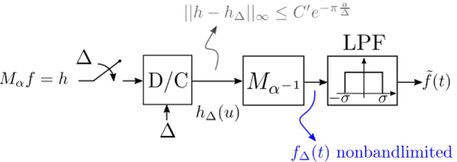
Figure 3-4: Block diagram of the proposed algorithm based on bandlimited interpo-lation of the uniform samples of ℎ.

3.3.2 Approximate Recovery

We assume now that 𝑓 is bandlimited and perform bandlimited interpolation from samples of ℎ. Fig. 3-4 shows a block diagram of the proposed scheme. The starting point corresponds to the set of uniform samples of the function ℎ, i.e. ℎ(𝑛Δ) = 𝑡𝑛− 𝑛Δ/𝛼 of all 𝑛 ∈ Z, which are related to the nonuniform samples of 𝑓 by a scaling

and a sign change 𝑓 (𝑡𝑛) = −𝛼𝑡𝑛+ 𝑛Δ. First, a bandlimited approximation, denoted

by D/C in the figure, is performed with parameter Δ > 0, i.e.

ℎΔ(𝑢) =

∑︁

𝑘∈Z

ℎ(𝑘Δ)sinc(𝑢/Δ − 𝑘). (3.21)

Since ℎ is nonbandlimited, then the output ℎΔ is an approximate version of ℎ due

to the aliasing error incurred. In fact, this aliasing error has been characterized in [88, 9] in terms of the 𝐿∞ norm. In our setting, this error can be bounded as shown in the following proposition.

Proposition 6. If ℎΔ is the bandlimited approximation to ℎ, then there exists a

𝐶′ > 0 such that ||ℎ − ℎΔ||∞≤ 𝐶′ 𝑎 𝑒 −𝜋𝑎 Δ (3.22) where 𝑎 = 𝛼_𝜎 log(_𝐴𝜎𝛼 ) − 𝛼−𝐴𝜎_𝜎 .

Proof. Since ℎ(𝑢) is continuous and of moderate decrease, ^ℎ(𝜉) is also continuous. Moreover, we know from Theorem 1 that |^ℎ(𝜉)| ≤ 𝐶𝑒−𝑎2𝜋|𝜉| for 𝑎 defined in (A.11) and some 𝐶 > 0. Clearly, ^ℎ is Lebesgue measurable and absolutely integrable. Thus,

(49)

by the generalized form of Weiss’s theorem [10] we can bound the approximation error as |ℎ(𝑢) − ℎΔ(𝑢)| ≤ 2 ∫︁ |𝜉|>1/2Δ |^ℎ(𝜉)|d𝜉 ≤ 4𝐶 ∫︁ 𝜉>1/2Δ 𝑒−2𝜋𝜉𝑎d𝜉 = 4𝐶 2𝜋𝑎𝑒 −𝜋𝑎 Δ (3.23) for all 𝑢 ∈ R.

The error in (3.22) is then controlled both by the difference |𝛼| − 𝐴𝜎 and the quantization step Δ. Obviously, the finer the sampling period—i.e. the smaller the value of Δ—, the smaller the reconstruction error. As already discussed, increasing the difference |𝛼| − 𝐴𝜎 produces, in some sense, a function ℎ that resembles more and more a bandlimited function with a faster decay at infinity of its spectrum. Thus, we would expect that the performance of the approximation improves by increasing this difference.

We are eventually interested in recovering 𝑓 , in order to do so, we first generate 𝑓Δ= 𝑀1/𝛼ℎΔ. It is assumed that ℎΔ(𝑢) + 𝑢/𝛼 is strictly monotonic which can always

be achieved by appropriately choosing the parameters 𝛼 and Δ. Nonetheless, the function 𝑓Δ is nonbandlimited, thus we pass it through a lowpass filter to obtain the

approximation ˜𝑓 .

3.3.3 Iterative Amplitude Sampling Reconstruction Algorithm

(IASR)

The approximate recovery shown in the previous section relies on the fact that the Fourier transform of ℎ decays exponentially. Thus, a bandlimited interpolation from its samples can represent a good approximation of the original signal. Since the result-ing function under the transformation 𝑀1/𝛼 is nonbandlimited, it seems reasonable

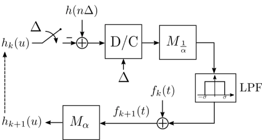
to lowpass filter it in order to produce a better approximation in the energy sense. In [42], it was proposed an extension of this algorithm through the inclusion of it-erative techniques, namely the itit-erative amplitude sampling reconstruction algorithm (IASR). Fig. 3-5 shows a block diagram illustration of the steps involved. The focus

(50)

Figure 3-5: Block diagram representation of the iterative amplitude sampling recon-struction (IASR) algorithm.

is placed on reconstructing the amplitude-time function ℎ from the uniform samples {ℎ(𝑛Δ)}_𝑛∈Z. Note that if the initialization satisfies ℎ0(𝑢) ≡ 0 and 𝑓0(𝑡) ≡ 0, the

first iteration corresponds precisely to the approximate recovery described above, i.e. 𝑓1(𝑡) = ˜𝑓 (𝑡). The objective is then that, iteratively, the error ||𝑒𝑘(𝑡)||2 is reduced.

We present simulation results in order to compare IASR against an iterative re-construction algorithm from nonuniform time samples. In particular, we consider the Voronoi method proposed in [25, Theorem 8.13], which presents the best perfor-mance, in terms of rate of convergence, among nonuniform sampling reconstruction techniques. Note that Theorem 3 is a generalization of the latter, i.e. it reduces to the Voronoi method whenever 𝑁 = 0.

We use noise bandlimited to 𝜎 rad/s and bounded by 𝐴 > 0 as input signals. Clearly, the slope for obtaining ℎ can always be chosen such that |𝛼| > 𝐴𝜎. From the discussion about sampling density in Appendix D, we set the parameters in such a way that Landau’s density criterion is always satisfied, which, in our case, takes the value 𝜋/𝜎. Moreover, it is clear from (3.20) that the conditions of the sampling instants for the Voronoi method are always satisfied for an appropriate choice of the parameters. As shown in Lemma (3), it is sufficient to choose

Δ |𝛼| − 𝐴𝜎 >

𝜋

Amplitude sampling for signal representation

Amplitude Sampling for Signal Representation

by

Pablo Martínez Nuevo

Ingeniero de Telecomunicación, University of Valladolid (2010)

M.S., Electrical Engineering, Columbia University (2012)

Submitted to the Department of Electrical Engineering and Computer

Science

in partial fulfillment of the requirements for the degree of

Doctor of Philosophy in Electrical Engineering and Computer Science

at the

MASSACHUSETTS INSTITUTE OF TECHNOLOGY

September 2016

c

○ Massachusetts Institute of Technology 2016. All rights reserved.

Author . . . .

Department of Electrical Engineering and Computer Science

August 30, 2016

Certified by . . . .

Alan V. Oppenheim

Ford Professor of Engineering

Thesis Supervisor

Accepted by . . . .

Professor Leslie A. Kolodziejski

Chairman, Department Committee on Graduate Theses

Amplitude Sampling for Signal Representation

by

Pablo Martínez Nuevo

Abstract

Acknowledgments

Contents

List of Figures

Chapter 1

Introduction

Chapter 2

Amplitude Sampling

2.1

Principle of Amplitude Sampling

2.2

Transformation by Ramp Addition

2.2.1

Mapping between 𝑓 and ℎ

2.2.2

The Sampling Process

2.2.3

Sampling Density

2.3

Spectral Properties

2.4

Decay Properties

2.4.1

Moderate Decrease

2.4.2

𝐿

norms

2.4.3

Slope Sensitivity

2.5

Summary

Chapter 3

Reconstruction in Amplitude

Sampling

3.1

Iterative Reconstruction Algorithms from

Nonuni-form Samples

3.2

Amplitude Sampling:

Recovery from

Nonuni-form Samples

3.3

Amplitude Sampling: Recovery from Uniform

Samples

3.3.1

Nonuniform Sampling of Nonbandlimited Signals

3.3.2

Approximate Recovery

3.3.3

Iterative Amplitude Sampling Reconstruction Algorithm

(IASR)