Analysis of bidding behavior of contractors in various economic conditions using utility assessment

(1)

ANALYSIS OF BIDDING BEHAVIOR OF CONTRACTORS

IN VARIOUS ECONOMIC CONDITIONS USING UTILITY ASSESSMENT by

ELIAS NICOLAS HANI

B.S., American University of Beirut (1974)

and YVES LESAGE

Ingenieur Civil, Ecole Nationale des Ponts et Chaussees (1974)

Submitted in partial fulfillment

of the requirements for the degree of Master of Science in Civil Engineering

at the

Massachusetts Institute of Technology

June, 1975

Signature of Coauthor

Department of Civil Engineering, May 20, 1975

Signature of Coauthor

Department of CilEngineering, May 20, 1975

Certified by

/

I

Thesis Supervisor

Accepted by

Chairman, Departmental Committee of Graduate Students

of the Department of Civil Engineering

(2)

ABSTRACT

ANALYSIS OF FIbBING BEHAVIOR OF CO 'TRACTORS

I) VARIOUS ECONOMIC CONDITIONS USING UTILITY ASSESSIhiENT by

ELIAS NICOLAS HANI and YVES LESAGE

Submitted to the Department of Civil Engineering on May 20, 1975 in partial fulfillment of the requirements for the

de-gree of Waster of Science in Civil Engineering.

Existing bidding strategies use expected monetary value as

the decision criterion to account for the behavior of gene-ral contractors in risky situations.

We show that this criterion has shortcomings and cannot ex-plain what is observed in real world bidding. The use of utility theory provides a better way of analysing the con-tractors' behavior.

The results show that the economic position of a firm and

the size of the project it bids on are two factors, amongst

others, which are taken into consideration in bidding,

fac-tors, that existing bidding strategies usually neglect.

Thesis Supervisor

Title

Richard de Neufville

Professor of Civil Engineering

(3)

-2-ACKNOWLEDGEMENT

We wish to thank our advisor, Professor Richard de Neufville, for his guidance and encouragements throughout this thesis. His many suggestions helped us to find our way through the difficulties of the subject and to bring this work to an

early conclusion. We would like to extend our thanks to the general contractors of the Boston area we interviewed for their helpful cooperation. We are also grateful to the

staff of the Bureau of Building Construction and the Depart-ment of Public Works who helped us in collecting the data.

The authors wish to thank respectively the Lebanese National Council for Scientific Research and the French Ministry of Foreign Affairs for their financial support.

Special thanks go to Mrs Christiane Hani for the numerous sacrifices she has made.

(4)

-3--TABLE OF CONTENTS Page Title page 1 Abstract 2 Acknowledgement 3 Table of contents

4

List of tables ₈ List of figures ₁₀ 1. Introduction

1.1 Statement of the problem 12

1.2 Bidding strategies and utility theory 13

1.3 Organization of the study 15

2. A review of the literature of bidding strategies 17

2.1 Introduction 17

2.2 The general model ₁₈

2.3 State of the art 22

2.3.1 Objectives 22

2.3.2 Profit ₂₃

2.3.3 Probability of beating a given 25

competitor

2.3.4 _{Probability of beating a number of} ₂₇ competitors

2.3.5 Refinements 30

2.4 Other strategies ₃₁

(5)

Page

2.5 Conclusion ₃₃

3. Utility theory and assessment ₃₈

3.1 Introduction ₃₈

3.2 Utility ₃₉

3.2.1 Expected utility ₃₉

3.2.2 _{Selling and buying price of a lottery} ₄₀ 3.2.3 Properties of utility functions 42 3.2.4 Risk premium and risk behavior

₄₇

3.3 Utility assessment L9

3.4 Conclusion ₅₁

4.

Data analysis ₅₃

4.1 Gathering data ₅₃

4.2 _{Comparison of the number of bids per year} ₅₄ with the yearly allocated award

4.3

Number of bidders per project 58

4.4 Deviation from estimate 62

5. Utility assessment ₆₇

5.1 Introduction ₆₇

5.2 _{Development of the questionnaire} ₆₈

5.2.1 General considerations 68

5.2.2 Types of questions 69

5.2.3 Final form of the questionnaire ₇₅ 5.3 Utility assessment and results 77

(6)

-5-Page

5.3.1 From theory to practice 77

5.3.2 Treatment of data 79

5.3.3 Results 82

5.4 Conclusion 84

6. Comparison of results 85

6.1 Introduction 85

6.2 Interpretation of the results of the 85

utility assessment

6.2.1 Certain cost situation 85 6.2.1.1 Normal size of jobs 86

6.2.1.2 Large size of jobs 91

6.2.2 Uncertain cost situation

94

6.2.2.1 Normal size of jobs 96

6.2.2.2 Large size of jobs 97

6.2.2.3 Illustration 97 6.3 Comparison of results 100 6.3.1 Predicted behavior 100 6.3.2 Actual behavior 107 6.4 Conclusion 109 7. Conclusion 110 References 114

Appendix A Tables of data analysis 117

Appendix B Tables of utility assessment 127

(7)

-6-Page

Appendix C Tables of comparison of results 131

Appendix D Questionnaire 140

(8)

LIST OF TABLES

Page

6.1 Variations in the degree of risk aversion, 92

certain cost case

6.2 Variations in the degree of risk aversion, 99

uncertain cost case

Al BBC data, main features 118

A2 DPW data, main features 119

A5 Number of projects versus average number 120 of bidders per project - BBC

-A4 Number of projects versus average number of 121 bidders per project - 3PW

-A5 Deviation of bids from estimated cost for 123

BBC

(

of estimated cost)

A6 Deviation of bids from estimate for DPW 124

(f

of estimated cost)

AT Deviation of bids from estimate for DPW 125 (/ of estimated cost)

AS Coefficients a and b found by linear 126

regression

B1 Assessed utility function 128

B2 Minimum rate of return 130

for the various contractors interviewed

(% return)

C1 Optimum markup for contractor 1 on normal 132

size of jobs, uncertain cost situation

C2 Optimum markup for contractor 1 on large 133

size of jobs, uncertain cost situation

(9)

-8-C3

Cumulative distribution function (C.C.D.F) 134 for 3 competitors - markup in percentage

-c4 Cumulative distribution function (C.C.D.F) 135 for

4

competitors - marKup in percentage

-C5

Cumulative distribution function (C.C.D.F)

136

-for 5 competitors - markup in percentage

-C6

Cumulative distribution function (C.C.D.F)

137

for 6 competitors - markup in percentage

-C7

Optimum markups for contractor

1,

138 certain cost situation,

using expected utility and monetary values

C8

Optimum markups for contractor 1,

139 certain cost situation

using expected utility and monetary values

(10)

-9-LIST OF FIGURES

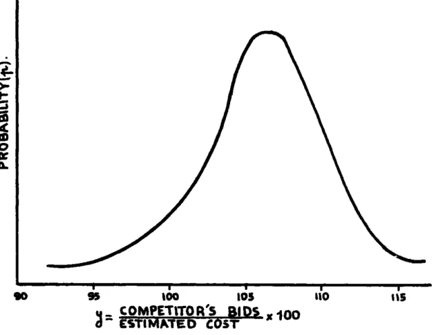
Page 2.1 Probability distribution of the ratio of 20

competitors bids over estimated cost

2.2 Expected profits 21

2.3 Optimum markup versus number of competitors 36

3.1 Example of utility function of a contractor

45

on a

$1,000,000

job - 0 U(x) 1

-3.2 Example of utility function of a contractor 46 on a $1,000,000 _job _- ₅_< V(x) _{< 15}

-3.3 Characteristic shapes of utility curves 48 4.1 Amount of money awarded and number of 56

projects awarded per year versus year (BBC)

4.2 Amount of money awarded and number of 57

projects awarded per year versus year (DPW)

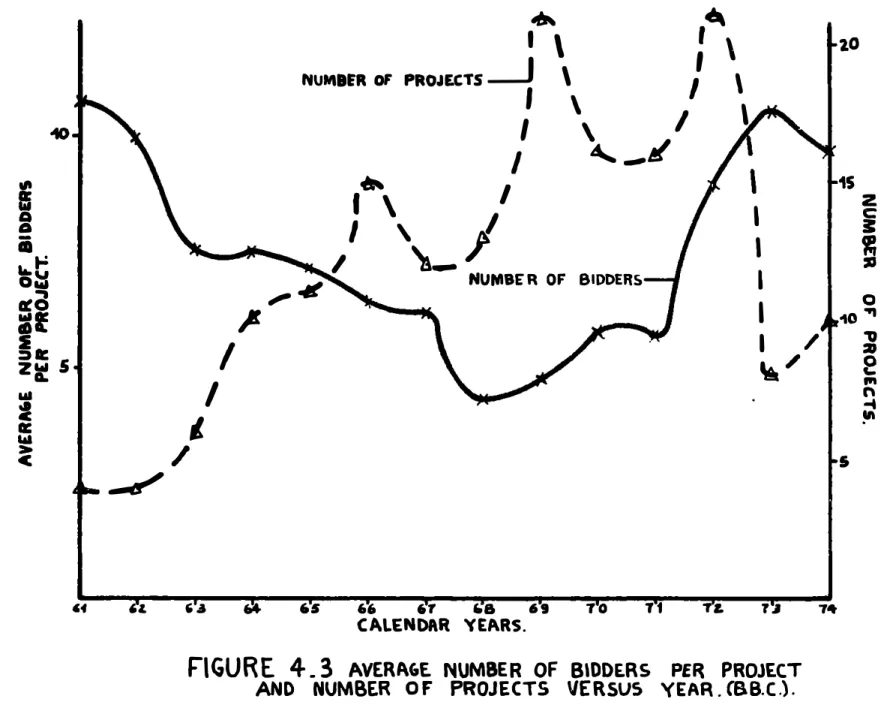
4.3 Average number of bidders per project and 59

number of projects versus year (BBC)

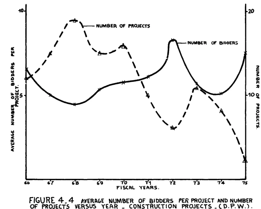
4.4 Average number of bidders per project and 60

number of projects versus year construction projects (DPW)

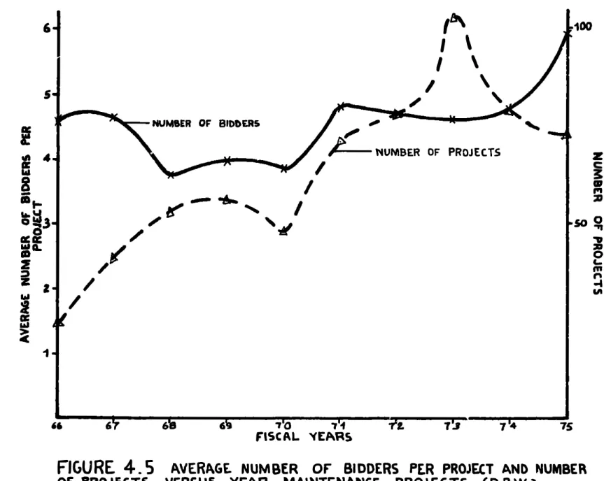
4.5

Average number of bidders per project and 61

number of projects versus year maintenance projects (DPW)

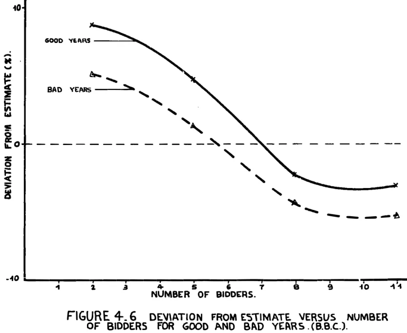
4.6 Deviation from estimAte versus number of 63

bidders for good and bad years (BBC)

4.7 Deviation from estimate versus number of 66

bidders for 1967, 1969, 1971, 1973

6.1 Utility functions given certain cost and 87 normal size of job

6.2 Plot of the ratio, w(x), of utilities in bad 89

and good times

(11)

6.4 Utility functions given certain cost and

93

large size of job

6.5

Complementary cumulative distribution 101 function for 3 competitors

6.6 Complementary cumulative distribution 102

function for 4 competitors

6.7 Complementary cumulative distribution

103 function for

5 competitors

6.8 Complementary cumulative distribution

104 function for 6 competitors

6.9 Optimum markups for contractor 1, certain

106

cost situation, using expected utilities

and monetary

values, cost

=

0.95 EE

6.1o Optimum markups for contractor 1, certain 108 cost situation, using expected utilities

and monetary values, cost = 0.97 EE

(12)

-CHAPTER 1

INTRODUCTION

1.1. Statementof the problem

All firms in the construction industry have had to resort to

closed competitive bidding as a means for getting work. A

contractor is given a set of plans and specifications and is requested to submit in a sealed envelope his bid, or the price for which he agrees to do the work. The contractor takes many factors into account before submitting his bid: he considers the competition on the job, the type of work

involved, his need for work, his financial status, the re-quirements of the job in men, materials and equipment, the availability of those, the size of the job, its risk, the overhead involved, etc... He then relies on his judgment and experience to submit his final bid. This bid will be based on his cost estimate increased by a certain percen-tage, called the markup, which allows for profit, overhead and contingencies. If his markup is too low, he will get the job but he will either lose money on the job, or get a very low return on investment and thus he will barely be able to survive. Usually the only difference between a flourishing company and another on the edge of bankruptcy

(13)

in time.

One of the contractor's most important decisions is what optimum markup will insure maximum profits in the long run together with a good level of return on investment. This decision problem which faces the contractor can therefore be described as follows. After the contractor estimates the cost of the job he has to decide on the markup to be added, which can be any value between two extreme limits (usually 2% to 15%); then he has to observe what we call the state of nature, or the lowest bid among his competitors. If his bid

is higher he will not get the job and will have lost the money spent on estimating the work which usually ranges between 0.5 to 2.0 percent of the total project cost. On

the other hand, if his bid is the lowest, he will get the job and will end up after the execution of the work with a profit (or loss) equal to his markup minus job overhead minus variation in cost from the estimate. At the same

time he suffers an opportunity loss which is the difference between his bid and the second lowest bid; this is referred

to as the money left on the table, or the spread.

1.2. Bidding strategies and utility theory

To help the contractor determine the optimum markup, compe-titive bidding strategies have been developed by several

(14)

-13-investigators. A strategy can be defined in a number of different ways, but perhaps the most suitable definition for our purposes is: A bidding strategy is the science and art of meeting competition under the most advantageous condi-tions possible in order to achieve a certain goal.

The problem we face can be stated in the following manner: Are these mathematical formulations of a fairly complex

situation realistic enough to be applied in practice? Are the assumptions on which they are based justified? Is the actual behavior of contractors in real situations consis-tent with what is predicted by these strategies? In fact all bidding models considered that the contractors have expected monetary preferences, and that the number of bid-ders and the probability of winning are the major factors influencing the bid price. These factors can be repre-sented schematically as follows:

NUMBER OF BIDDERS

(15)

where C.C.D.F is the complementary distribution function of the density distribution of markups: it gives the probabi-lity of winning given a certain markup.

However we feel in this study that the decision-makers have expected utility preferences, and that some other factors, like the relative size of the project and the economic

situation ("good" or "bad" times), are also of major influ-ence. _{We suggest the alternative representation:}

ECONOMIC CONDITIONS SIZE OF PROJECT

[NUIMBER OF BIDDERSUTILITYJ

C.D.F BID PRIC

1.3. Organization of the study

The second chaper of this study reviews the state of the art in 1975 concerning bidding strategies. It first intro-duces the basic idea common to all the models, and then discusses the sometimes contradicting refinements or

(16)

-assumptions considered in the different strategies. The expected monetary value criterion which constitutes the

basic principle of all the models is criticized in chapter 3 and the invalidity of such a criterion is shown. The same chapter also introduces the utility theory which was deve-loped to deal more efficiently with uncertain situations. The next step is then to analyse actual behavior in bidding situations, in order to verify the validity of the expected utility criterion. The results of the analysis of public bids collected from two state agencies are presented in chapter

4.

Chapter 5 is concerned with the development of a questionnaire for assessing the utility functions of some contractors in the Boston area. The factors influencing the utility functions are first determined, then the ques-tions used and their interpretation in terms of the utility functions are considered. We finally discuss the diffi-culties encountered in the actual assessment, as well as the results obtained. Chapter 6 presents the interpretation of the assessed utility functions, followed by a correlation between the predicted behavior, obtained through the utility functions, and the measured behavior from public bids. This exposes the deficiency in the existing bidding strategies. The conclusion suggests some possible extensions of this study for future research.

(17)

-CHAPTER 2

A REVIEW OF THE LITERATURE OF BIDDING STRATEGIES

2.1. Introduction

Numerous bidding strategies have been developed to apply to different kinds of situations. They can be classified

according to whether they are concerned with:

(1) Determining the optimal bid for a single job.

(2) Sequential bidding, that is, simultaneous bidding on more than one contract.

(3) Situations involving lump-sum bids.

(4)

Unbalanced bidding on unit price contracts.

Although most of the strategies deal with bidding against competitors, some of them also deal with bidding against the owner.

This study focuses on non-sequential closed competitive bid-ding on lump-sum contracts, since most other bidbid-ding

situa-tions can be considered as extensions of this basic model. Almost all of the existing bidding strategies more or less follow the first bidding model, developed by Friedman (1956) for the oil industry. But many of the assumptions change, sometimes significantly, between different models. Fur-thermore each model considers different factors that,

(18)

-according to the author, significantly affect the optimum bid, factors that are not considered or even are rejected

by other models. The general contractor who is the poten-tial user of such models should be aware of the weaknesses (present in the assumptions) involved in any specific model before he decides to use it.

We review and present the different bidding strategies cur-rently available for use in the construction industry as follows: first the basic general model common to almost all strategies; secondly, and in some detail, all known devia-tions ar elaboradevia-tions around this model; finally, some of the models which differ significantly from the basic idea of the general model. This part is based on the study of dif-ferent bidding models developed by Friedman (1956), Park

(1966), Gates (1967), Morin and Clough (1969), Shaffer and

Micheau (1971), which generally represent the state of the art in 1975.

2.2. The general model

The general model supposes that the objective of the com-pany is to maximize the total expected profits, given by

the general formula:

E(P)

=

p(P) x P where E(P) is the expected profit

(19)

-P is the profit (or markup) included in the bid price p(P) is the probability of being the low bidder given a profit P.

Based on past bidding data the probability p (P) of beating competitor i given P can be determined. This is done by developing bidding patterns for the different competitors. Given competitor i's bids on past projects, a frequency distribution of the ratio of com₁ _{etitor's bids as a percent} of estimated cost can be plotted and a probability distri-bution function can be fitted (see figure 2.1). Then, for any given P, pi(P) can be found: it is the complementary distribution function (C.C.D.F)

Pi(P)= 1

-J

p dy

If there are n competitors the probabilities of beating each one individually are combined in a certain way (discussed later in this study) to give the probability p(P) of beating them all given a certain profit level P. E(P) is then

plotted versus P (expressed as a percentage of the estimated cost of the work) and the optimum profit P0 can be deter-mined. (see figure 2.2)

However there are significant deviations between the dif-ferent strategies on the following points:

1) _{What is to be considered as profit.}

(20)

-

>-C

0

so too 105 It'O 's

COMPETITOR'S BIDS xlOO

ESTIMATED COST

FIGURE

2.1 PROBABIMITY

DISTRIBUTION OF THE

RATIO Of COMPETITORS BIDS OVER ESTIMATED COST.

(21)

20-tlog

L

La

VI Ll

FIGURE

2.2 EXPECTED PROFITS.

(22)

-2) How to obtain the probability of beating a given compe-titor.

3) How to combine the n individual probabilities in order to obtain the probability of beating the n competitors.

4) How to treat the individual competitors when their iden-tity is either known or unknown.

5) How to deal with the case when the number of competitors is unknown.

In addition to the above mentionned points, which can be considered to have a direct relation to the general model,

some other factors are introduced by different models and have a direct influence on the optimum markup. These in-clude the following: the class of the work, its size and contingencies.

2.3. State of the art 2.3.1. Objectives

The assumptions and deviations between the different stra-tegies will be presented in the same order as mentionned above. It is obvious that the optimum markup depends pri-marly on the objectives of the company. In the case of the

construction industry there are many possible objectives: 1) Maximize total expected profit

(23)

2) Maintain a prescribed level of return on investment.

3) Minimize expected losses (during idle periods).

4) Minimize competitors' profits to maintain competitive position.

5) Keep a certain share of the market.

6) Increase volume of work as much as possible.

7) Increase volume of work to keep up with inflation only. 8) Try to maintain labor force at work at any cost.

Almost all of the bidding strategies developed until now have the objective of maximizing total expected profit

(which is most common). But, for example, if a company's objective is to maintain its labor force, its optimum markup can well be negative. The user of bidding models should be aware of this basic assumption of maximization of expected profits which is the foundation of all the strategies.

2.3.2. Profit

The profit P on a certain job can be considered to be equal to B - Ca - OH where B is the bid price, Ca the actual cost of contruction and OH the overhead. Both Park (1966) and Gates (1967) assume in their models that profit is equal to the bid price (B) minus the estimated cost of construction

(Ce). No consideration is given to overhead which is as-sumed to be included in the cost estimate and no correction is introduced to adjust for the fact that in actual cases

(24)

-23-the cost of construction is different from -23-the cost estimate. Gates recognizes this difference and contends that it is

small enough to be neglected. He also suggested a correc-tion for bias in a brief explanacorrec-tion of break-even analysis. Similarly, Friedman (1956) assumed that overhead is included in the cost estimate but he considered profit to be the dif-ference between the estimated cost of fulfilling the con-tract corrected for bias and the bid amount. He suggests that one can develop, through a study of past data on esti-mates and actual costs, a probability distribution of the true cost as a fraction of the estimated cost. Letting S be the ratio of true cost to estimated cost (0

),

B the amount bid for the contract, p(B) the probability that a bid B will be the lowest and winn, then the expected profit suggested by Friedman will be:

E(P)

=

p(B) B - S C3 h(S) dS

where h(S) is the probability of a certain S. Alternatively

E(P)

=

p(B)

[B

-

C']

ca

where C'

jS

h(S) dS and is the expected actual cost. On the other hand, iorin and Clough (1969) assert that the

expected actual cost will equal the estimated cost. They found, from the study of data for a certain company, that

(25)

the ratio of actual to estimated cost approached a symme-trical distribution with a median of 1.0 and a standard

deviation of less than 2%. But, unlike the previous models, they recognized the fact that overhead actually differs

significantly from one company to another. So the profit to be maximize is the net profit which is the difference between the markup (MP) and the overhead (OH):

E(P)

=

(MP

- OH) p(MP)

where p(WLP) is the probability of being the low bidder with a markup of MP.

2.3.3. Probability of beating a given competitor

To determine the probability of beating a known competitor, all models suggest that one should study past bidding data and develop (in different ways) a probability function for the ratio of the competitor's bid to our estimated cost.

Friedman (1956) and Park (1966) suggest fitting a continuous probability function to the available data; Casey and

Shaffer (1964), a normal distribution function; Gates (1967) uses on the other hand a statistical linear regression to determine this probability and expresses the profit P as:

P = a logpi- b

where pi is the probability of beating competitor i given

(26)

-a profit P. a and b are determined from the plot of P versus log pi for all past bidding data.

When the identity of the competitor is unknown or when insufficient data are available to develop the probability functions, all the above models combine past data to get a general bidding pattern for a typical competitor.

The OPBID model of Morin and Clough varies significantly from the other models. First they felt that recent data

should receive more weight than older data because the-com-petitive situation changes with time, they suggested using

an exponential weighting scheme; secondly they classified competitors as being either key or average, depending on the percentage of past biddings they participated in. If this percentage is greater than a certain specified ratio (0.4 to 0.5 was suggested) the competitor is classified as key com-petitor, if it is lower the competitor is considered as ave-rage. The advantage of this classification is that it is a weighting scheme in which companies competing on a relati-vely large number of jobs are given much more attention than occasional competitors. Finally in order to assess the pro-bability of winning with a given bid, the OPBID model uses a discrete probability distribution which has the following

three advantages:

1) It eliminates errors introduced by fitting smooth

(27)

26-probability curves to existing data.

2) It permits fast calcutions by a digital computer

3) It provides a general model that can be used by dif-ferent contractors.

2.344. Probability of beating a number of competitors

Given that the number n of competitors on a certain project

is known and given the probability pi(B), all models follow

more or less one of two methods to determine the probability of beating the n competitors.

Some of the authors (Clough, Friedman, Park) assume that the probability of beating any given competitor is independent of that of beating any other competitor, and therefore the probability of beating them all is the product of the indi-vidual probabilities.

Pn(B)

=

iT

P(B)

pn (B) is the probability of winning over the n competitors given a bid price B.

In the.case of Clough's model this probability is:

N'

pn(B) = [TTN p(B

)I

a(B) av

key

j~

v

where n can be subdivided in Nkey competitors and N'

ave-rage competitors.

(28)

-When the identity of the competitors is not known the

proba-bility of winning becomes:

Pn(B)

₌

_Pav(B)]"

The second method, developed by Gates, rejects the idea of the probabilities of beating individual competitors being statiscally independent, and contends that when you beat a certain competitor you will revise your estimate of beating the others. The probability of winning becomes:

Pn(B)= ; ;B)

F. I- )i () +1

n pi(B)I

When the identity of the competitors is not known is sim-plifies to the following:

PnB)=n p (B)

n (1 -p ay(B)) + 1

Broemser (1968) developed and used another method in his model. He dissociates the probability of winning from the number of competitors on a given job and contends that it is sufficient to beat the lowest bidder. So, using past data, he determines the distribution of ra, the ratio of the

lowest competitor's bid to the estimated cost, by a linear regression which attempts to explain the behavior of the

(29)

-28-low competitor by certain requirements of the particular

job. _{These include estimates of the percent of cost not}

subcontracted, the duration of the job, the ratio of job duration to estimated cost, and the cost. This model tries to go around the problem of determining the probability of beating n competitors by implicitly assuming a certain rela-tion between the number of competitors and the characte-ristics of the job.

When the number of competitors is unknown the different strategies use different ways to predict this number. In his original work, Friedman suggested the use of one of two methods:

1) _{The number of competitors might be given by a Poisson} distribution whose parameters are determined from tests of past data.

2) _{A linear regression is used on past data of number of} bidders against the cost estimate of the contract. He

assumes that the larger the size of the contract, the higher the number of competitors.

Similarly Park assumes that the number of competitors is a function of the job size, and that this number increases until a certain limit job size then decreases for larger sizes.

On the other hand, Gates as well as Morin and Clough

(30)

-suggests using the mean of the number of competitors encoun-tered on previous biddings,since, using real world data they could not come up with a relation similar to that suggested

by Friedman and Park. 2.3.5. Refinements

Some other refinements were introduced by some bidding models. These concern the class and size of the work as well as contingencies. Morin and Clough suggested the

clas-sification of historical data in different "classes of work" since the chances of winning with a certain markup on one class of work might be different from the chances of winning with the same markup on a different class of work due to the variability of risks involved or the time required for

exe-cution. Park suggested an interesting extension for his bidding model. He recognized that the optimum mark up

de-pends on the size of the job, the larger the job, the lower the optimum markup, and suggests the following relationship:

x

[Coil

MP

₂

where Co is the estimated direct cost on job 1, and LP1 the

optimum markup on job 1. The exponent x can be determined from the bidding history and he proposes a value of 0.2 in his article.

(31)

As far as contingencies are concerned Gates (1971) catego-rized contingencies into four groups: mistakes, subjective uncertainties, ojective uncertainties, and chance variations. He dealt with such problems as mistakes of omission, pro-blem of natural events, production rates etc... and he used

analytical methods based on statistics and probability to obtain for each case likelihood of occurence, costs and fi-nally expectation values.

2.4. Other strategies

This section presents two models which significantly vary from the fundamental idea of the general bidding model. The first is the "least bidding strategy" developed by Gates and the second is the strategy proposed by Shaffer and Micheau (1971).

The "least bidding strategy" is based on Gates' finding that the average spread ( Ba) is a function of the size (C) of

av

the low bid. Specifically he came up with the following expression:

Bay

=

1.08 CO.734

He also found in his original study that 67P" _'

Ba- 1-(p)

(32)

-where P' is the amount to be added to the completed bid and

(p) the probability of still being the low bidder after in-creasing the bid by P'.

Using these relations and assuming that you were 100o cer-tain (relatively) that for your initial bid B you would be the low bidder, Gates determined the optimum amount P' to add to your bid to maximize your expected profit. This is given by:

P',= 0.80 C 0 '34 -

0.50

B

It is interesting to note at this point that a similar rela-tion was found by Park relating the percent average spread to the number of bidders and he suggests a linear relation: the higher the number of bidders the smaller the average spread, but he did not pursue his idea further.

All the models presented until this point rely only on

ma-thematicals expressions using past bidding data, and the contractor had only to input his information into the model to come up with an optimum bid. An extension of previous models was presented by Shaffer and Micheau (1971) who reco-gnized that too many variables influence actually the selec-tion of an optimum bid, that no model took all of these into consideration, and that judgment based on experience can be of great value in arriving at a final choice of a bid. So they suggested a combination of formal and informal means,

(33)

with the formal means being competitive strategy models and the informal means being personal judgment of the contractor. The whole object was to determine with the formal means an upper and a lower bound to provide the contractor with a focus- for his judgment. The actual selection of the bid would be obtained solely by informal means, the lower bound of the range would be the bid that would give the contractor the greatest chance of submitting the low bid for the

pro-ject and the upper bound would be the bid that would give him the greatest chance of submitting the second low-bid.

Shaffer and lMicheau also recognized the fact that different bidding models apply best to different situations and that a person cannot a priori decide that this particular bidding strategy will apply best to all companies or to a particular company. So they recommend to select a few strategies and to test these using past bidding data and then the models to be used to determine the upper and lower bound will be those whose results have had the greatest success on historical data of yielding the low and second low bids respectively.

2.5. Conclusion

Although most of the strategies follow the same basic idea presented in the general model, apparent large differences

exist in many of the fundamental points considered. These

(34)

-33-points of disagreement can be restricted to two major ones:

1) What is profit.

2) How to get the combined probability of winning.

As far as profit is concerned, some models assumed the ac-tual cost to be equal to the estimated cost and most of the models did not consider overhead which affects obviously the probability of winning. However this disagreement is mostly

superficial. As regards the correction for bias of the es-timated cost, it is safe to assume that the estimator, based on a knowledge of his past performance, will continuously adjust his method for computing the estimate to account for the bias that has occured in the past; there will then be no need to correct for bias. Consider on the other hand the

overhead; if it is accounted for in the cost estimate (as assumed in most strategies) and is high, the probability of winning for a given markup will be lower than when the over-head is low for the same markup. However if the overhead of a certain company did not fluctuate much in past bids and is still at the same level, one can affirm that this overhead would have influenced the "bidding patterns" developed for

the competitors and no other correction is required.

As far as the probability of winning against a number of

competitors is concerned, numerous articles and discussions were written to support either of the two assumptions

pre-sented by Friedman and Gates - Stark (1968), Baumgarten

34

(35)

(1970), Benjamin (1970), Naykki (1973), Dixie (1974) - while other articles tried to reconcile them - Rosenshine (1972) -All the strategies agreed, however, on the fact that the

higher the number of competitors, the lower the probability of winning and therefore the lower, the optimum markup (see figure 2.3).

Nearly all of the models presented developed or introduced certain relations between the different variables, and cer-tain factors which they considered would have an effect on

the optimum bid. But as suggested by Benjamin Neal (1972) the weaknesses and the disagreements between the different models may be due to the fact that they use single variable

statistical techniques to deal with a situation which is ac-tually much more complex.

Although there is much controversy between the different bidding models studied in this part, all agreed on the basic assumption of maximization of total expected profits. They all implicitly assume that people behave in a specific way, behavior which may not be observed in real world situations. To consider that people actually decide according to

expec-ted monetary value may be a major weakness. Although this is the subject of the next chapter, a simple example illus-trates this point: if a person behaved consistently with

the above assumption then he should be indifferent between participating to a lottery offering an equal chance of

(36)

-0!

0

HUM13ER OF COMPETITORS.

FIGURE

Z..

3 opTimum MARKUP

VER.Sus

NUMBER OF COMPETITORS .

(37)

-36-gaining or losing $10,000, or not participating at all. But in fact most, if not all, people will not even consider such a lottery. The fact that all models do not account for the effect of various economic conditions on the optimum bid is one aspect of this weakness. All available bidding

stra-tegies indicate that the contractor should add the same markup for a given project, regardless of the economic con-ditions. In fact, one might expect that in bad economic conditions the bids will be lower: the contractors are much more interested in winning the contract due to the fact that they are more in need for work than in normal times. Other aspects of the weakness of the models will be discussed

later on, in this study.

The next step is therefore to introduce a criterion, expec-ted utility value, that would do away with the weakness of

the expected monetary value criterion. We then determine through an analysis of actual bidding data the behavior of the contractors in various economic conditions. The aim is to test the validity of the existing models and of the ex-pected utility value criterion to determine if its use gives consistent results with observed real world behavior.

(38)

CHAPTER 3

UTILITY THEORY AND ASSESSMENT

3.1. Introduction

The review of various models of bidding strategies in the literature shows that all of them deal with expected mone-tary value as a decision criterion. This makes implicit assumptions which may bias the evaluation of a bid, and lead to erroneous conclusions. The first assumption is that a unit of loss has the same value as a unit of gain, i.e. that a contractor should be indifferent between

staying in his present situation and having a lottery where

he can lose $A with a probability of .5 or win $A with a probability of

.5.

That may be true if A equals $1 or $10

but if the amount of money goes to $10,000 or $100,000 the contractor may think he is better off away from that gamble. The fact is that people generally give more weight to

losses than to gains, and taking expected monetary value does not take into account the spread of the outcomes.

The size of the loss that one can afford mainly depends upon one's assets. For instance a small contractor might not be willing to bid on a risky $10,000,000 job, because if it

fails, he may go bankrupt. On the other hand a bigger

-

(39)

38-company may take it, for, in the worst case it may run into a cash problem. However, if the small company is at the point where it needs a high gain to avoid bankruptcy, it might take the project on the grounds that if it fails the bankruptcy will only be a little worse, whereas if it

suc-ceeds, it will not go bankrupt at all. All these factors

are not taken into account by the expected monetary value criterion, for it makes the assumption that everyone shares the same values for all items at all times. These various difficulties encountered in using this criterion can be cleared up by the use of a recently developed tool of deci-sion analysis : utility theory.

3.2. Utility

3.2.1. Expected utility

Given a certetit number of axioms, which we will discuss later, a utility function can be defined as the

represen-tation of a set of numbers which are generated for each

possible outcome of a decision, numbers which can be used to order all choices according to their desirability to the decision-maker.

An outcome can be represented by a vector of attributes. In this study we will only be concerned with utility func-tions with one attribute. Such functions scale preferences

(40)

-for the attribute - in this case, the percentage of markup on a project. Instead of working with expected monetary values we will use expected utility value. This criterion

enables us to compare two possible decisions, knowing the various values of the attribute which result from the

deci-sions. We proceed in the following manner : letting U(x) be the utility function of a contractor, the expected value of

the utility EUV of a decision is EUV

=

En

U(x)

where x. is the value of the attribute corresponding to one of the n possible outcomes of the decision, and p. the pro-bability of occurence of this outcome. To compare two deci-sions, one compares their two expected utility values, and chooses the decision with the maximum expected utility.

3.2.2. Selling and buying price of a lotters

Suppose that you own a lottery ticket which gives you a 50-50 chance of winning $1000 or $0, and that we ask you to sell that ticket for $300. Must you accept ? Such a deci-sion can be represented by (Raiffa 1968)

(41)

$300 $1000 decision node chance node $0 lottery

If you are indifferent between the two choices, $300 is

said to be the certainty equivalent of the lottery ($1000, .5 ; $0, .5). This can be represented by

$1000

$300

-'too

<

$0

If two choices are equivalent their respective expected

utility values are equal. We can write

1 x U($300) = .5 x U($1000) + .5 x U($0)

(42)

-$300 is said to be the selling price of such a lottery.

We can consider another type of lottery corresponding to the following question : how much would you pay to have a 50-50 chance of winning $1000 ? This can be represented by

$1000 - b 0

$0

.4

- b

where b is the amount you would pay. b is said to be the buying price of the lottery.

3.2.3. Properties of utility functions

Very often a utility function is monotonic. For instance if the attribute is the profit on a project, more is better the utility function is monotonically increasing.

If the utility of a decision is twice the utility of another decision, it does not mean that the results of the former decision will be twice as good. The function has ordinal properties and not cardinal ones, it works exactly as

temperature scaling. You can compare two temperatures and say that one day is hotter ot colder than another one ; nevertheless, one cannot say that a given day with a tempe-rature of 60"F is twice as hot as another with a 30F

(43)

You can take a linear transformation of the utility function U(x), which transforms U(x) into V(x) = a U(x) +b (a>0), without changing the relative ranking of the decisions ;

that is exactly what happens when temperature is expressed in degrees centigrade instead of degrees Farenheit. In

that case U(x) and V(x) are said to be strategically

equivalent.

A utility function is defined on a certain range which is

meaningful to the person whose utility function is assessed. For instance it is meaningless for a general contractor to consider a 50% profit on a project, because he could never reach that. Therefore the range of definition of a utility function should cover all the values of the attribute which

can be considered in any decision-making process. Then two

utility values are assigned to two different outcomes (as 326F and 212*F are respectively assigned to freezing point and boiling point of water). Usually the values 0 and 1 are respectively given to the lowest and highest value in the range considered. In the following example, which illus-trates what we have said about utility functions until now, we consider a range of profit going from -5% to 10%. We

assume that the worst thing which can happen on the project is a loss of 5% and the best thing is a profit of 10%.

(44)

43-In figure 3.1 we can see the following correspondance

x

-5%

-1% 2% 10%

U(X) 0 .5.75 1

In figure 3.2 we have another correspondance

x

-5%

-1% 2% 10%

V(x)

5

10

12.5

15

It is easy to see that

V(x) = 10 U(x) + 5

Using these curves, let us find the certainty equivalent of the following lottery :

-1% profit

$0

10% profit

Let us first compute the expected utility value U(x)

U(x)

=

.5

U(-1%)

+ .5

u(i0%)

(45)

4. 'C

5

I I., - - -- - - I

r

-g I I

F

I I I I I I I I

I

I I I I 1 I I * -4

e~6

4

10 MARKUP C

V.

OF COST)

FIGURE 3~1

EAMPLL OF UTILITY FUNCTION OF

A

CONTRACTOR ON A

$

IPOQOOO JOB

-

0 ~ V(fl141

(46)

"i

MAKU( OFCOT

5IUE3

XML

F TLT

UCINO

(47)

We conclude from figure 3.1 that x equals 2%. Let us

compute the expected utility value V(x) :

V(x) = .5 V(-i%) + .5 V(10%)

.5 x 10 + .5 x 15

=

12.5

From figure 3.2, we conclude that x equals 2%. As expected the answer obtained with V(x) is the same as the one

obtained with U(x), since the two are strategically equivalent.

3.2.4. Risk premium and risk behavior

The risk premium is defined as the difference between the expected monetary value and the certainty equivalent. In the above example we found that the certainty equivalent

was 2%o. The expected value is :

.5 X 10% +.5 x -1%

=

4.5%

The risk premium r equals :

r

=

4.5%

-

2%

=

2.5%

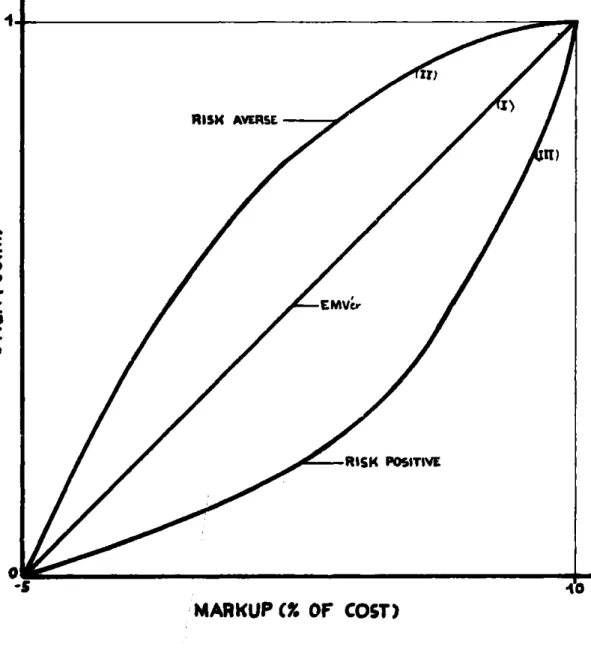
If the risk premium is positive, the decision-maker is said to be risk-averse. In case of a negative risk premium he is said to be risk-positive. If the risk premium is equal to zero, he is said to be an EMV'er. Figure 3.3 shows the three characteristic shapes of utility curves. Curve I

(48)

rp I) RISK AVERSE Kr) x '.9 EMVir RISK POSITIVE

MARKUP CZ OF COST)

(49)

represents the utility curve of a decision-maker who decides according to expected monetary value over the whole range. Curves II and III respectively represent risk-averse and

risk-positive behavior over the whole range.

It is often interesting to measure risk-aversion, and to be able to say that a decision-maker is more or less risk-averse than another. The risk premium is not a good mea-sure when the range of the utility function is changed. Pratt (1964) showed that if U(x) is the utility function,

the ratio r(x) = - U"(x) / U'(x) gives a good measure of risk-aversion. It is easy to see that r(x) is identical

for two strategically equivalent utility functions.

As was said earlier, the existence and properties of uti-lity functions are based on a certain number of axioms. One of them deserves some special attention, because of the

criticism it receives. It is the transitivity of prefe-rences : if you prefer outcome A to outcome B and B to C you must prefer A to C. Raiffa (1968) shows that somebody who has an intransitive behavior is bound to lose all his

assets to someone who adequately uses this intransitivity.

3.3. Utility assessment

To use the expected utility criterion in the bidding stra-tegy of a contractor, you need to assess his utility

(50)

function. Such assessments have been made in other fields: Grayson (1960) made a study of oil wildcatters, Swalm (1966) and Spetzler (1968) of business executives, Lorange and

Norman (1970) of shipowners, de Neufville and Keeney (1971) of executives of the Mexican Ministry of Public Works and Willenbrock (1973) of contractors. In all these studies, the interview method was used to assess utility functions; a discussion of the validity of such a procedure is made by Lorange and Norman (1970).

The type o0 questions asked in any of the interviews is as follows: For what amount of money will you be indifferent between I and the following lottery?

XX

X2

In this lottery you can win _X1 _{with probability p and}_X2

with probability 1-p. Answers to a certain number of these questions enable the interviewer to draw the utility

func-tions of the decision-maker. Two procedures can be used to

obtain these curves. One is to let X1 and X2 be fixed and to vary p; we call this the constant-attribute procedure.

The other is to let p be fixed - generally equal to .5

-and vary X11 and X2; we call this the constant-probality

(51)

-procedure.

Grayson (1960) and Spetzler (1968) used the

constant-attribute procedure. Swalm (1966), de Neufville and Keeney (1971) and #illenbrock (1973) used the constant-probability procedure. Lorange and Norman (1970) used both procedures. These studies show that the persons interviewed have pro-blems in dealing with probabilities different from

.5.

Grayson (1960) writes:

"Probabilities created the greatest difficulty in the experiment. Some operators do not normally

use numerical probabilities in their decisions,

and they found it strange to try to reach a deci-sion on the basis of probabilities."

In Lorange and Norman's study this problem was reflected by the fact that shipowners were significantly more risk-averse vis-a-vis attribute gambles than versus

constant-probability gambles.

Both assessment procedures discussed above are valid, but the constant-probability one is more suitable because more easily understood by the decision-makers who are inter-viewed.

3.4.

Conclusion

One of the useful properties of utility functions is their

(52)

-flexibility. The assessment made todEay can be revised two

months later if economic conditions, liquidity position of

the company or availability of work have changed. This allows comparison between various behaviors of a decision-maker according to his liquidity position - good or weak

-or acc-ording to the environnement - normal or bad times

(53)

-CHAPTER

4

DATA ANALYSIS

We found that the best way to understand contractors' beha-vior when bidding on projects was to gather data on bids of past projects, to analyze them and, as far as possible to find relationships between various factors.

4.1. Gatherin5 data

Theoretically we had the choice of picking data of bids of either public or private projects. In fact we chose to gather data on public projects. Data on private projects are not easily available both because owners are reluctant to give out the information and because the information needed for a good sample size is scattered among many owners. On the other hand bids on public projects are

public information, in the United States, and are all avai-lable in the same place.

As we were mainly interested in building contractors we went first to the Massachusetts Bureau of Building Construction

(B B C) where we gathered data of the years 1961 to 1974. We collected data on all projects of new construction which had a value of $100,000 or more. A description of various

(54)

-53-features of these data is given in table Al (Appendix A). The total number of projects, over the

14

years, is 167. To obtain a larger sample size we went to the Massachusetts Department of Public Works (DPW) to get data of bids on highway projects. There we were able to collect data of highway projects of the years 1966 to 1974. These covered four types of project: construction, reconstruction, high-way work and resurfacing. A lower bound on the size of the projects was also fixed at $100,000. The main features of these data are given in table A2. The number of projects

collected is greater than 650. Only the DPW data were

ana-lyzed on a computer. Note that in this case the fiscal year was used instead of the calendar year, because the statistics of the annual awards were provided in that manner.

In table Al and A2 of appendix A, one finds the total

amount of money awarded to projects by the BBC and the DPW, as well as the corrected amount in 1974 dollars using the

engineering news-record cost indices.

4.2. Comparison of the number of bids per year with the

yearly allocated award

Our first task in analyzing these data was to compare the

(55)

of money expressed in 1974 dollars allocated yearly, and to see how they are related. If, for instance, the BBC was only awarding new construction projects, one would expect the two curves to be approximately parallel. As we can see in figure _4.1, _{that is not quite the case.} _{As a matter of} fact, the BBC also awards other types of work - renovation, utilities for instance - and there is sometimes an imba-lanced year - 1971 for example where many renovation pro-jects were awarded.

In the case of the data of the DPW (figure 4.2), it appears that no relation exists between the two curves. Table A2 shows that when the construction award is sufficient, nu-merous construction projects are started at the expense of maintenance projects - highway work or resurfacing -, be-cause the former usually require a much greater investment. Conversely, when the money becomes scarce, maintenance

pro-jects take priority: _{as they are less expansive than} cons-truction projects, the total conscons-truction award can decrease whereas the total number of projects awarded increases.

Therefore the total construction award cannot represent the real situation of the market of projects available to con-tractors bidding either on BBC work or on DPW work. In order to compare the results to the nature of the economic environnement, we needed a variable which represents the availability of projects for contractors. For the reasons

(56)

-"

� �

• "'

0

a:

C

i

_2.00

z

0

t-\.n

°'

\J

:>

0: I

...

"'

z

₀ u.100 NUM&EA 61 6 . ,.

. A

I I

I

,

"'

_I

I

\

�

j

MONE\' AW"RD£D

5'

''

'

68

6 C.ALENDAR YEARS.

'

\

,_

_I

_.

0 7f

•

1 I

I

\

20 \

\

' '

_I

15 l

I

_g

I

�

I

₀

I

10.,,

..

I

_,,.,

/

:a

₀ c..

"'

�

5 F\(;URE 4.1

"AMOUNT OF' MONEY AWARDED AND NUMBER

OF PROJECTS AWARDED PER YE�R- VERSUS '<EAR ( B.B.C..).

(57)

V, -.:i I

_,

''

�/

�

--

�

.,,

,-.-'--NUM8£R OF PROJECTS

••

, 70 T1

FISCAL "'1E�RS.

7Z.

,''\

I

\

I

\

/

'

73

'

FIGURE. 4.

Z

AMOUNT OF MONEY AW�RDED AND NUMBER

OF PROJEC.TS AWARDED PER '<EAR.VERSUS '(EAR (DP.W.).

100

z

_C � OJ

"'

'1 0

,.

so

"V

e

"' .

(58)

we expressed above, the number of bids per year and per

type of work was chosen as a proxyvariable for that purpose. Projects of reconstruction, resurfacing and highway work are regrouped under the maintenance category in the

following analysis.

4.3.

Number of bidders per project

The relationship we found between the number of projects

per year and the average number of bidders per project

during that year was to be expected. The more projects are available for bidding, the lower the average number of bid-ders per project. See table A3, A4 and figure 4.3,

4.4,

4.5.

For the construction projects of either BBC or DPW the rela-tionship is clearly apparent in figure 4.3 and

4.4.

For maintenance projects the relationship is not obvious. That

probably arises from the fact that we arbitrarily fixed a lower bound of $100,000 on the projects we took from DPW; unlike construction projects which are always over $100,000, many maintenance projects are below the $100,000 mark.

Therefore, our decision of taking a lower bound on projects introduced a bias. Nevertheless, the results show that this relationship is very likely to hold.